Non-Linear Analysis of River System Dynamics Using Recurrence Quantification Analysis

Abstract

Understanding the underlying processes and extracting detailed characteristics of rivers is critical and has not yet been fully developed. The purpose of this study was to examine the performance of non-linear time series methods on environmental data. Specifically, we performed an analysis of water level measurements, extracted from sensors, located on specified stations along the Nestos River (Greece), with Recurrence Plots (RP) and Recurrence Quantification Analysis (RQA) methods. A more detailed inspection with the sliding windows (epoqs) method was applied on the Recurrence Rate, Average Diagonal Line and Trapping Time parameters, with results showing phase transitions providing useful information about the dynamics of the system. The suggested method seems to be promising for the detection of the dynamical transitions that can characterize distinct time windows of the time series and reveals information about the changes in state within the whole time series. The results will be useful for designing the energy policy investments of producers and also will be helpful for dam management assessment as well as government energy policy.

1. Introduction

Especially during recent years, the dynamic evolution of river flows has become a very interesting area since it is influenced by many changes in the climate system. Significant research has been devoted to this purpose, including methods such as the generation of stochastic precipitation models under current and changed climate conditions [1], parameter estimation and uncertainty analysis [2], hydrological models that simulate the impact of climate change on the sub-surface of a river [3] and statistical methods [4,5,6]. Moreover, there are methods developed by solving stochastic differential equations describing the river dynamics in state space form [7], studies based on fractal geometry detecting correlations [8] or using Fourier spectral analysis of daily inflows, outflows and water levels in river dam reservoirs [9]. The evolution of such dynamic systems as river flows is a complex research field where the use of non-linear methods is necessary. Techniques such as Fourier analysis or strict statistics methods do not take into account non-linearities, so, recently, alternative methods have been developed based on phase space reconstruction [10], with application to studies about river flows [11]. Recurrence Plots (RP) and Recurrence Quantification Analysis (RQA) comprise a tool that seems quite efficient for such processes based on phase space reconstruction [12,13,14]. Recently, Wendi et al. [15,16], with the Cross Recurrence Plots method (an extension of the RPs), performed a successful analysis and quantified the event runoff dynamics by studying non-linear correlations. Moreover, Recurrence Plots and Recurrence Quantification Analysis with epoqs seem to be a useful tool for detecting transitions during the evolution of the system [17]. Since 1989, the RP methodology and also the RQA have been successfully employed in many systems, giving satisfactory results regarding the comprehension of various systems’ dynamics during their time evolution, such as biology [18], physiology [19], engineering [20], environmental studies [21,22,23,24], climate change [25,26,27], biology [28], finance [29], biological data [30], chemical processes [31], transportation [32], complex networks [33] and medical data [34], among others.

In this paper, we study the environmental system of the Nestos River (Greece), based on daily water level measurements (time series) recorded from three stations (data provided by the Greek Electric Company, DEH, Greece). The data were recorded over three non-identical time periods during the years 1980 to 2002. The water level of the river fluctuates as a result of the phase transitions of the system. These transitions were analyzed with the extended method of Recurrence Plots and Recurrence Quantification Analysis with epoqs. In Section 2, a description of the Nestos River and its environment is presented. In Section 3, we discuss the Recurrence Plots and Recurrence Quantification Analysis methodology and describe the tools that we use on the time series analysis. In Section 4, we present the results of the application of RPs and the RQA, and, finally, some conclusions are presented.

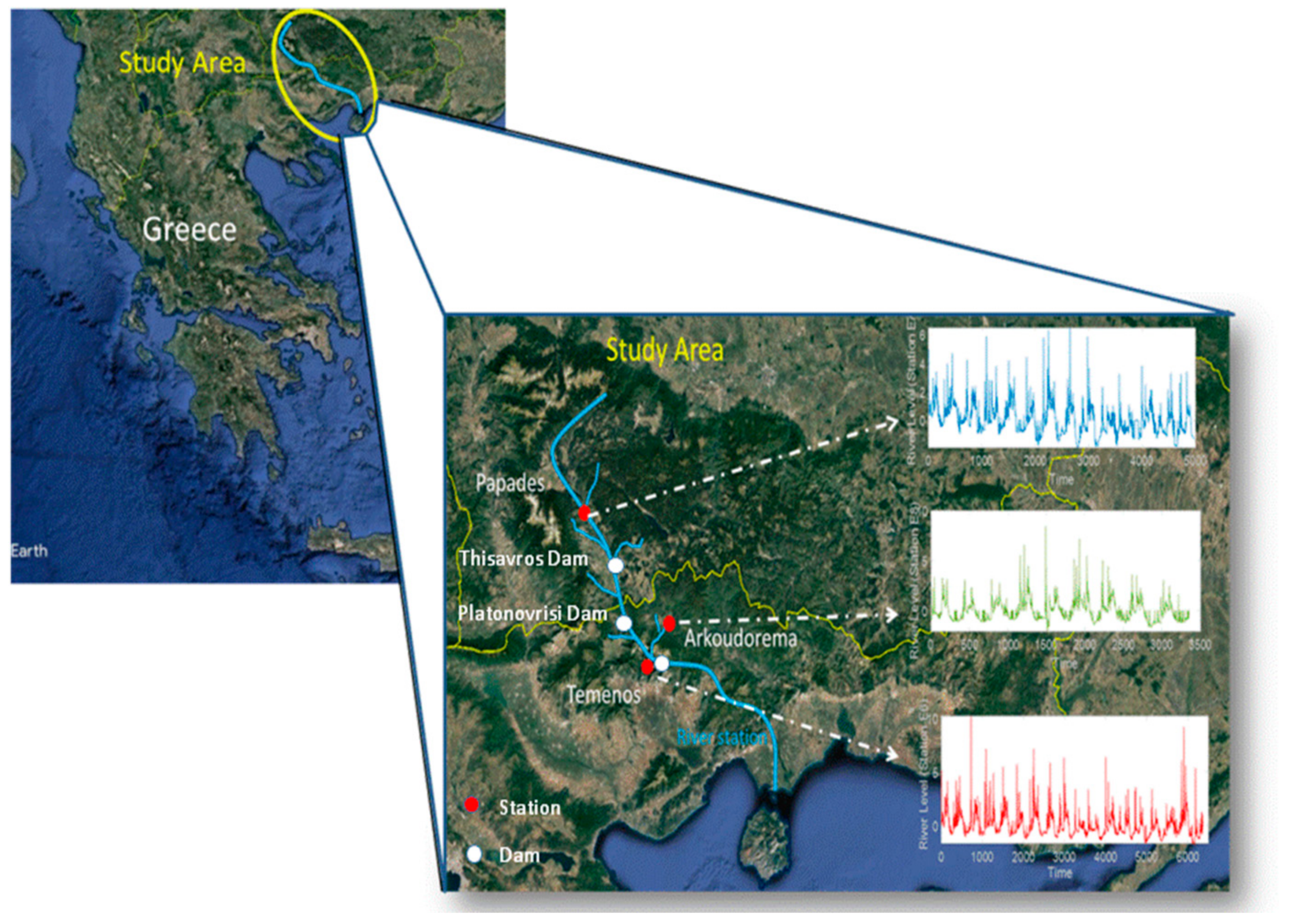
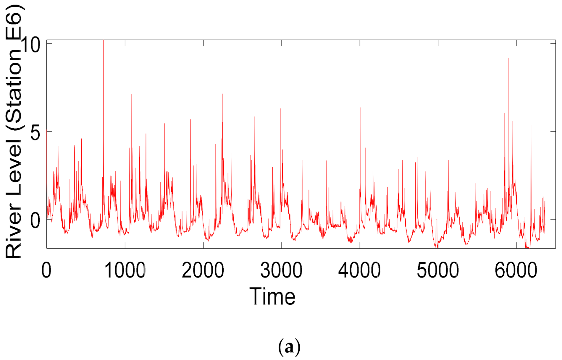
2. Area under Study—Data Description

Nestos is one of the largest rivers in the Balkan Peninsula, with a total length of 243 km. It originates in Bulgaria (113 km) and continues flowing in Greece (130 km), in the regions between Macedonia and Thrace. Nestos flows into the Thracian Sea, containing a network of 25 affluents (Arkoudorema, Diavolorema, Kousdorema, etc.) [35]. The physical location is depicted in Figure 1.

The Nestos River has a Mediterranean ecosystem, where the summer is warm and dry and winter is mild and rainy. The climate of the mountainous region of the river is characterized by a harsh winter and hot summer, with August and September being the driest months [36].

The area of our interest is the river’s flow from Papades (Northern Greek border with Bulgaria) to Temenos and Arkoudorema (river’s mountain region), where the hydrometric stations are located and the data were extracted (Greek Electric Company (DEH) (Figure 1). The daily data come from three measurement stations: (a) Temenos station measurements cover the longest time period from 1 January 1980 to 3 June 1997, (b) Papades station measurements cover the time period from 1 January 1980 to 17 August 1993 and (c) Arkoudorema station measurements cover the shortest time period, from 1 November 1992 to 4 January 2002 (

Table 1. The three stations from which observations were taken, the time period of data and the number of observations.

Station Name	Period of Data	Number of Observations
Temenos (E6)	1 January 1980–3 June 1997	6364
Papades (E7)	1 January 1980–17 August 1993	4978
Arkoudorema (E8)	1 November 1992–4 January 2002	3352

).

There are many tributaries and streams that collect water in the ground of the prefecture and flow into Nestos. It should be noted that the Papades (E7) measuring station and Temenos (E6) station are situated in the main part of the river, while the Arkoudorema (E8) station is located in a tributary that flows into the main river. Moreover, three major dams (those of Temenos, Platanovrisi and Thisavros) have been constructed in a row. The construction lasted almost 10 years (Platanovrisi Dam: 1989–1999, Thisavros Dam: 1986–1996). All three are hydroelectric, while the dam of Temenos is simultaneously an accumulator for irrigation purposes and that of Platanovrisi is simultaneously a warehouse. Nowadays, two of them are operated, those of Thisavros and Platanovrisi, and have been created upstream the two corresponding lakes. As the Papades station is above the points where the dams have been constructed, the measurements are not affected. In addition, the Arkoudorema station is outside the influence of the dams. The only direct influence of the dams on the measurement process has been at the Temenos station since 1986.

3. Methodology

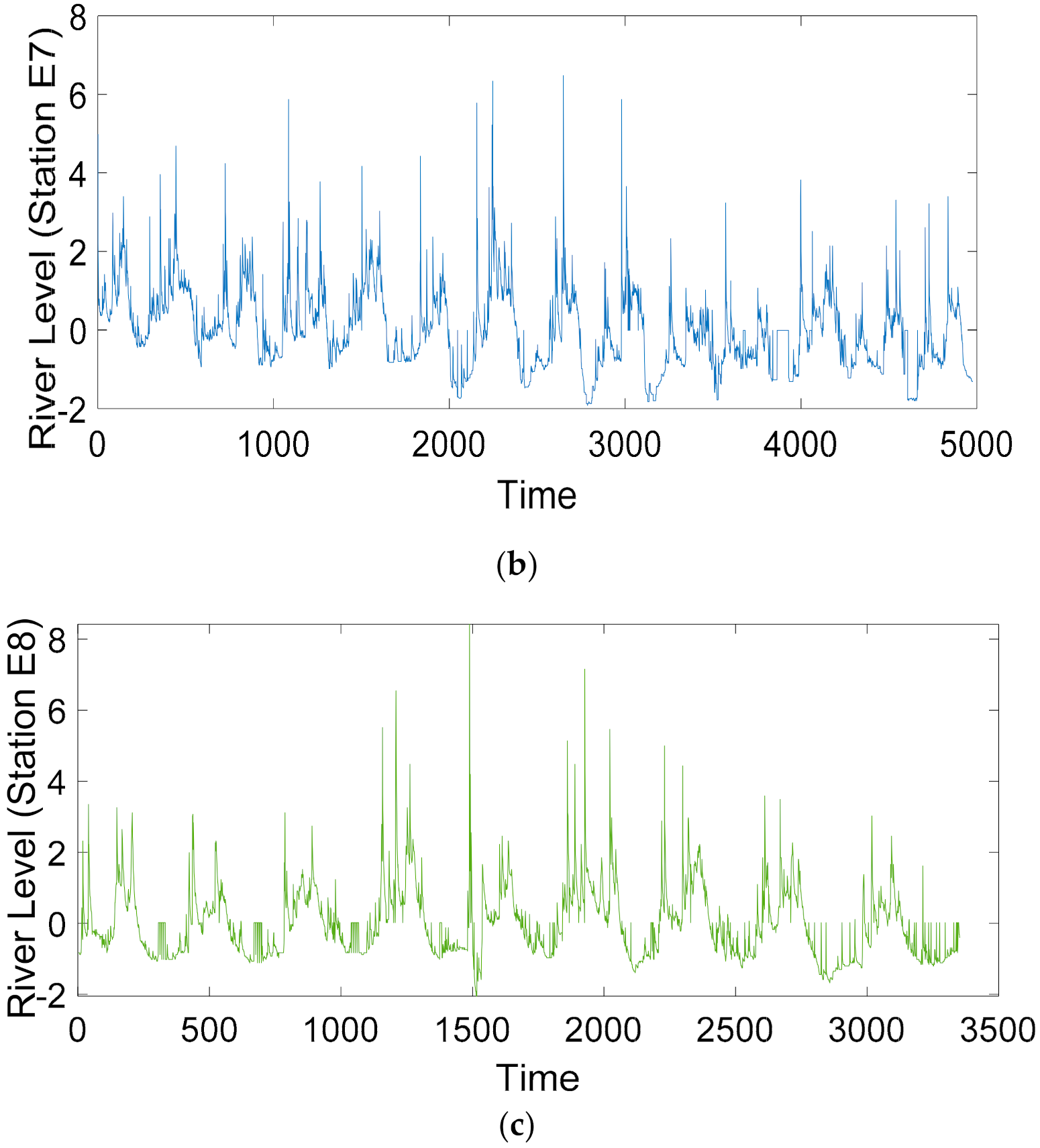
3.1. Recurrence Plots

A Recurrence Plot is a graphical tool introduced in 1987 by Eckmann et al. [37] in order to extract qualitative information on a dynamical system through study of its time series. One of its advantages is that it can be applied on non-stationary data. The first step in order to construct a Recurrence Plot is to make a phase space reconstruction from the time series. For the phase space reconstruction, we first estimate the time lag for the embedding. Fraser and Swinney [38] suggested the Average Mutual Information Equation (1) in order to choose the appropriate time lag, with the main advantage being compared with the autocorrelation function, as it takes into account non-linear correlations.

$$I=-{\sum }_{ij}^N{p}_{ij}\left(t\right)ln\frac{p_{ij}\left(t\right)}{p_i\left(t\right)p_j\left(t\right)}$$

(1)

where $p_i\left(t\right)$ is the probability in the i-interval to exist a value of the time series and $p_{ij}\left(t\right)$ is the joint probability if, in the i-th interval, there exists an observation; then, in the j-th interval, there exists an observation at a later time τ. Fraser and Swinney [38] report that if, at a point τ, the average mutual information falls to its first minimum value, then this time lag is a reasonable choice for the proper time delay for the estimation of the embedding dimension. Taking this lag into account, False Nearest Neighbors is a method with which one can estimate the optimal embedding dimension m by observing false neighbors in the phase space [39].

In the next step, we embed the time series, forming a sequence of vectors ${\overrightarrow{x}}_i=[x\left(t_i-\left(m-1\right){\tau }_d\right), x\left(t_i-\left(m-2\right){\tau }_d),\dots ,x\left(t_i\right)\right]$(${\tau }_d$ is the estimated time lag), and then we calculate the distances $d_{i,j}=\Vert {\overrightarrow{x}}_i-{\overrightarrow{x}}_j\Vert$ between points $i,j$ in the m-dimensional reconstructed phase space. A matrix of distances called a recurrence matrix is constructed then according to Equation (2)

$$R_{i,j}=\mathsf{\Theta }\left({\epsilon }_{\iota }-\Vert {\overrightarrow{x}}_i-{\overrightarrow{x}}_j\Vert \right),x_i\in R^m,i,j=1,2,\dots .,N$$

(2)

where $R_{i,j}$ is the recurrence matrix, m is the embedding dimension, ε the cutoff distance for the points considered to be recurrent and $\mathsf{\Theta }$ is the Heaviside function. The Heaviside function takes a value equal to 1 when the points are located at smaller distances than the cut-off distance ε; otherwise, $\mathsf{\Theta }$ = 0 (points are located at greater distances than the cut-off distance ε). On the texture of a Recurrence Plot, a black dot is placed at coordinates $\left(i,j\right)$ if $R_{i,j}=1$ and a white dot if $R_{i,j}=0$. Recurrence Plots are symmetric with respect to the main diagonal ($R_{i,i}=1$). When computing an RP, a norm must be chosen. In the present study, the Euclidean norm was used.

The main objective of an RP is to extract areas corresponding to the behavior of the dynamic system. The resulting patterns of the RP can provide information about the behavior of the data. Generally, an RP is a symmetrical matrix graph that represents those times at which the dynamic system recurs to a “state’’. The columns and rows correspond then to a certain pair of times. Specifically, the RP structure mainly contains lines parallel to the main diagonal (sign of deterministic processes), white regions (abrupt changes in the system’s dynamics) and isolated points (strong fluctuations) [13]. Recurrence Plots of deterministic processes may contain large diagonal lines, in contrast to Recurrence Plots of strongly fluctuating processes, which contain single isolated points. If, during the evolution of the system, there are states that are trapped in time, then vertical and horizontal lines appear on the RP’s texture, forming black regions.

3.2. Recurrence Quantification Analysis

In order to quantify the visual information of the RPs, Zbilut and Webber [12] and Marwan [13] introduced a number of quantities, giving rise to the so-called Recurrence Quantification Analysis (RQA). RQA provides an interesting framework for classification and characteristic time extraction since they are non-linear methods and take into account non-linearities in the system behavior. These quantifiers count the black dots on the Recurrence Plot and quantify the lines forming those dots (diagonal and vertical). We present briefly some of the RQA indices that have been proposed and we use for the present work:

• %Recurrence: The Recurrence Rate (RR) is the ratio of the number of recurrence points to the total number of points of the plot.

$$RR=\frac{1}{N^2}{\sum }_{i,j=1}^N{R}_{i,j} R_{i,j}=\left\{\begin{array}{c}1, \left(i,j\right) recurrent\\ 0, otherwise\end{array}\right.$$

(3)

2.

Average Diagonal Line Length: The average length of the diagonal line segments in the plot, excluding the main diagonal.

$$L=\frac{{\sum }_{l=l_{min}}^{N}lP\left(l\right)}{{\sum }_{l=l_{min}}^{N}P\left(l\right)}$$

(4)

3.

Trapping Time, TT: This shows the average length of the vertical lines. The Trapping Time represents the average time that the system has been trapped in the same state.

$$TT=\frac{{\sum }_{\upsilon ={\upsilon }_{min}}^N\upsilon P^{\epsilon }\left(\upsilon \right)}{{\sum }_{\upsilon ={\upsilon }_{min}}^N{P}^{\epsilon }\left(\upsilon \right)}$$

(5)

We calculated the Recurrence Rate, Trapping Time and Averaged Diagonal Length, as these measures are directly connected with the dynamic evolution of the river water level. They give us information from which we can export results on the existence of typical characteristic times of river water level changes. Different values correspond to different regimes. A high value is indicative of an underlying deterministic mechanism with few perturbations, while a lower value indicates that a perturbative mechanism is also present. As far as TT is concerned, it is used since it indicates how long the system is located (“trapped”) around a given system state. A small value indicates that the system spends a small amount of time in a given state, while a larger one is indicative that the system stays for longer time in a given state (condition).

The Recurrence Plot and the Recurrence Quantification Measures were created using the tool “Command Line Recurrence Plots” [40] and CRP toolbox version 5.12 [41], which is available online: https://tocsy.pik-potsdam.de/crp.php (accessed on 10 December 2021). For estimating time lag τ and embedding dimension m, we used the toolbox “Time Series Analysis” (TI.SE.AN.) [42].

For further understanding, we applied the Recurrence Quantification Analysis with epoqs in order to locate the time periods in which the changes took place. Epoqs are equidistant time periods that are calculated along the main diagonal of the Recurrence Plot and help us to locate possible phase transitions during the evolution of the system [15]. According to the method, transitions of the system are located by the visualization of the Recurrence Plots’ structure and delimiting regions with different textures (diagonal lines, white areas or isolated points). Dissimilarities in structure between the located regions, along with the Recurrence Quantification Analysis, are a good indication of transitions between the states of the system under study.

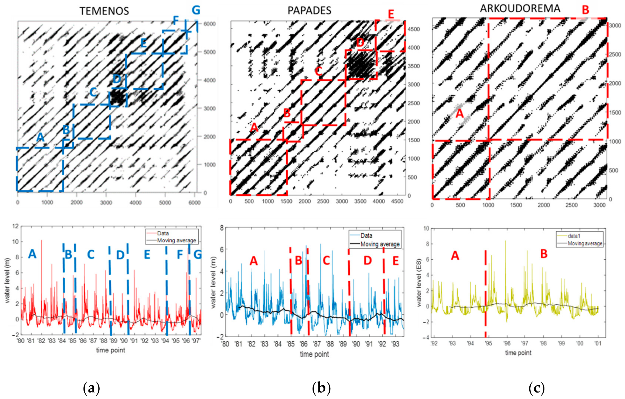
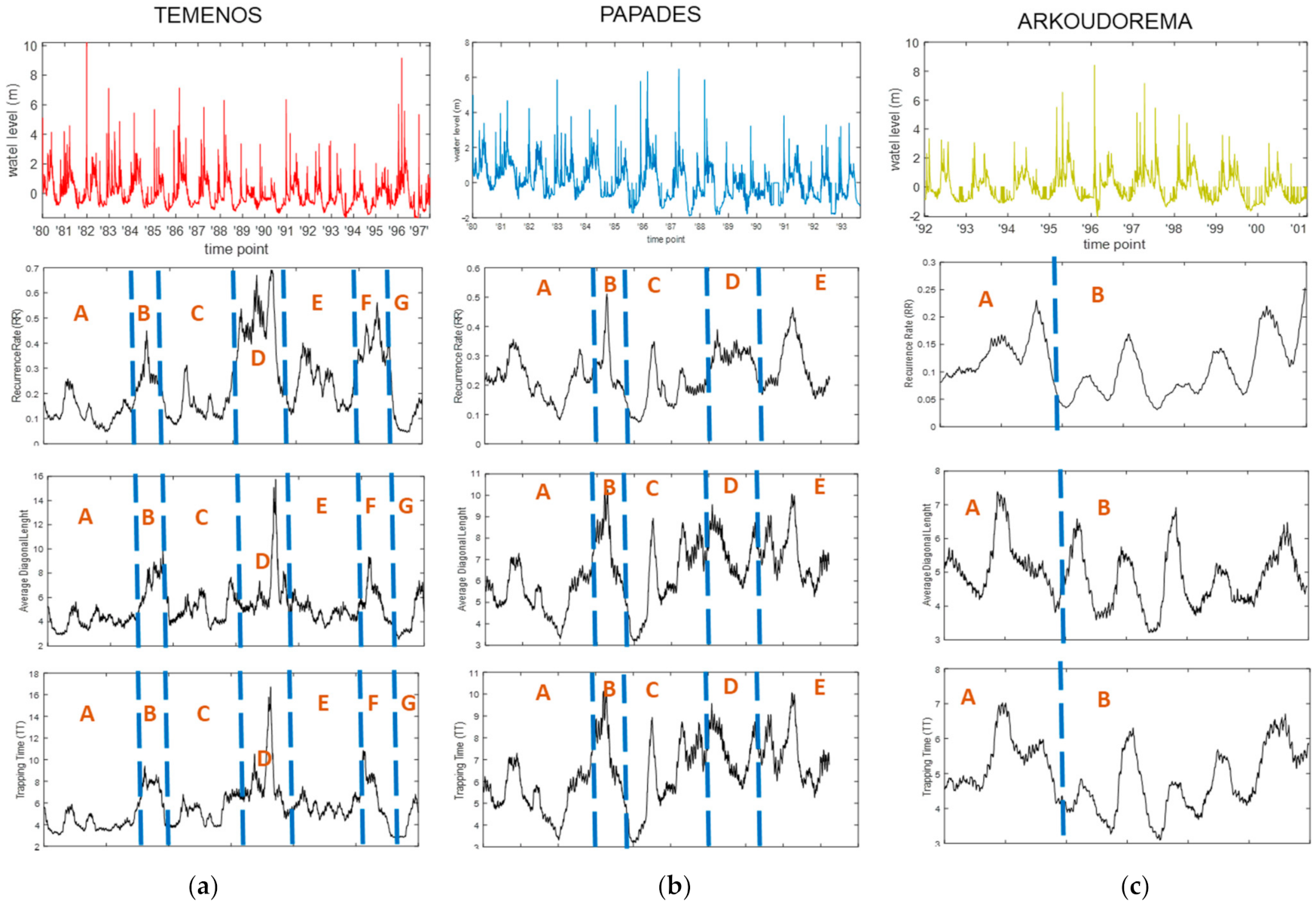
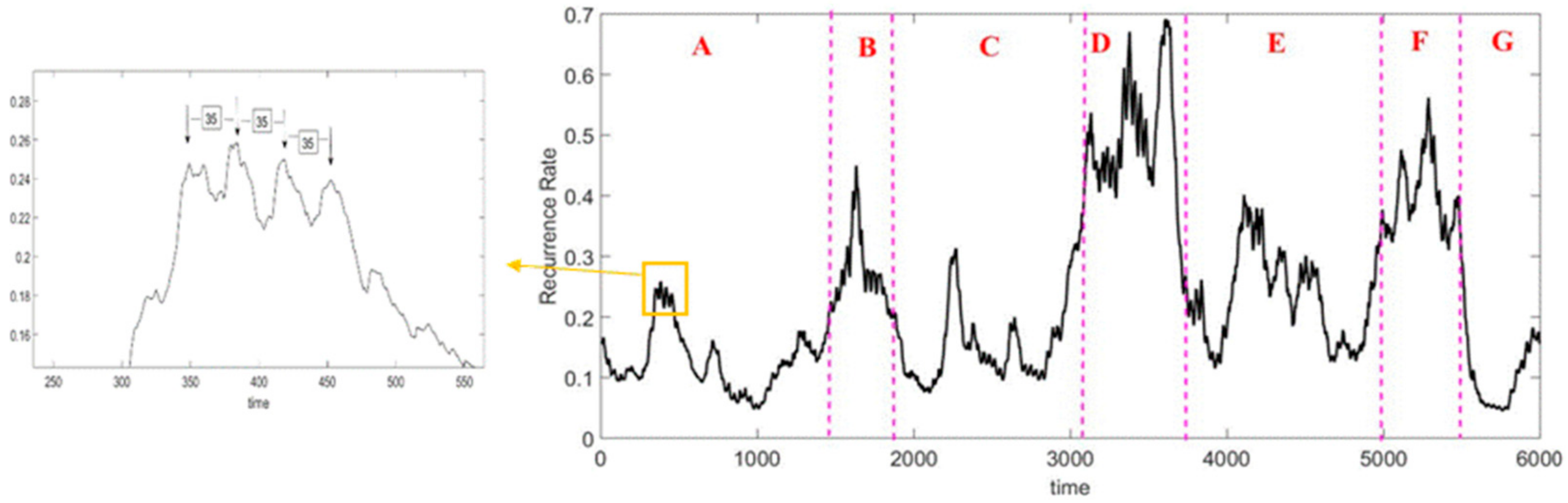
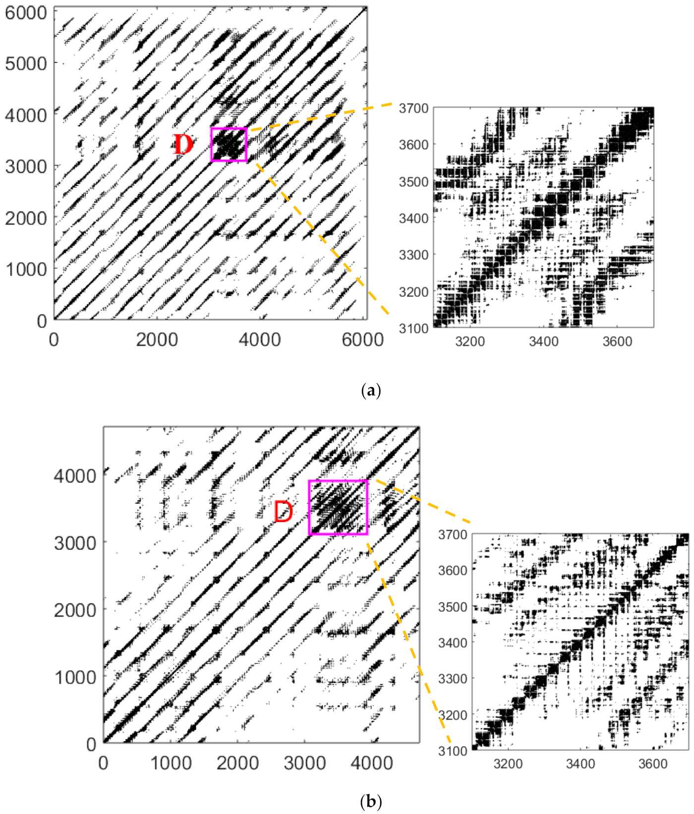
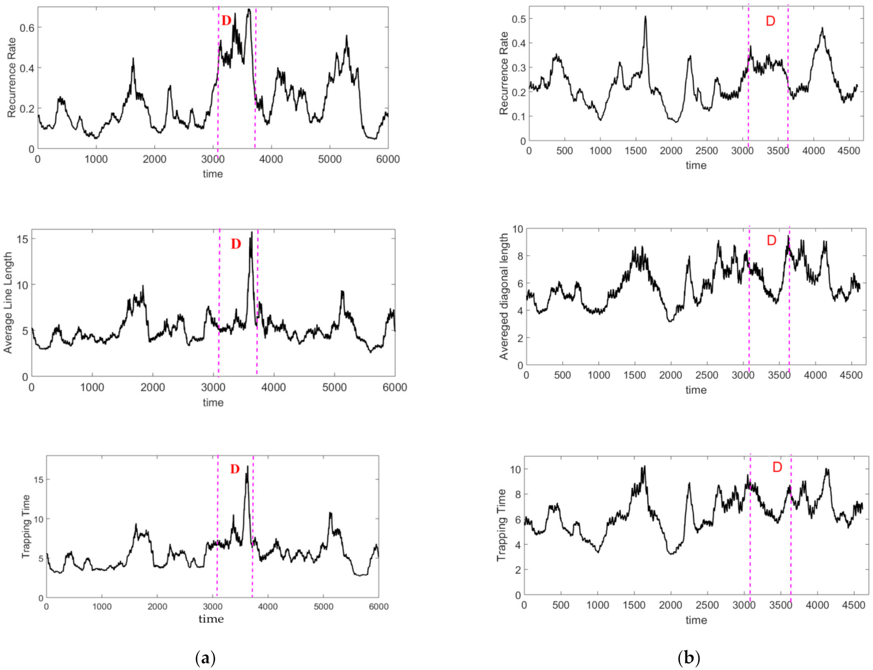
4. Results and Discussion

The Recurrence Plots were constructed by using the proper embedding parameters after the normalization of the time series to zero mean and a standard deviation of one (i.e., the new normalized time series is given by $Y=\frac{X-\overline{X}}{\sigma })$ (Figure 2). For the Recurrence Plot analysis, we proceeded to the estimation of time delay, τ (Average Mutual Information) and the embedding dimension m (False Nearest Neighbor) [39], and the residuals method was used on each time series to eliminate trends from the time series (

Table 2. The embedding parameters and the threshold ε of each of the three stations.

Station Name	Embedding Dimension, m	Time Delay, τ	Τhreshold, ε
Temenos	9	35	1.5
Papades	9	33	1.8
Arkoudorema	9	28	1.6

). For the proper estimation of the embedding, the criterion of below 10% falseness of nearest neighbors was used [39], and for the time delay, the criterion of the first minimum of the Average Mutual Information was used [38] (Table 2).

The Recurrence Plots’ parameters, embedding dimension, time delay and threshold [43] of each normalized time series constructed are presented in Table 2. For the Recurrence Plot threshold ε, the optimum rate of recurrences is the value of 0.02; thus, the Recurrence Rate parameter was calibrated to almost 2% [12]. Moreover, threshold estimation fulfills the topological criterion [40]. The thresholds are given in Table 2.

We note that the Recurrence Plots method is able to provide accurate results even if applied on time series with trends [13].

Figure 3a–c present the time series along with the corresponding RPs for the Temenos, Padades and Arkoudorema stations, respectively. From a global inspection of the RPs of each station, we can clearly see large diagonal segments forming lines parallel to the main diagonal. Generally, the distances between the main diagonal lines of the RP shape give us information about the periodicity of the data we are studying. Specifically, the distance between these segments is 365 points, which is consistent with the physical interpretation of the data (annual periodicity of the data).

In addition, in Figure 4a, where the Temenos area is presented, one can clearly see the extracted time series that correspond to the first recorded year (1980). In this figure, one can see that, during the first months, the river level rises to a peak at the end of April. Then, during summer, it gradually decreases (at the end of August) and then again rises during autumn.

As is known, each parallel line in the main diagonal appears when the time series shows periodicity; we observe that, in all three cases, there are parallel lines that characterize the periodicity of the system. In particular, these temporal changes through time series appear in the graph of the Temenos station, where there are 16 diagonal parallel lines, in that of Papades (11 parallel lines) and in the case of Arkoudorema (8 parallel lines).

From Figure 3, we find that there are similarities and differences in the RPs, where black and white denser and thinner areas are observed in each graph, particularly along the main diagonal number of squared regions observed. These regions contain either diagonal structures forming lines or dense structures with diagonal and vertical lines. Some regions contain white areas. These regions can give useful information about the dynamics of the system in time (phase transitions).

Consequently, in Figure 4a–c, we present the corresponding RP graphs, where the characteristic areas have been noted. In addition, in the time series, the results of the moving average analysis are depicted.

First, in all cases, in the RPs, we sketched the areas where they are clearly visible. Next, these separated regions were marked in the time series profile, where we also illustrated the curve of moving average analysis.

In particular, in the Temenos RP, we can distinguish different areas: A, B, C, D, E, F. Regions A, C, E have almost the same representation and contain large diagonal structures with small diagonal lines on each structure, separated with small white areas (recurrent states in short characteristic times), while region D is denser than the other. Each of these areas corresponds to regions almost with the same water level profile. Furthermore, in time series figure, we have marked the characteristic region.

In the Papades RP, we can also separate five regions (A, B, C, D, E) according to the representation of the RP. While areas A, C and E have almost the same representation, regions B and E have a denser structure. Finally, in the Arkoudorema RP, two areas can be distinguished (A and B). In general, through an in-depth inspection of the RP, we can select times at which transitions or other interesting events occur and identify characteristic patterns.

The small region B on the Temenos and Papades stations’ Recurrence Plots contains a white region and a dense region with parallel and diagonal lines, revealing a process trapped in time after an abrupt change in dynamics. Parallel lines to the main diagonal are characteristic of region F on the Temenos Recurrence Plot, indicating determinism with recurrent states in long characteristic times. Region D on the Recurrence Plot referring to the Temenos station contains denser structures with diagonal and vertical lines and isolated points, revealing non-deterministic processes, similar to region D on the Recurrence Plot referring to the Papades station.

Region G on the Recurrence Plot referring to Temenos station, as well as region B on the Recurrence Plot referring to the Papades station, contain white bands, revealing abrupt changes in the system dynamics.

The Recurrence Plot referring to the Arkoudorema station presents different textures, with two different regions, where region A contains large diagonal structures with small diagonal lines on each structure, separated with small white areas (recurrent states in short characteristic times), and region B contains white bands and small diagonal lines, revealing abrupt changes in the dynamics of the system. One can see that the statistics of the moving average, in all three cases, cannot distinguish the characteristic areas, providing no significant contribution of pure statistical measures in the study of non-linear dynamics.

Recurrence Plots seem to be informative, but, since the above regional estimations were made by visualization of the RPs, we proceeded to specify the locations of these regions by constructing epoqs and quantifying the RPs’ structures using Recurrence Quantification Analysis (RQA). RQA allows the quantification of the complex structure of the Recurrence Plots, and measures the recurrence point density and the diagonal and vertical line structures of the RP. These features are able to identify and quantify transitions between different system states and permit us to identify patterns in the system behavior.

Finding System Transitions by Constructing Sliding Windows (Epoqs)

As already mentioned, the aim of our study was to locate system transitions, so we proceeded to Recurrence Quantification Analysis constructing epoqs. We constructed sliding windows (epoqs) that covered a 1 year time evolution of the system (environmental systems such as Nestos River depend on seasonal and monthly changes). In order to locate phase transitions with more accuracy during the evolution of the system, we set the windows to overlap over 1 day each. In this way, 5999 epoqs for the Temenos station, 4613 epoqs for the Papades station and 2987 epoqs for the Arkoudorema station were constructed, and, on each window (epoq), Recurrence Quantification Analysis parameters were computed.

Figure 5 presents the results of the performance of Recurrence Rate, Average Line Length and Trapping Time for Temenos station (Figure 6 column A), Papades station (Figure 6 column B) and Arkoudorema station (Figure 6 column C). These three parameters are very important for the procedure of detecting transitions in system dynamics because they depend on the rate of points forming diagonal lines (Average Line Length), on the rate of points forming vertical lines (Trapping Time) and the total number of points of a Recurrence Plot (Recurrence Rate). They also depict the behavior of the system over time.

Considering the Recurrence Plots’ structures and the above analysis of the visualization of the RP (Figure 4), we proceeded to the observation of the RQA diagrams of all stations’ parameters (Figure 6, Figure 7 and Figure 8). Variations in the values of the RQA parameters could show differences between system states and locate any possible phase transition. It is of great importance to locate the variations between values of the Recurrence Rate parameter. In the Recurrence Plot’s texture, white regions do not contain points, resulting in small values of the Recurrence Rate parameter. On the other hand, black regions contain points, either isolated or points forming lines, resulting in large Recurrence Rate values. In addition to Recurrence Rate variations, values of the Average Line Length and Trapping Time parameters further assist in distinguishing isolated points from points forming lines [12].

Thus, according to variations in the Recurrence Rate parameter (either large or small values) and the values of parameters counting recurrent points forming lines (Average Line Length and Trapping Time), we can separate regions for the Temenos, Papades and Arkoudorema stations, locating system transitions (

Table 3. Regions at each station after the location of transition points.

Station Name	Regions
Temenos	A (1–1450)	E (3701–5000)
	B (1451–1800)	F (5001–5500)
	C (1801–3100)	G (5501–5999)
	D (3101–3700)
Papades	A (1–1450)	D (3101–3700)
	B (1451–1800)	E (3701–4607)
	C (1801–3100)
Arkoudorema	A (1–910)	B (911–2987)

).

It should be noted that these conclusions cannot be led by the time series profile. To obtain a better insight into the dynamics, we discuss the Recurrence Quantification Analysis with epoqs on the parameters of Recurrence Rate, Average Line Length and Trapping Time. By examining the Recurrence Rate parameter of Temenos station (Figure 6), first, we observe small peaks, where, if we zoom out, we can see that we have an average distance between peaks corresponding to 35 days. This time interval corresponds to almost a month and it is equal to the time delay estimated from the Average Mutual Information.

As observed on the Recurrence Rate, Average Line length and Trapping Time diagrams at regions A, C, E of Temenos station, regions A, C of Papades station and region A of Arkoudorema station, there are relatively small values of these three parameters. Specifically, along these regions, most values of the Temenos Recurrence Rate parameter are low, with the exception of region E, where the RR values fluctuate strongly. Along these regions, the Average Line Length and Trapping Time values are below 0.5, quantifying recurrent states in short characteristic times, providing the river level variation but in a typical way as the seasons change during these time periods (river level is low during dry months and high during rainy months).

Different behavior of the level of the river is apparent when we observe large values of the Recurrence Rate together with small values of the Average Line Length and Trapping Time parameters (<0.5) at region D of Temenos and Papades stations, a sign of non-deterministic processes, meaning that, during these times, dry periods may last for a shorter period of time than usual (water level not stable at low values for a short time) or rainy periods may last for a shorter period than usual (water level does not stay stable at high values for long time).

A different non-deterministic behavior is shown in region B of Arkoudorema station, where the three parameters change abruptly, meaning that the level of the river fluctuates strongly.

Finally, we observe that the values of the three parameters change at region B of the Temenos and Papades stations, with large values after an abrupt changes in low-valued parameters in region A. In this case, the weather conditions cause the level of the river to become trapped in time. During this time, dry periods may last longer (water level stays almost stable at low values) or rainy periods may last longer (water level stays almost stable at high values)

As can be seen from the results, the Arkoudorema station displays different behavior from the other two stations. Arkoudorema is an affluent of the Nestos River and one of the largest water contributors [34].

With a more focused observation of the Recurrence Plots’ patterns for different stations, one can see regions that provide similar structures. The most characteristic is region D of the Temenos and Papades Recurrence Plots, whose structure is dense. A large number of recurrent points are located in these regions, with the texture forming diagonal and vertical lines. However, many isolated points can be observed.

The above observations analyzed and quantified in the previous section with the RQA method focused initially on the values of the Recurrence Rate in region D combined with the values of the Average Line length and Trapping Time parameters. Thus we observe large values of the Recurrence Rate, contrary to the small values of the Average Line Length and Trapping Time parameters. This indicates the non-deterministic behavior of the system during this period (Figure 8), as analyzed in the different stations. This becomes a more interesting result since, during these periods (1986–1989), the construction of the Platanovrisi and Thisavros Dams started, with a strong impact on the dynamics of the river. It is obvious that the dynamics of the Nestos River at both stations (Papades, Temenos) were affected since the level of the river changed its behavior abruptly, without natural causes.

5. Conclusions

During the present study, the non-linear methods of Recurrence Plots and Recurrence Quantification Analysis with epoqs were employed to analyze daily time series of the water level of the Nestos River, with RQA parameters locating transitions of the system. Parameters such as Recurrence Rate and Average Line Length in combination with Trapping Time were used in order to extract useful information about the dynamics of the system, as with the case of trends and monthly and annual variations. We show that the proposed methodology provides useful information that can characterize different time periods (region at RPs) throughout the dynamic evolution, which could provide a better understanding of the river water level system complexity.

In addition, we show that non-linear methods such as RPs and RQA can be used in addition to statistics, providing more accurate results regarding the dynamic evolution of the system.

Overall, the employed analysis reveals the dynamic transitions of the Nestos River and its affluents, including Arkoudorema, and is exploitable for energy policy investors to successfully evaluate the optimal river flow performance in order to construct dams for energy production, which will benefit the local economy and society under the rules for the protection of the environment. The analysis could be extended to other river basins and also to a range of years in order to obtain more accurate conclusions.

Moreover, an important extension of this study would be to incorporate the methodology of Recurrence Plots and Recurrence Quantification Analysis into the field of Earth system dynamics and climate science [44].

References

1. Booij, M.J. Impact of climate change on river flooding assessed with different spatial model resolutions. J. Hydrol. 2005, 303, 176–198. [Google Scholar] [CrossRef]
2. Li, Z.; Xu, Z.; Shao, Q.; Yang, J. Parameter estimation and uncertainty analysis of SWAT model in upper reaches of the Heihe river basin. Hydrol. Process. 2009, 23, 2744–2753. [Google Scholar] [CrossRef]
3. Garba, H.; Ismail, A.; Batagarawa, R.L.; Ahmed, S.; Ibrahim, A.; Bayang, F. Climate Change Impact on Sub-Surface Hydrology of Kaduna River Catchment. Open J. Mod. Hydrol. 2013, 3, 115. [Google Scholar] [CrossRef] [Green Version]
4. Ye, L.; Zhou, J.; Zeng, X.; Tayyab, M. Hydrological Mann-Kendal Multivariate Trends Analysis in the Upper Yangtze River Basin. J. Geosci. Environ. Prot. 2015, 3, 34. [Google Scholar] [CrossRef]
5. Diaz-Nieto, J.; Wilby, R.L. A comparison of statistical downscaling and climate change factor methods: Impacts on low flows in the River Thames, United Kingdom. Clim. Change 2005, 69, 245–268. [Google Scholar] [CrossRef]
6. Kasamba, C.; Ndomba, P.M.; Kucel, S.B.; Uamusse, M.M. Analysis of Flow Estimation Methods for Small Hydropower Schemes in Bua River. Energy Power Eng. 2015, 7, 55–62. [Google Scholar] [CrossRef] [Green Version]
7. Georgakakos, A.P.; Marks, D.H. A new method for the real-time operation of reservoir systems. Water Resour. Res. 1987, 23, 1376–1390. [Google Scholar] [CrossRef]
8. Movahed, M.S.; Hermanis, E. Fractal analysis of river flow fluctuations. Phys. A Stat. Mech. Appl. 2008, 387, 915–932. [Google Scholar] [CrossRef] [Green Version]
9. Kędra, M.; Wiejaczka, L.; Wesoły, K. The Role of Reservoirs in Shaping the Dominant Cyclicity and Energy of Mountain River Flows. River Res. Appl. 2015, 32, 561–571. [Google Scholar] [CrossRef]
10. Kantz, H.; Schreiber, T. Nonlinear Time Series Analysis, 2nd ed.; Cambridge University Press: Cambridge, UK, 2003. [Google Scholar]
11. Porporato, A.; Ridolfi, L. Nonlinear analysis of river flow time sequences. Water Resour. Res. 1997, 33, 1353–1367. [Google Scholar] [CrossRef]
12. Zbilut, J.P.; Webber, C.L., Jr. Embeddings and delays as derived from quantification of recurrence plots. Phys. Lett. A 1992, 171, 192–203. [Google Scholar] [CrossRef]
13. Marwan, N. Encounters with Neighbors. Ph.D. Thesis, University of Potsdam, Potsdam, Germany, 2003. [Google Scholar]
14. Marwan, N.; Carmenromano, M.; Thiel, M.; Kurths, J. Recurrence plots for the analysis of complex systems. Phys. Rep. 2007, 438, 237–329. [Google Scholar] [CrossRef]
15. Wendi, D.; Merz, B.; Marwan, N. Assessing Hydrograph Similarity and Rare Runoff Dynamics by Cross Recurrence Plots. Water Resour. Res. 2019, 55, 4704–4726. [Google Scholar] [CrossRef]
16. Wendi, D.; Merz, B.; Marwan, N. Novel Quantification Method for Hydrograph Similarity. In Advances in Hydroinformatics; Springer: Singapore, 2020; pp. 727–734. [Google Scholar] [CrossRef]
17. Facchini, A.; Mocenni, C.; Marwan, N.; Vicino, A.; Tiezzi, E. Nonlinear time series analysis of dissolved oxygen in the Orbetello Lagoon (Italy). Ecol. Model. 2007, 203, 339–348. [Google Scholar] [CrossRef]
18. Keegan, A.P.; Zbilut, J.P.; Merritt, S.L.; Mercer, P.J. Use of recurrence plots in the analysis of pupil diameter dynamics in narcoleptics. Chaos Biol. Med. 1993, 2036, 206–215. [Google Scholar] [CrossRef]
19. Mestivier, D.; Chau, N.P.; Chanudet, X.; Bauduceau, B.; Larroque, P. Relationship between diabetic autonomic dysfunction and heart rate variability assessed by recurrence plot. Am. J. Physiol. Circ. Physiol. 1997, 272, H1094. [Google Scholar] [CrossRef]
20. Karakasidis, T.E.; Liakopoulos, A.; Fragkou, A.; Papanicolaou, P. Recurrence Quantification Analysis of Temperature Fluctuations in A Horizontal Round Heated Turbulent Jet. Int. J. Bifurc. Chaos 2009, 19, 2487–2498. [Google Scholar] [CrossRef]
21. Aceves-Fernandez, M.A.; Ramos-Arreguín, J.M.; Pedraza-Ortega, J.C.; Sotomayor-Olmedo, A.; Tovar-Arriaga, S. Finding Trends of Airborne Harmful Pollutants by Using Recurrence Quantification Analysis. Am. J. Environ. Eng. 2011, 1, 10–14. [Google Scholar] [CrossRef] [Green Version]
22. Builes-Jaramillo, A.; Marwan, N.; Poveda, G.; Kurths, J. Nonlinear interactions between the Amazon River basin and the Tropical North Atlantic at interannual timescales. Clim. Dyn. 2018, 50, 2951–2969. [Google Scholar] [CrossRef]
23. Semeraro, T.; Luvisi, A.; Lillo, A.O.; Aretano, R.; Buccolieri, R.; Marwan, N. Recurrence Analysis of Vegetation Indices for Highlighting the Ecosystem Response to Drought Events: An Application to the Amazon Forest. Remote Sens. 2020, 12, 907. [Google Scholar] [CrossRef] [Green Version]
24. Mohammed, A.M. Analysis and predictive validity of Kelantan River flow using RQA and Time Series Analysis. Kuwait J. Sci. 2021, 48. [Google Scholar]
25. Panagoulia, D.; Vlahogianni, E.I. Recurrence quantification analysis of extremes of maximum and minimum temperature patterns for different climate scenarios in the Mesochora catchment in Central-Western Greece. Atmos. Res. 2018, 205, 33–47. [Google Scholar] [CrossRef]
26. Trauth, M.H.; Asrat, A.; Duesing, W.; Foerster, V.; Kraemer, K.H.; Marwan, N.; Maslin, M.; Schaebitz, F. Classifying past climate change in the Chew Bahir basin, southern Ethiopia, using recurrence quantification analysis. Clim. Dyn. 2019, 53, 2557–2572. [Google Scholar] [CrossRef] [Green Version]
27. Zhao, Z.Q.; Li, S.C.; Gao, J.B.; Wang, Y.L. Identifying Spatial Patterns and Dynamics of Climate Change Using Recurrence Quantification Analysis: A Case Study of Qinghai–Tibet Plateau. Int. J. Bifurc. Chaos 2011, 21, 1127–1139. [Google Scholar] [CrossRef]
28. Acharya, U.R.; Faust, O.; Kadri, N.A.; Suri, J.S.; Yu, W. Automated identification of normal and diabetes heart rate signals using nonlinear measures. Comput. Biol. Med. 2013, 43, 1523–1529. [Google Scholar] [CrossRef] [PubMed]
29. Addo, P.M.; Billio, M.; Guégan, D. Nonlinear dynamics and recurrence plots for detecting financial crisis. N. Am. J. Econ. Financ. 2013, 26, 416–435. [Google Scholar] [CrossRef] [Green Version]
30. Karain, W.I. Detecting transitions in protein dynamics using a recurrence quantification analysis based bootstrap method. BMC Bioinform. 2017, 18, 525. [Google Scholar] [CrossRef] [Green Version]
31. Valavanis, D.; Spanoudaki, D.; Gkili, C.; Sazou, D. Using recurrence plots for the analysis of the nonlinear dynamical response of iron passivation-corrosion processes. Chaos 2018, 28, 085708. [Google Scholar] [CrossRef]
32. Fragkou, A.D.; Karakasidis, T.E.; Nathanail, E. Detection of traffic incidents using nonlinear time series analysis. Chaos 2018, 28, 063108. [Google Scholar] [CrossRef]
33. Charakopoulos, A.; Karakasidis, T.; Sarris, L. Pattern identification for wind power forecasting via complex network and recurrence plot time series analysis. Energy Policy 2019, 133, 110934. [Google Scholar] [CrossRef]
34. Fernandez-Fraga, S.M.; Aceves-Fernandez, M.A.; Rodríguez-Resendíz, J.; Pedraza-Ortega, J.C.; Ramos-Arreguín, J.M. Steady-state visual evoked potential (SSEVP) from EEG signal modeling based upon recurrence plots. Evol. Syst. 2019, 10, 97–109. [Google Scholar] [CrossRef]
35. Diadovski, I.K.; Atanassova, M.P.; Ivanov, I.S. Integral assessment of climate impact on the transboundary Mesta River flow formation in Bulgaria. Environ. Monit. Assess. 2007, 127, 383–388. [Google Scholar] [CrossRef]
36. Sylaios, G.; Kamidis, N. Environmental impacts of large-scale hydropower projects and applied ecohydrology solutions for watershed restoration: The case of Nestos River, Northern Greece. In The Rivers of Greece; Springer: Berlin/Heidelberg, Germany, 2017; pp. 379–401. [Google Scholar]
37. Eckmann, J.-P.; Kamphorst, S.O.; Ruelle, D. Recurrence Plots of Dynamical Systems. Europhys. Lett. 1987, 4, 973–977. [Google Scholar] [CrossRef] [Green Version]
38. Fraser, A.; Swinney, H.L. Independent coordinates for strange attractors from mutual information. Phys. Rev. A 1986, 33, 1134. [Google Scholar] [CrossRef]
39. Kennel, M.B.; Brown, R.; Abarbanel, H.D.I. Determining embedding dimension for phase-space reconstruction using a geometrical construction. Phys. Rev. A 1992, 45, 3403. [Google Scholar] [CrossRef] [Green Version]
40. Marwan, N. Command line Recurrence Plots. 2006. Available online: http://tocsy.pik-potsdam.de/commandline-rp.php (accessed on 10 December 2021).
41. Marwan, N. Cross Recurrence Plot Toolbox, Reference Manual, Version 5.12, Release 25; Potsdam Institute for Climate Impact Research: Potsdam, Germany, 2008. [Google Scholar]
42. Hegger, R.; Kantz, H.; Schreiber, T. Nonlinear Time Series Analysis TISEAN Version 3.0.1. 2007. Available online: http://www.mpipks-dresden.mpg.de/~tisean/Tisean_3.0.1/index.html (accessed on 10 December 2021).
43. Andreadis, I.; Fragkou, A.D.; Karakasidis, T.E. On a topological criterion to select a recurrence threshold. Chaos 2020, 30, 013124. [Google Scholar] [CrossRef]
44. Boers, N.; Kurths, J.; Marwan, N. Complex systems approaches for Earth system data analysis. J. Phys. Complex. 2021, 2, 011001. [Google Scholar] [CrossRef]
Figure 1. Nestos River location in Balkan Peninsula and region under study, with the location of each hydrometric station (Papades, Temenos, Arkoudorema).
Appliedmath 02 00001 g001
Figure 2. Normalized time series of Nestos River water level for (a) Temenos, (b) Papades and (c) Arkoudorema station, respectively.
Appliedmath 02 00001 g002aAppliedmath 02 00001 g002b
Figure 3. Recurrence Plot and the corresponding time series of (a) Temenos (E6), (b) Papades (E7) and (c) Arkoudorema (E8) stations, respectively.
Appliedmath 02 00001 g003
Figure 4. The Recurrence Plots with regions and the corresponding time series of Nestos River water level: (a) Temenos, (b) Papades and (c) Arkoudorema station.
Appliedmath 02 00001 g004
Figure 5. The Recurrence Quantification Analysis parameters (Recurrence Rate, Averaged Diagonal Line Length and Trapping Time) of (a) Temenos, (b) Papades and (c) Arkoudorema stations, respectively.
Appliedmath 02 00001 g005
Figure 6. Recurrence Rate parameter of Temenos station.
Appliedmath 02 00001 g006
Figure 7. The Recurrence Plots of (a) Temenos and (b) Papades stations focused on region B (zoomed).
Appliedmath 02 00001 g007
Figure 8. Region D of Recurrence Quantification Analysis parameters of (a) Temenos and (b) Papades stations.
Appliedmath 02 00001 g008