Article

Random Forest Classifier Algorithm of Geographic Resources Analysis Support System Geographic Information System for Satellite Image Processing: Case Study of Bight of Sofala, Mozambique

Department of Geoinformatics, Faculty of Digital and Analytical Sciences, Universität Salzburg, Schillerstraße 30, A-5020 Salzburg, Austria
Coasts 2024, 4(1), 127-149; https://doi.org/10.3390/coasts4010008
Submission received: 25 December 2023 / Revised: 15 February 2024 / Accepted: 20 February 2024 / Published: 26 February 2024
(This article belongs to the Special Issue Measuring Shoreline Variability and Understanding It's Local Impacts)

Abstract

:
Mapping coastal regions is important for environmental assessment and for monitoring spatio-temporal changes. Although traditional cartographic methods using a geographic information system (GIS) are applicable in image classification, machine learning (ML) methods present more advantageous solutions for pattern-finding tasks such as the automated detection of landscape patches in heterogeneous landscapes. This study aimed to discriminate landscape patterns along the eastern coasts of Mozambique using the ML modules of a Geographic Resources Analysis Support System (GRASS) GIS. The random forest (RF) algorithm of the module ‘r.learn.train’ was used to map the coastal landscapes of the eastern shoreline of the Bight of Sofala, using remote sensing (RS) data at multiple temporal scales. The dataset included Landsat 8-9 OLI/TIRS imagery collected in the dry period during 2015, 2018, and 2023, which enabled the evaluation of temporal dynamics. The supervised classification of RS rasters was supported by the Scikit-Learn ML package of Python embedded in the GRASS GIS. The Bight of Sofala is characterized by diverse marine ecosystems dominated by swamp wetlands and mangrove forests located in the mixed saline–fresh waters along the eastern coast of Mozambique. This paper demonstrates the advantages of using ML for RS data classification in the environmental monitoring of coastal areas. The integration of Earth Observation data, processed using a decision tree classifier by ML methods and land cover characteristics enabled the detection of recent changes in the coastal ecosystem of Mozambique, East Africa.
PACS:
91.10.Da; 91.10.Jf; 91.10.Sp; 91.10.Xa; 96.25.Vt; 91.10.Fc; 95.40.+s; 95.75.Qr; 95.75.Rs; 42.68.Wt
MSC:
94A08; 68U10; 54H30; 86A30; 86-08; 86A99
JEL Classification:
Y91; Q20; Q24; Q23; Q3; Q01; R11; O44; O13; Q5; Q51; Q55; N57; C6; C61

1. Introduction

1.1. Background

Remote sensing (RS) data have long been an important and efficient source of information for environmental monitoring, being one of the main data sources for mapping and detecting patterns in biodiversity across large spatial areas [1]. The information from the Earth Observation satellite missions, which is provided quickly and effectively, has sufficient coverage, and the high quality of images has ensured numerous applications of RS data in modern geospatial studies and cartographic works [2]. Information derived from satellite images enables the identification of landscape characteristics that affect biodiversity patterns, the structural and functional properties of landscapes, and the spatial extent of different components of ecosystems. Such advantages of RS data enable using both high-resolution and medium-resolution products in vegetation and land cover mapping, in order to detect patterns in vegetation changes and to track ecological interactions through time series analyses [3,4,5].
Applications of RS data in environmental analyses include diverse types of satellite images, which can be used for the effective interpretation of Earth’s landscapes, including Sentinel 2 data [6,7,8], a National Oceanic and Atmospheric Administration Advanced Very High Resolution Radiometer [9,10], Satellite Pour l’Observation de la Terre (SPOT), [11], and Landsat [12,13,14,15,16], as well as combinations thereof [17,18]. For instance, the recent Global Land Cover 2000 map was based on an analysis of the vegetation sensor on board the SPOT-4 satellite, using methods of digital image processing and GIS [19,20]. Moreover, RS data can be integrated with information about the environmental setting for analysis, mapping, and modeling purposes. For instance, Landsat scenes widely used for landscape mapping include the data acquired from its various sensors, such as the Multispectral Scanner (MSS), Thematic Mapper (TM), Enhanced Thematic Mapper Plus (ETM+), and recent products of the Operational Land Imager and Thermal Infrared Sensor (OLI/TIRS), or used with data integration [21,22,23].
The Landsat OLI-TIRS satellite missions measured the surface reflectivity and scattering in the multi-spectral bands, which resulted in its successful application during recent decades [24]. Its capacity to discriminate between different vegetation types was demonstrated in previous investigations [25,26,27,28]. In cloud-prone and rainy areas typical of coastal regions of tropical African countries, however, the use of RS data is restricted by atmospheric effects, such as the attenuation of signals and cloud coverage during wet periods. Therefore, an analysis of vegetation should be based on cloud-free images or with minimized cloudiness (below 10%). Moreover, the remaining atmospheric effects should be minimized using advanced methods of computer vision. These include, for instance, atmospheric scattering or haze, which occur as a result of suspended dust that accumulates in relatively dry air. Such effects may lead to color distortion of the images and worsen image quality through impaired visibility, which may affect image analysis.
As a result, the processing of such data requires advanced methods of satellite image processing, e.g., removing noise, highlighting edges, and improving image contrast through the correction of atmospheric effects. This is possible using computer vision and machine learning (ML) algorithms for data processing and visualization due to their impressive computational and spatial analysis capabilities [29,30,31]. The most important advantage of ML techniques is that they are capable of automagically deriving information from existing datasets. Moreover, ML methods apply programming algorithms that enable them to excel in complex analyses and modeling of geospatial data [32]. In environmental studies, valuable insights from ML include information extraction from complex terrain and heterogeneous landscapes, such as coastal regions. Such features of ML facilitate environmental analysis and enhanced planning and management of the coastal zones.
Establishing new methods of Earth Observation data processing, such as with ML, requires the application of programming approaches that enable the automation of tasks [33,34]. Indeed, the integrated use of programming scripts, ML capabilities, and cartographic methods has provided powerful tools for RS data processing, with the aim of mapping, analyzing, and monitoring coastal areas using the distinctive sensor responses of land cover types. Thus, scripting and programming approaches enable overcoming the ambiguities in image classification resulting from similarities in the spectral reflectance of various land cover types, especially with medium-resolution Landsat data, maintaining the high-automation streams of modeling. Advancements in computer processing; ML methods; and the development of scripting languages, such as Python, used either alone or as integrated tools and add-ons in a geographic information system (GIS), have allowed for an advanced approach to cartography and image processing. Such methods support accurate satellite data processing and analysis, which have made dynamic vegetation modeling possible [35].

1.2. Related Works

Generally speaking, the accuracy of classification of the vegetation types in heterogeneous landscapes using satellite images mainly depends on the sensitivity of sensor backscattering to differences between the phenological characteristics of plant leaves. Alternatively, they should also be sensitive to the variations in structure of the other land cover types such as bare land or urban areas with dominating impervious surfaces. Hence, different interactions between the sensor backscatter and the structure of the canopy of landscape patches can provide novel information on ecological structure. Nevertheless, many recent studies [36,37,38,39,40] noted the evident advantages of using ML methods in image processing. For instance, Ref. [41] found that the use of deep learning (DL) modeling in remote sensing data processing could improve the accuracy of the classification.
Earlier studies have also reported that the classification precision was significantly improved when the computer vision algorithms of DL for image analysis and interpretation were applied [42,43,44]. Similar studies also validated the potential of the use of ML methods in cartographic applications of RS data processing for mapping various vegetation classes. Thus, these methods were used for evaluation of the optimal combination of geospatial data used for separating different land cover classes [45,46]. These and other results reported in previous studies also indicated that the use of Python improves the performance of the classification and attains the required automation and accuracy level in the process of image classification [47,48,49]. Nevertheless, improvements and flexibility are achieved in the Geographic Resources Analysis Support System (GRASS) GIS software, which presents a smart combination of the existing Python libraries with cartographic toolsets and a powerful image processing functionality.
Since the release of the first version of GRASS GIS in 1984 [50], this instrument has been constantly improved, which resulted in a recent updated version of software 8.3.1. Nowadays, GRASS GIS presents a powerful geospatial data processing engine with an integrated suite of the existing modules for raster and vector data processing. The advances in technical progress and the rapid development of cartographic instruments along with the improvements in programming algorithms resulted in various types of modules of GRASS GIS that include diverse geospatial data processing tools. The applications of such tools can be found in a variety of case studies. To mention a few of them, the use of GRASS GIS in geographic studies includes environmental monitoring [51,52], time series and massive data analysis [53,54], hydrological modeling [55], computing landscape diversity, image segmentation [56,57], and geomorphometric modeling [58]. These examples prove the effectiveness of the GRASS GIS for image processing and remote sensing data analysis.

1.3. Objectives and Motivation

The primary objective of the present research is to determine the spatio-temporal changes in the land cover types of coastal Mozambique through the application of machine learning methods to remote sensing data analyses. In view of the advantages of the ML methods briefly discussed above, this study applies such methods and presents the case of image processing using the GRASS GIS module r.learn.train for image classification. Specifically, the random forest (RF) algorithm of the ML method is employed in this study with the sample coastal area of eastern Mozambique, Bight of Sofala. Using ML algorithms embedded in the modules of GRASS GIS enables us to perform a supervised classification using training pixels of raster tiles and the integrated Python Scikit-Learn library [59] for modeling vegetation in coastal areas.
The goal of this study is to develop a workflow using several modules of GRASS GIS for ML-based random forest techniques of image classification. To this end, the multi-spectral Landsat 8–9 OLI/TIRS images are used for land cover mapping of the coastal region of eastern Mozambique that encompasses the Bight of Sofala and cover a time gap from 2015 to 2023. Since the area is located in a cloud-prone and rainy region affected by occasional floods, the data are selected during the ‘dry’ period from August to September using optimal atmospheric conditions. Additionally, the images are corrected to improve their quality. In total, three scenes are used for classification and ML-based processing.
The main aim of this study is to evaluate short-term temporal dynamics in the region of the Bight of Sofala using advanced methods of cartographic scripting using the ML modules of the GRASS GIS. The methodology includes the extraction of training data from raster images, supervised ML methods that use ensemble classification, the regression tree method using RF, and cross-validation tasks. Technically, this paper demonstrates the advantages of using ML algorithms for RS data classification, as well as advanced approaches of cartographic mapping for the environmental monitoring of coastal areas. High robustness, versatility, and applicability of the RF algorithm motivated its application for processing satellite images in the shoreline regions which are notable for highly vulnerable environmental parameters. Due to the sensitivity of RF to noise and outliers in the pixel matrix, its application to image processing is beneficial for reducing the overfitting by averaging multiple decision trees, as demonstrated in this study. As a result, the use of RF algorithm enabled us to reduce the data processing time and to increase the accuracy of the Landsat 8–9 OLI/TIRS imagery.

2. Study Area

This study is located in the coastal area of Mozambique, western part of the Indian Ocean. Specifically, it investigates the region of the Bight of Sofala, where the estuary of the Beira river enters the Mozambique Channel (Figure 1).
As one of the developing countries of Africa, Mozambique is notable for its rapid land cover changes related to the environmental effects and urbanization. As a result, landscape dynamics have recently become one of the major issues of the country, which is reported in many relevant studies [61,62,
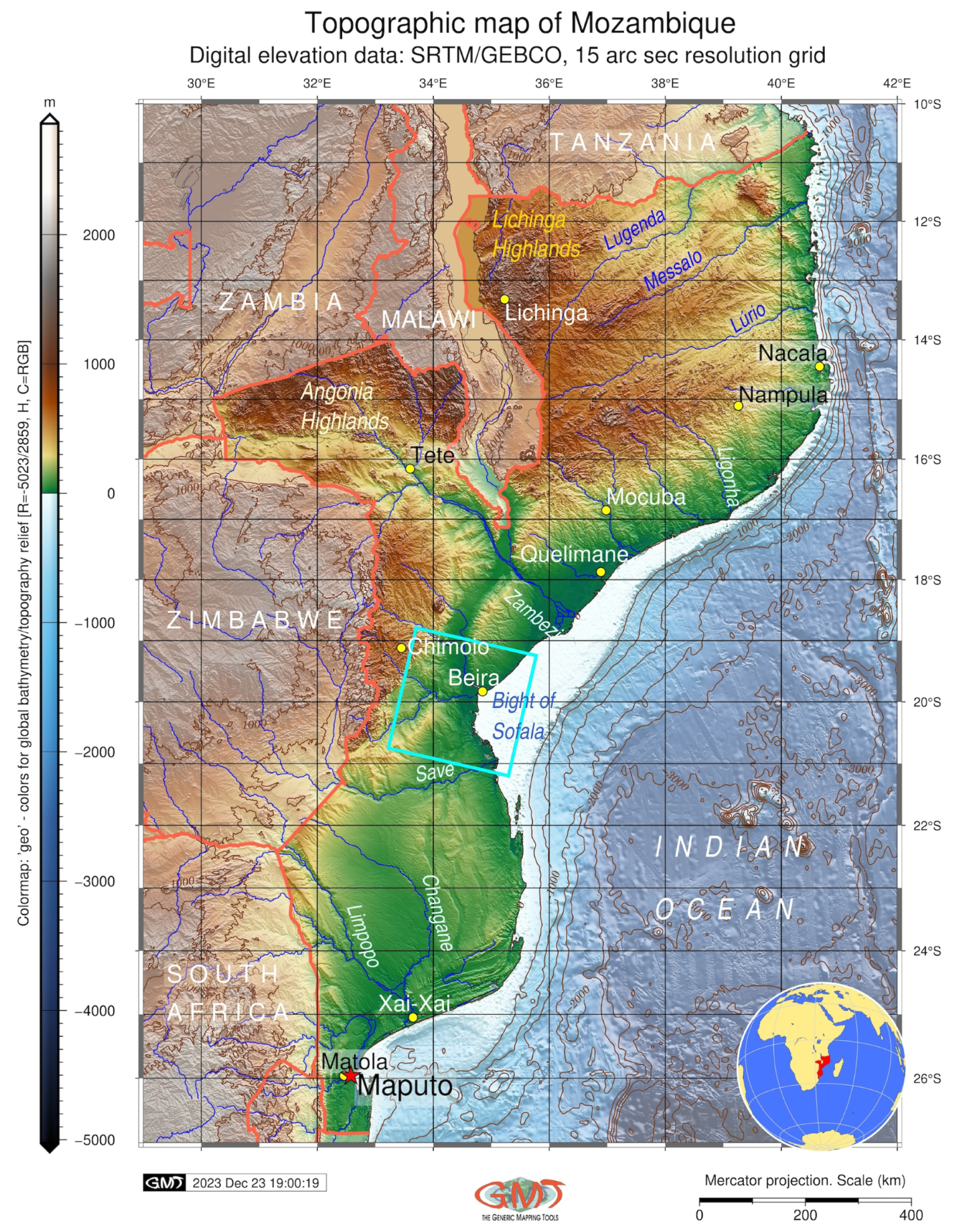
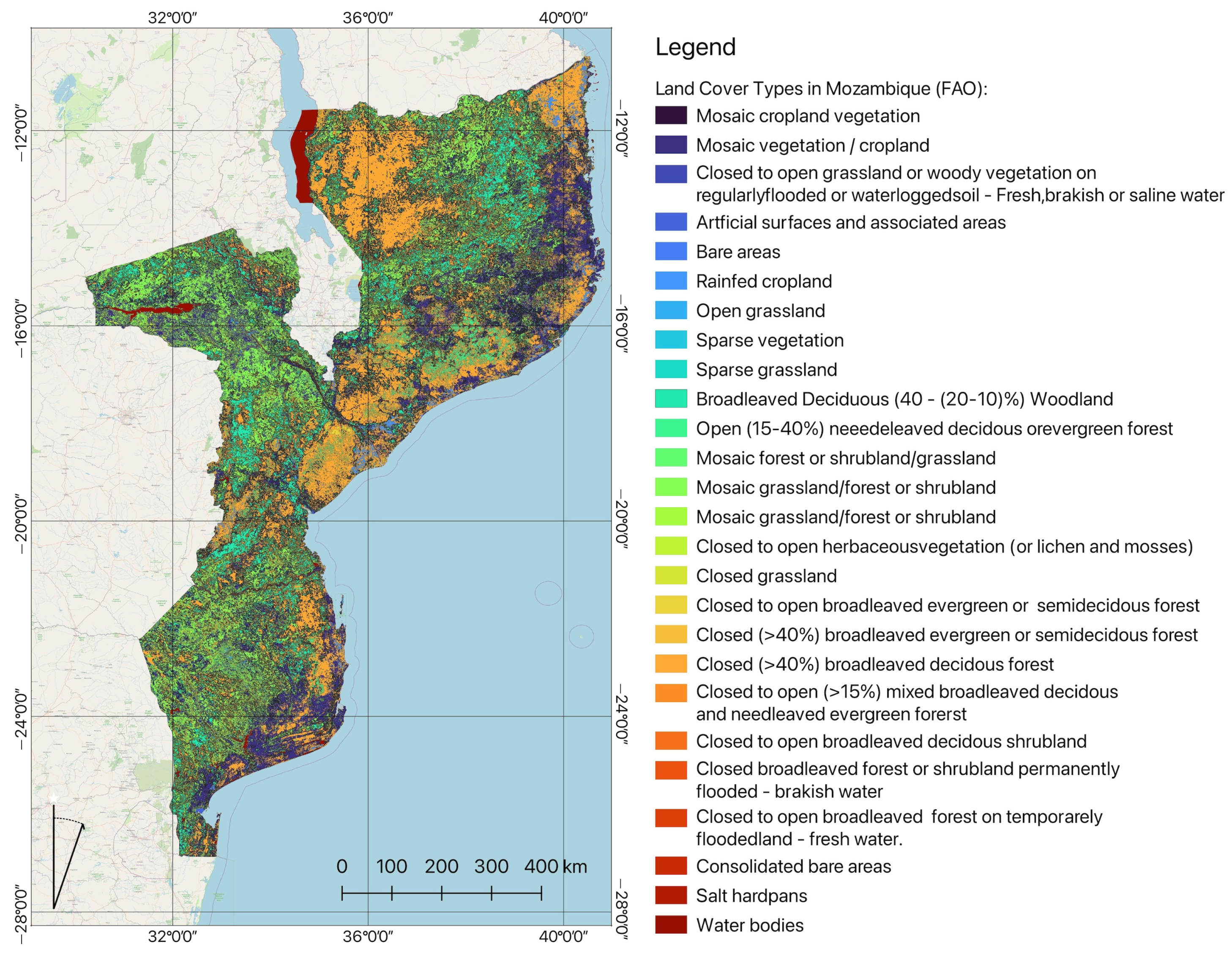
63]. Located on the southeast coast of Africa, Mozambique represents a country with diverse topographic forms and landscape setting. The most remarkable geomorphic features include a complex mix of the inland hills and low plateaus situated along the narrow coastal strip which contrast with rugged highlands located in the western parts of the country. Such variability in landscapes favors diversified vegetation structures, increases the biodiversity richness, and creates unique land cover patterns that are characteristic of Mozambique (Figure 2).
The major geomorphic types of Mozambique include numerous highlands interspersed with plateaus; covered with woodlands; and lowlands, which are situated mostly to the south of the Zambezi River—the major river of the country. The Zambezi River roughly separates the country into the northern and southern parts, which have notably distinct ecosystems. Being the fourth-longest river in Africa with a complex hydrological setting, it largely affects the distribution of plants and species in the surrounding landscapes and in the estuary zone, which is located to the north of the Bight of Sofala [64,65,66]. The hydrology of the Zambezi River is connected to the main channel and tributaries, and water management involves the eight countries surrounding the basin [67]. Thus, through the downstream and upstream movement of water that changes the local salinity and suspended sediments, the hydrology of Zambezi strongly influences the coastal ecosystems of the Sofala Bank [68]. Nevertheless, the recent construction of artificial dams has had significant environmental effects on the major floodplains. For instance, these include reduced water supply and river discharge [69] and increased sedimentation of the coastal landscapes of its estuary [70].
The coastal ecosystems in the Bight of Sofala are one of the most environmentally vulnerable regions in Mozambique. This is caused by multiple impacts from the climate setting and tidal hydrology [71] including tidal cycles, shelf circulation, and coastal currents [72]. In turn, the hydrological setting of the coastal ecosystems influence the patterns of primary production and the distribution of zooplankton, phytoplankton, and nutrients in the shelf waters [73]. Moreover, the rapid expansion of urban areas caused by population growth and economic pressure changes the landscapes. Such social processes result in urban sprawl, which changes the natural landscapes into artificial spaces [74]. Moreover, the Sofala Bank is known for its industrial shallow-water shrimp fishery [75,76,77], which creates additional pressure on the coastal ecosystems through the overexploitation of natural resources.
The repeated and severe floods and cyclones in western part of the Indian Ocean have a great influence on the landscapes and distribution of vegetation along the coasts of Mozambique. As a result, Mozambique is reported to be one of the most vulnerable south African countries to flooding and tropical cyclones. Such climatic hazards cause damage to the infrastructure and create additional factors to the disruption of ecosystems [78,79,80]. Another environmental issue in the coastal regions of Mozambique concerns the decline of mangroves, which is caused by the cumulative effects from anthropogenic activities and climate change [81]. At the same time, as highly productive coastal ecosystems with unique fauna and flora, mangrove swamps are important sources of natural resources and livelihoods for local people. Therefore, their decline and degradation negatively affect the sustainability of coastal ecosystems.
Over recent decades, the consequences of floods in Mozambique include the destruction of landscape structures [82] and crops during the flood period [83]. Moreover, this increased landscape fragmentation resulted in the continuous physical disintegration of habitats into smaller patches with decreased size and isolation between habitat clusters. The consequences of such processes negatively affect the biodiversity and species richness [84] as well as lead to disruptions in the coastal ecosystems [85]. In terms of social–economic aspects of Mozambique, climate-related natural hazards and disrupted landscapes affect the farming sector, fishery, and agriculture activities in the coastal areas of Mozambique.
All these factors are required for an effective environmental monitoring system. Specifically for the coastal regions of Mozambique, a data analysis enables us to define the cost of landscape restoration in the affected areas and to detect land cover changes. Proper land planning in the coastal areas of Mozambique requires the costly process of evaluating landscape dynamics, performing a climate change assessment, and carrying out an integrated socio-environmental analysis [86,87,88,89]. The lowest possible cost when monitoring the coastal areas of Mozambique can be achieved by evaluating the difference between land cover types and performing a patch analysis using the image classification and quantification of landscape fragments [90]. This is possible using cartographic mapping and a time series analysis of the satellite images [91,92,93]. Land surface topography, which varies significantly in Mozambique, influences the distribution of vegetation types that can be considered in agricultural planning, environmental management, and ecological monitoring of the coastal regions. For instance, to preserve the vulnerable ecosystem of the narrow strip along the coasts of the Bight of Sofala, operative monitoring using remote sensing data is a useful technical tool [94].

3. Materials and Methods

3.1. Workflow

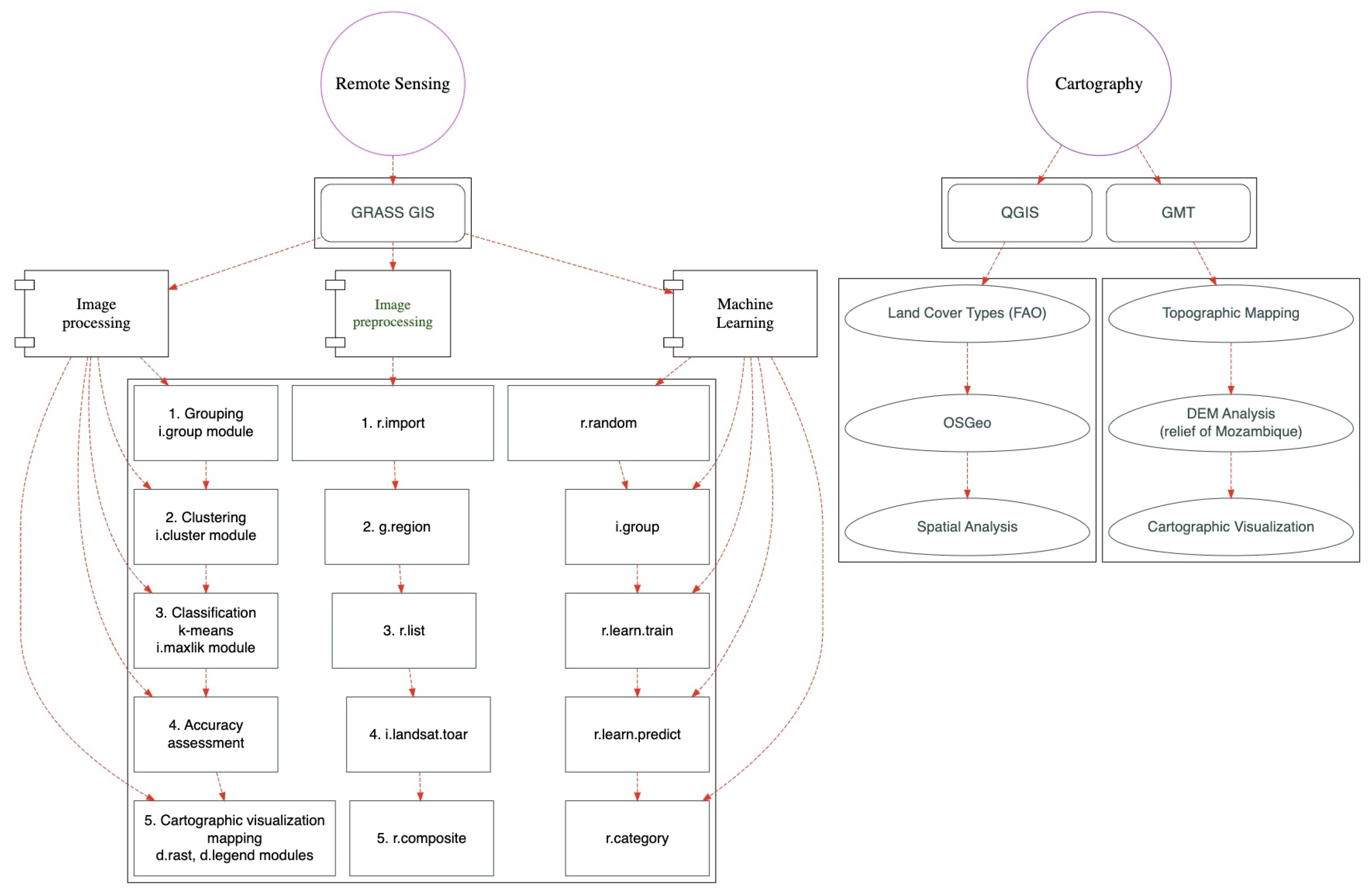
In this paper, multi-temporal Landsat 8–9 OLI/TIRS images were used for land cover mapping in the coastal region of the Bight of Sofala, eastern Mozambique, Indian Ocean. The methodology included the extraction of the training data from raster images, supervised ML using ensemble classification, the regression tree method using RF, and cross-validation tasks. A schematic view of the workflow in cartographic and remote sensing tasks is portrayed in Figure 3.
The workflow was completed using GRASS GIS software and includes the following 14 steps:
  • Image importation and interpretation using the Geospatial Data Abstraction Library (GDAL) and reprojection of images: Since all the images must be registered in the software and be coherent with each other, the registration procedure of the Landsat images was performed using the ‘r.import’ module. The metadata of the satellite images were set to the current region and checked to assess the suitability and quality control: data acquisition, cloudiness, sun elevation and geographic extent. Technically, this was carried out using the code “r.import input=/Users/<path>/ImageName.TIF output=ImageName extent=region resolution=region”. Here the path to the original image is provided in full; the resolution was set to the 30 m as for Landsat scenes.
  • Image preprocessing is a fundamental approach in remote sensing data analyses. It aims to prepare the images for further processing and analyses. Here, the Landsat images were integrated with GDAL and preprocessed using the ‘i.landsat.toar’ module, which calculates the top-of-atmosphere spectral reflectance and temperature for Landsat OLI/TIRS scenes. To this end, the information on sun elevation and the date of image acquisition were used from the metadata (product date). The digital numbers (DN) of the image pixels were converted to the top-of-atmosphere radiances (ToAR). The resulting output images were processed using the ‘i.landsat.toar’ module and the DN of the images were transformed, which calibrated the top-of-atmosphere reflectance.
  • To analyze the land cover types visible on the Earth’s surface as a representation landscape patches, color composites were created using bands of the satellite images. The image composites were generated using ‘r.composite’ for natural and false color composites using triplets of red, green, and blue bands merged into a single composite raster map by the following code (the example is for the band combination 7-5-3): “r.composite blue=L807 green=L805 red=L803 output=L8753 –overwrite”. Here, each band was selected for each of the RGB triplets (red, green, and blue), which enabled us to visualize the images in various combinations (natural and false color composites).
  • The landscapes of coastal Mozambique are characterized by a complex mosaic of heterogeneous land cover types that exhibit structural similarities in spectral reflectance. Therefore, a radiometric partition of the images was performed using the unsupervised k-means method with the ‘i.cluster’ module which employs computer vision techniques for objective and automatic recognition of land cover types. This method generates spectral signatures for different land cover types using a clustering algorithm that identifies the differences between various values of spectral reflectance for each pixels and assigns them to classes accordingly.
  • The generation of signature files for land cover types was performed using the ’signaturefile’ function of the ‘i.cluster’ module. The profiles of the spectral backscatter coefficient of the land cover types were generated and compared to the FAO classification with 10 major identified land cover classes in the coastal regions of Mozambique. Various characteristics of landscape patches were identified and compared for images taken at different periods as a time series.
  • Image classification was performed to identify land cover classes using the maximum likelihood method (‘i.maxlike’ module). This method was selected due to its versatility and ability to produce fast and accurate results. In essence, the MaxLike classification algorithm uses clusters generated in the previous step and classifies pixels in an iterative self-organizing process of image partition to produce a set of spectral classes. Afterwards, labels are assigned to the clusters automatically and maps are generated using a defined color palette.
  • The generation of training pixels from an older land cover classification using the ‘r.random’ module was performed to generate a set of raster point maps. This module creates a raster map which contains coordinates of points whose locations have been randomly determined to ensure the objectivity and randomness of the representative set of pixels. It includes randomly located cells and pixel points using a non-deterministic random seed. Technically, it was implemented by the following code: “r.random input=L8CL seed=100 npoints=1000 raster=L8CLroi”.
  • The creation of an imagery group with all Landsat OLI/TIRS multispectral bands that have 30 m resolution, excluding panchromatic bands: this was performed using ‘i.group’ module with the following code: “i.group group=L82015 input=L801,<...>,L807”.
  • A random forest classification model was trained using the ‘r.learn.train’ approach of the ML modules of the GRASS GIS. Practically, it was implemented using the following code: r.learn.train group=L82015 training_map=L82015roi.
    model_name=RandomForestClassifier n_estimators=500 save_model=rf_model.gz
  • Performing predictions using the ‘r.learn.predict’ module of GRASS GIS: This is an essential part of the ML data processing that uses a fitted Scikit-Learn estimator derived from Python to raster layers in a group of images. The implementation was performed using the code “r.learn.predict group=L8_2015 load_model=rf_model.gz output=rf_classification –overwrite”. The algorithm uses the training dataset generated in a previous step and applies the created model “rf_model.gz”. The main goal is to apply a fitted estimator from the Python’s ML library Scikit-Learn to the imagery group which was generated during the step “i.group”.
  • Checking raster categories using the module ‘r.category’: The category values and labels are displayed for the raster layer requested for the generated images. This is carried out by the command “r.category rf_classification”, which reports the data in the console output. In this case, 10 major land cover classes of the coastal area of Mozambique were identified by the computer vision, which were automatically applied to the classification results.
  • Visualization of the results was performed using the GRASS GIS module ‘r.colors’, which copies the color scheme from the land class training map to the output maps. For instance, the code for the maps of random forest classification was as follows: “r.colors rf_classification color=plasma-e”.
  • The results were mapped using a set of modules—‘d.rast’, ‘d.legend’, and ‘d.mon’—that represent the cartographic tools of GRASS GIS for mapping and the visual display of data. The files were then saved using the module ‘d.out.file’ as bitmap graphics. For instance, data visualization included the following snippets of code: “d.rast rf_classification d.legend raster=rf_classification title=“Random Forest: 2018” title_fontsize=14 font=“Helvetica” fontsize=12 bgcolor=white border_color=white”.
  • Interpretation of the results was based on the comparison of maps of land cover types of the Bight of Sofala, Eastern Mozambique, for 2015, 2018, and 2023 to analyze the spatio-temporal dynamics of land cover types in the coastal landscapes.

3.2. Data

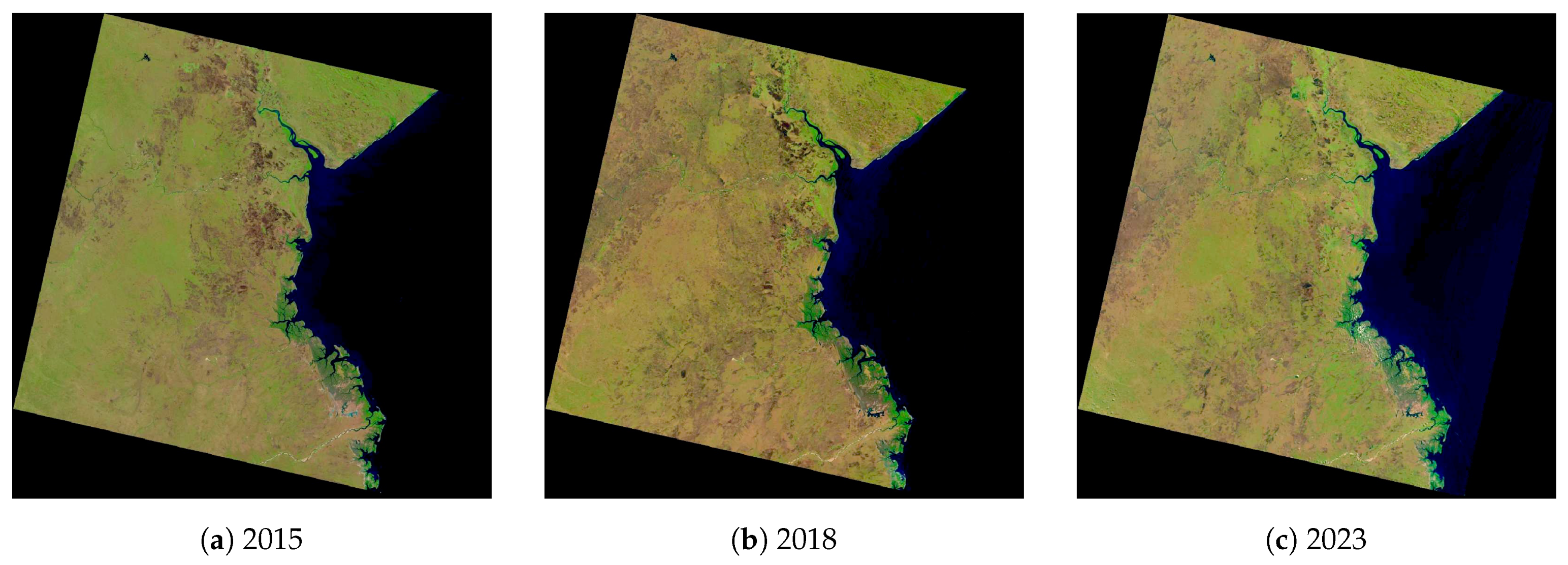
In this study, three multi-temporal images of the Landsat Operational Land Imager and Thermal Infrared Sensor (OLI/TIRS) were selected to produce a classification using machine learning. The images were chosen due to the high quality of the data, availability of the high-quality ’leaf-on’ data on coastal Mozambique, and coverage of the study area. The most essential technical characteristics of the images are summarized in Table 1.
The images are presented in Figure 4. Low cloudiness and acceptable resolution depend on the acquisition techniques of Landsat ensured by the United States Geological Survey (USGS).
The values of the cloud coverage were 0.01, 0.11, and 0.69 for the images from 2015, 2018, and 2023, respectively. The original satellite images are stored in Universal Transverse Mercator (UTM) Zone 36 for Mozambique. The terrain data of the study area used for topographic visualization are based on the General Bathymetric Chart of the Oceans (GEBCO) grid with high spatial resolution and accuracy (15 arc seconds) and visualized as the digital terrain model Shuttle Radar Topography Mission (SRTM). The topographic names are added according to the gazetteer of Digital Chart of the World (DCW).

3.3. Software

Traditional image processing methods rely on the use of GIS [95,96,97]. However, such methods have some drawbacks in that the human-controlled maintenance of workflow is required for image processing, classification, and analysis, which might be hard in case of image series. In contrast, script-based image processing uses the automation of data processing to derive information from the RS data [98]. An alternative approach is presented by machine learning (ML), which can be used as a descriptor of pixel values and partial replacement of the traditional methods using programming [99,100]. The ML is based on the algorithms of artificial intelligence, which include computer vision and statistical analyses. This study applies ML using the latest available version of GRASS GIS 8.3.1.
The installation of the program was performed using the ‘sudo port install grass’ with compilations, which includes the dependencies of the essential Python’s libraries and ML packages. The programming is implemented in the GRASS GIS as scripts. This automates the repeated steps of image processing to improve the workflow [101,102]. The data processing was performed on the MacBook Apple Sonoma (arm64 architecture). The Cooperative Computing Tools (CCTools), which enable large-scale distributed computations from clusters, were updated and installed using the sudo command as follows: ‘sudo port clean cctools’ and ‘sudo port -v install cctools’. After the CCTools and XCode were installed and activated, all the necessary updates in the libSystem of MacPorts were performed including the deactivated library libunwind-headers: ‘sudo port -f deactivate libunwind-headers’.
To employ the enhanced properties and improved functionality of GRASS GIS adjusted for satellite image processing, the Python-based modules and the toolchain GNU Compiler Collection (GCC) were used. The GCC 13 was installed accordingly for code compilation, supporting library dependencies through linking and conversion of GRASS GIS scripts into the binary executable format for assembly into executable files. The wxPython was installed additionally using the ‘sudo port install py311-wxpython-4.0’ command called from the MacPorts. The topographic map of the study area was made using the Generic Mapping Tools (GMT) software developed by [60], which represents a toolbox for geospatial data processing. The method used for mapping includes scripts that were derived from earlier works [103,104,105].

3.4. Scripting

The advanced script-based cartographic ML methods of the GRASS GIS for monitoring and mapping land cover types were built due to the growing demand for time- and cost-effective approaches in the cartographic workflow and remote sensing data analyses. It enables users to save time and resources while processing the geospatial datasets and to use open-source satellite images. Three major script-based toolsets were used in this study for the geospatial data analysis and environmental monitoring of West Africa:
  • GRASS GIS module ‘r.import’ was used for importing the data, Listing 1;
  • GRASS GIS module ‘r.composite’ was used for creating false and natural color composites, Listing 2;
  • GRASS GIS modules of ‘i.cluster’ and ‘i.maxlik’ were used for unsupervised image classification and accuracy assessment by computed rejection probability classes for classified pixels, Listing 3;
  • A combination of GRASS GIS modules ‘d.rast’, ‘d.legend’, ‘r.colors’, ‘d.mon’, ‘g.region’, and ‘d.out.file’ was used for mapping the output images, Listing 4;
  • GRASS GIS module ‘r.learn.train’ was used for random forest classification of machine learning (ML)-based supervised image classification using the training data generated in a previous step, Listing 5.
The main idea of this framework is to perform in a single workflow both image processing and mapping using scripts run from the console. This enables a user to reveal the technical performance of the automated geospatial data processing using a programming approach with three different programming suits of the script-based software. Such an approach demonstrated that the inclusion of scripts speeds up cartographic plotting and image processing and facilitates the research methodology. As mentioned earlier [106], the main advantage of scripts consists in automation of the process and repeatability of the workflow, which saves time. Using the information received from the automated image analysis and interpretation, we were able to detect the changes in the analysis of the landscapes of eastern Mozambique for evaluation of the environmental effects from climate change. This was achieved through a time series analysis of the satellite images taken for different years (2015–2023).
First, the GRASS GIS was started from the console, and then, the bands of the Landsat-8 OLIimage on 2015 were imported stepwise using the ‘r.import’ module, as shown in the script of Listing 1. The same algorithm was repeated for the Landsat images for 2018 and 2023.
Listing 1. GRASS GIS code for importing satellite images.
Coasts 04 00008 i001
Second, the color composites were created using Listing 2 for false and natural color composites with the case of an image from 2015. While true color composites show a representation of the Earth visible naturally to human eyes, false color composites better display selected features on the Earth (e.g., discrimination between water and land surfaces). This is done through a combination of visible red, green, and blue bands that correspond to the multispectral channels of the images.
Listing 2. GRASS GIS code for creating color composites.
Coasts 04 00008 i002
Third, the next step included clustering the image using the ‘i.cluster’ module. The computational region was set to the band of the Landsat image to match the scenes of the satellite images. The bands of the Landsat channels were grouped using the ‘i.group’ module, which is designed for grouping the data. The selected bands were used as grouped data during the clustering process. The signature file was generated using the ’signaturefile’ command. The image was classified into the 10 major classes of the classification scheme using the information from FAO. The unsupervised automated classification was performed using the ‘i.maxlik’ module. The complete script of this process is shown in Listing 3.
Listing 3. GRASS GIS code for grouping bands and clustering.
Coasts 04 00008 i003
Mapping and visualization of the output data was performed using a combination of the GRASS GIS modules ‘d.rast’, ‘d.legend’, ‘r.colors’, ‘d.mon’, ‘g.region’, and ‘d.out.file’, as shown for the Landsat image 2023 for a map produced using the classification and accuracy assessment with rejection probability classes (Listing 4). The same procedure was repeated for images taken in 2018 and 2023, respectively.
Listing 4. GRASS GIS code for data display, visualization and mapping.
Coasts 04 00008 i004
The accuracy assessment for the unsupervised classification was performed using the ’reject’ function of the ‘i.maxlik’ modules of GRASS GIS, which calculates the output raster map holding the reject threshold results. The aim of this step is to evaluate the confidence level at which each cell in the raster image is categorized during the classification process. The algorithm generates the reject threshold map layer, which contains the index to a computed confidence level for each classified pixel in the satellite scene. The predefined confidence intervals include sixteen values. The rejection probability image indicated the values of pixels between the acceptable at one, i.e., the pixel is kept up to 16, which means that the pixel is rejected.
The final part of the workflow included the machine learning (ML) approach of random forest (RF) classification of GRASS GIS, which was performed using a set of modules: ‘r.random’, ‘r.learn.train’, ‘r.learn.predict’, ‘r.category’, and auxiliary modules of data processing and visualization (Listing 5).
Listing 5. GRASS GIS code for random forest classification of the Landsat 8–9 OLI/TIRS images using machine learning (ML) approach of remote sensing data processing.
Coasts 04 00008 i005
The training of a random forest classification model was performed using ‘r.learn.train’. The training data were generated from the previous step of land cover classification. The scheme of the training pixels was applied to perform the classification on the target satellite image. The prediction was performed using the ‘r.learn.predict’ module of the GRASS GIS.

4. Results

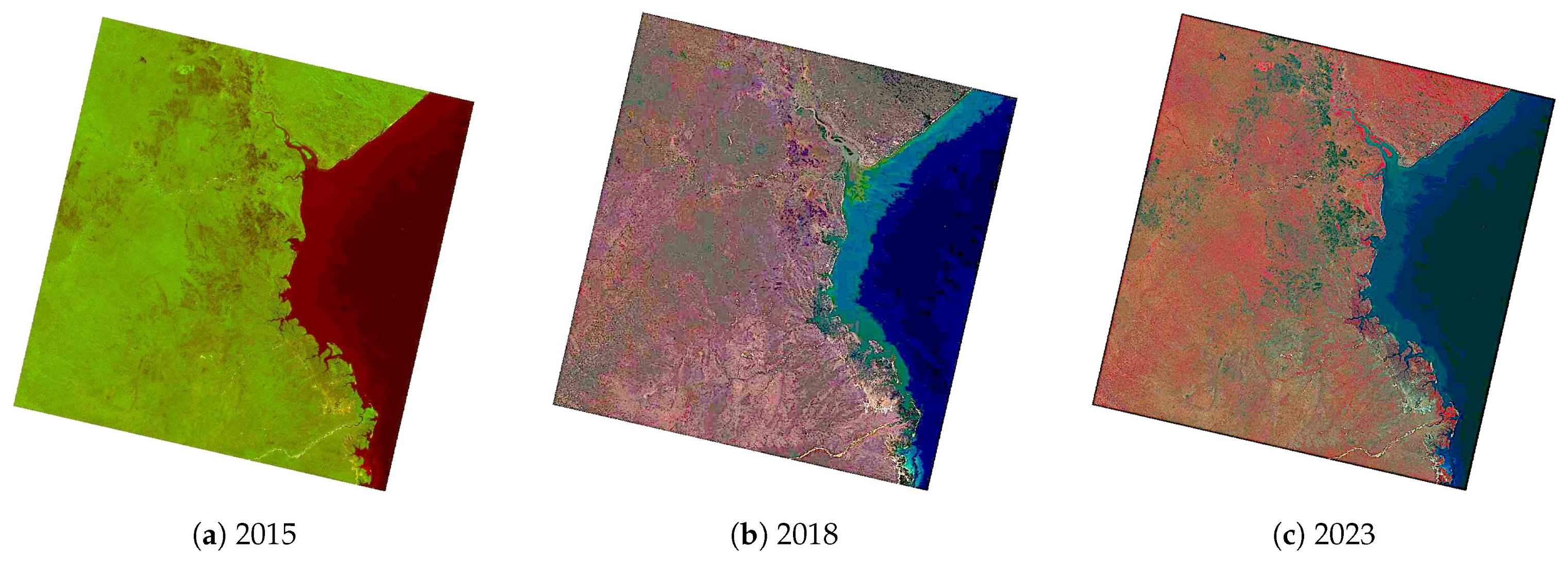
The color composites created using a combination of bands for false and natural color composites are shown in Figure 5 with the case of an image from 2015. The image dates were distributed throughout the important stages of the vegetation growth period in order to obtain temporal profiles of each kind of land cover type to analyze the separability among classes. The particular characteristics of Mozambique consists of its longitudinal extent, with the coastline stretching for ca. 2000 km, 11° S to 27° S. Moreover, the effects from tropical ocean currents were directed southwards along the length of the country influence environmental setting. Therefore, regional characteristics naturally differ within the country.
Weather patterns in Mozambique vary due to the global warming and increase in temperature. Nevertheless, the whole country broadly follows a southern African weather pattern: wet period with heavy rainy between November and March and dry period from April to late November. Since Mozambique has a tropical climate which has two distinct seasons, the images were taken during the dry period. Better cloudiness conditions and dense vegetation coverage were observed during dry season, as shown in the images.
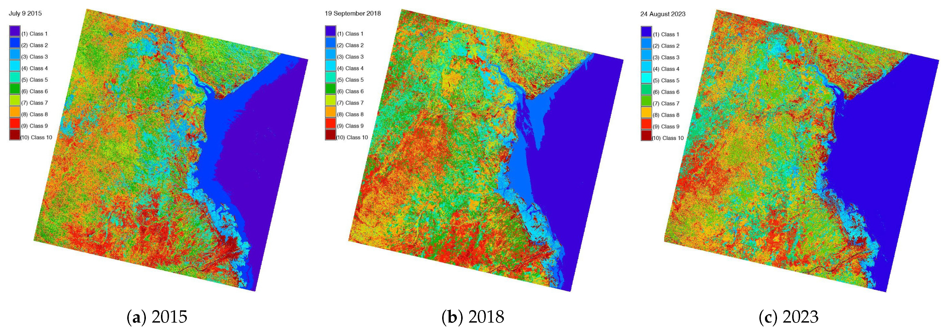
The results of the classification are shown in Figure 6. They were used as training data for the next step of random forest (RF) modeling, which requires seed data. The land cover types include the following classes: (1) mosaic cropland vegetation, (2) artificial surfaces and associated areas; (3) rain-fed croplands; (4) open grasslands; (5) sparse vegetation; (6) broad-leaved deciduous woodland; (7) mosaic forests, grassland and shrubland; (8) water areas; (9) needle-leaved deciduous evergreen forests; and (10) repeatedly or permanently flooded lands in brackish waters with broad-leaved forests or shrub lands. The coastal areas are characterized by grassland or woody vegetation distributed in areas of soil regularly flooded by fresh, brackish, or saline water.
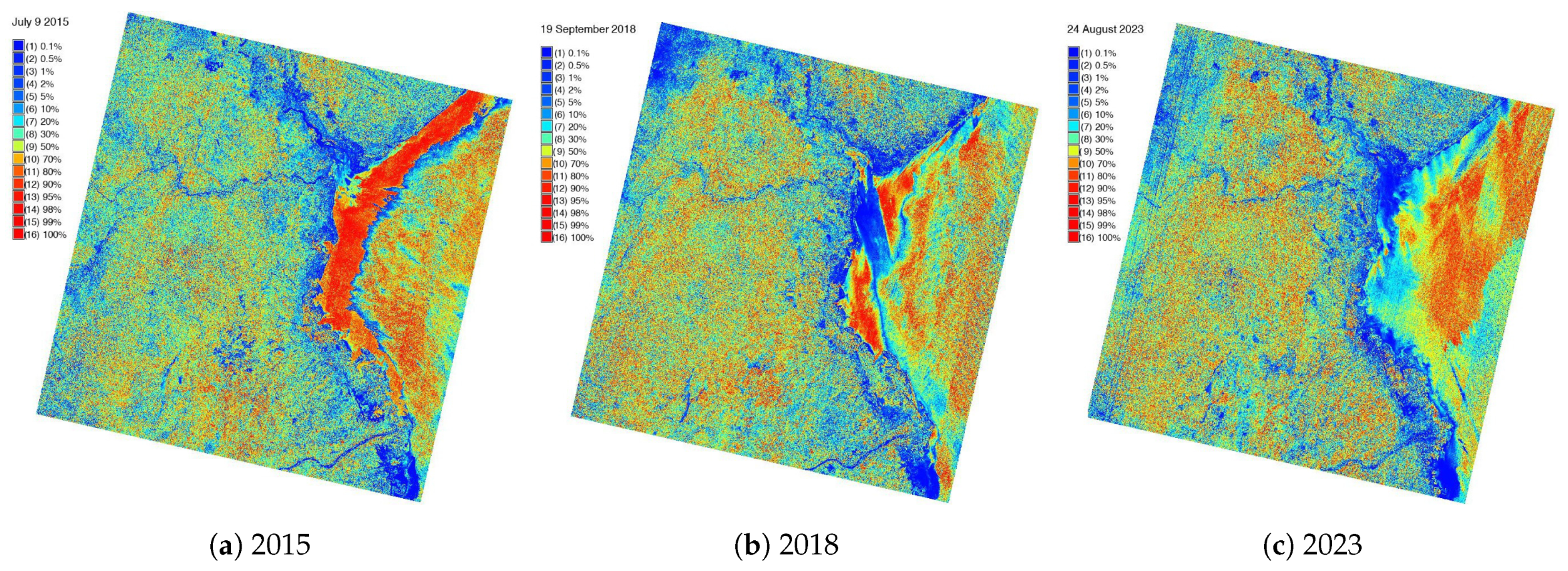
Figure 7 shows the result of a chi square test on the accuracy assessment of the classification on each discriminant result at various threshold levels of confidence. The aim of the chi square test is to determine if a correlation exists between two qualitative variables and if the existing associations are statistically significant. When using the maximum likelihood classification method to classify the land cover types, the accuracy of the classification depends on the quality of the training dataset and technical parameters of the satellite image. Thus, evaluating the accuracy analysis presents an important step in classification. The approach to accuracy assessments is based on the function embedded in ‘i.maxlik’, where pixels are classified according to the probability of their correct assignment to each land cover class.
As can be seen in Figure 7 showing reject threshold results, the lowest rejection values on the raster maps for three years—2015, 2018 and 2023—indicate the correctly classified pixels while the highest rejection values indicate the erroneously classified pixels. The analysis of Figure 7 indicates that the majority of the correctly indicated pixels belongs to the river and inner water classes as well as vegetation types with distinct separability properties. In contrast, the least secure pixels belong to the tidal region in the coastal waters due to the spectral properties of shelf water areas where pixels might be misclassified and with other land cover types due to the high similarity of spectral reflectance values.
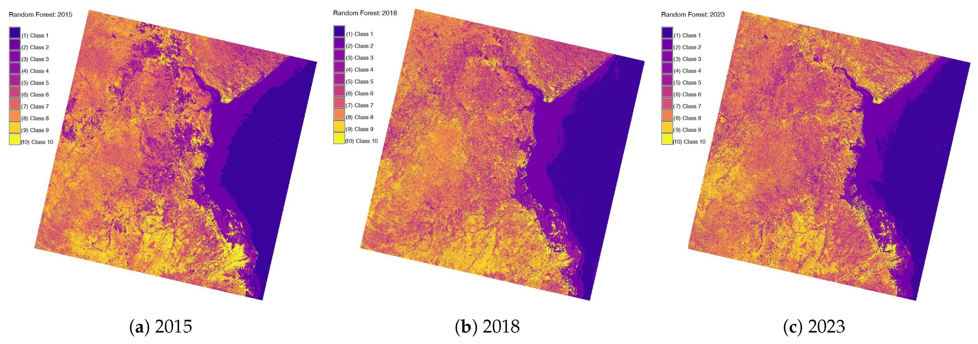
This method is suitable for providing a sufficient estimation on the accuracy of training samples that were used for the final steps of classification using random forest. The resulting images of the random forest classification of Landsat 8–9 OLI/TIRS images by the ML approach of GRASS GIS for the years 2015, 2018, and 2023 are presented in Figure 8.
Figure 8 shows the results of the land cover type classification of the coastal region of Mozambique performed using the RF classifier approach of the ML method in GRASS GIS. The land cover types in Mozambique were selected for random forest classification with the estimator settings tab, providing access to the most pertinent parameters. These affect the previously described algorithms, where landscape patches were classified using the maximum likelihood classifier. The embedded Scikit-Learn library of Python contents provide the estimator parameters that are supplied for classification. These parameters were tuned using a grid search in the Landsat raster maps by inputting multiple regressors. This enabled us to indicate the representativeness of the land cover classes, uniformity or heterogeneity of patches, and the classification of pixels located far from the edges of the raster scene.
The ML approach by the Scikit-Learn library of Python ensures that the confusion of image pixels is avoided as much as possible compared to traditional classification methods. Moreover, training pixels generated during clustering and used to perform the RF-based classification separated the images into clusters of pixels. These groups were used both as a decision tree training seed dataset for random forest classifiers and as a post-classification accuracy assessment. In this way, the RF method avoided biased reference information of the group of pixels.

5. Discussion

In this study, the ML method of random forest classification of GRASS GIS was applied for the processing and analysis of three Landsat 8–9 OLI/TIRS images with the aim of land cover mapping in the coastal region of the Bight of Sofala, Mozambique. Quantitative image processing and interpretation are not easy tasks due to the complex function of multiple factors. These include, for instance, technical parameters of the image (sun, sensor, and target geometry), regional environmental effects (cloudiness, wetness, heterogeneity, diversification and fragmentation of landscapes, topographic ruggedness, and slope curvature) as well as sensitivity to leaf characteristics [107]. The ML approach of GRASS GIS enabled us to perform a quantitative image classification using the random forest algorithm, which evaluated the similarity of pixels and assigned them into classes using the ‘r.learn.train’ module. The statistical information was obtained from the raster data analysis to represent the land cover types in Mozambique for the years 2015, 2018, and 2023.
Such an algorithm enabled us to model clusters of pixels, which were used to compare the climate effects that cause changes in land cover classes and lead to spatio-temporal landscape dynamics. This was achieved using the ensemble classification achieved by the random forest approach. Each tree in this ensemble was based on a random subsample of the training data that were initially obtained using the unsupervised classification as a part of data processing. This work is comparable with investigations performed by the authors of related works, for instance, those in [108,109].
Similar research [110,111,112] investigated the complementarities of the ML approach for mapping coastal regions using a set of multi-resolution imagery from the Sentinel-2 Multispectral Instrument (MSI) and Landsat-8 OLI. To continue these studies, the experiments on image processing using the random forest approach reported in this article investigated the landscape dynamics in the study area of eastern Mozambique. This was achieved using a randomly selected subset of the predictors available during each node split in the ML-based classification method of GRASS GIS. Other studies [113,114,115] used a neural network as a technical approach to the classification of vegetation and land cover types. Such a technique of remote sensing data processing aims to classify the land cover types using ML methods and reports high accuracy. Hence, we used the emerging technologies of scripts and programming algorithms for image processing through a set of GRASS GIS modules.
The demonstrated workflow was developed using a short series of the Landsat images. These images had various combinations of pixels which were evaluated by the ML methods to analyze the land cover changes using prediction analyses. Each tree of the algorithm produced a prediction. The final result of the image analysis was obtained by selecting the mean values across all of the trees in the Landsat image raster using computer vision. In other studies, a decision tree classifier was adopted to the RS data processing for automatic classification using diverse software. For instance, Ref. [116] used the ensemble techniques of boosting and consensus filtering of the training data to improve the quality of the training dataset. Ref. [117] compared the integrated use of the three classification schemes based on RF, DL neural network, and convolutional neural network to distinguish urban, natural, and heterogeneous landscape patches. Likewise, the ExtraTreesClassifier has been used as a variant of the GRASS GIS ML algorithm. Here, each node split during image processing includes the selected splitting rule, which is based on the most optimal solution.
Such optimization applied to several randomly generated thresholds by the random forest method presented advantages over the traditional unsupervised methods of image classification when generating classes for image classification. For instance, Ref. [118] reports that the parameter-adjusted decision tree ensembles and RF ensembles performed well for image segmentation and supervised and outperformed other approaches. Likewise, the updates in the algorithms were reported using the improved decision tree algorithm based on the fuzzy approach for a technical improvement in the performance [119]. Although the study presented here is not intended to suggest that scripting methods replace the traditional GIS, the integration of the scripting workflow of GRASS GIS with a satellite image analysis and cartographic plotting provides a more effective approach. This study demonstrated that the programming codes supplement the traditional cartographic methods used in the remote sensing software for monitoring coastal areas. Moreover, this work illustrated how the analysis of land cover changes can be visualized in the automatic way using ML algorithms of GRASS GIS.

6. Conclusions

The application of programming for RS data processing provides new perspectives in cartographic data processing. Such approaches are useful for mapping complex landscapes in the entanglement of human-based factors and environmental processes that affect coastal ecosystems. In view of this, the current study presented advanced mapping approaches to spatial analysis and visualization of the RS data. The use of the ML and intelligence classifiers of GRASS GIS increased the accuracy and precision of the produced thematic maps through the high level of automation. Moreover, it improved the performance of tasks using diversified modules and the application of RF algorithms for land cover classifications. The satellite images were classified using the unsupervised and supervised methods of the ML modules of GRASS GIS, including the random forest classifier.
The Bight of Sofala, located in the eastern coastal part of Mozambique, was selected as the test area due to the variability and high heterogeneity of landscapes with a complex mosaic of landscape patches. Ten types of land cover classes were identified on the Landsat satellite images collected in the years 2015, 2018, and 2023. The data were classified using the random forest algorithm of the machine learning (ML) methods supported by the Scikit-Learn library of Python integrated with GRASS GIS. The clustering approach of the machine-based classification was employed for training and validation of the result of the RF classification. The benefits of the RS data used for environmental monitoring consist of the fact that they provide an efficient way to map and visualize remotely located regions such as coastal regions in East Africa. Scripts used as a methodological benchmark of the automated image processing and cartographic workflow enabled us to focus on the analysis of the coastal landscapes of Mozambique.
The coastal region of the Bight of Sofala and its surroundings were analyzed using the classified series of satellite images in Landsat with the applied methods of automated data analysis of the ML approach. The advantage of the proposed algorithms of GRASS GIS scripts consists of their repeatability and applicability. The use of the supervised classification by the ‘r.learn.train’ module can be extended to other regions and environmental applications where satellite image processing is required. In this way, the ML method classification of landscapes can be applied in studies that use a multi-temporal set of images. The advanced approach of the GRASS GIS scripts was introduced to evaluate the environmental properties of the coastal landscapes of Mozambique. Changes in land cover types caused by climate effects in East Africa were visualized using image processing by the GRASS GIS modules ‘r.learn.train’ , ‘i.cluster’, ‘i.maxlik’, and other auxiliary modules.
The results visualize the dynamical behavior of land cover types in the coastal landscapes of Mozambique caused by climate effects, which act as drivers for desertification and land degradation in the coastal ecosystems of East Africa. We also discussed the ways in which the ML methods technically contrast with the traditional methods of the unsupervised classification. For instance, these use k-means clustering as an approach to image analysis for evaluating landscape changes using a series of images taken on different dates. Thus, it has been demonstrated that the ML approach of GRASS GIS has high automation in the sequential image processing workflow, which enables the effective use of RS data for environmental monitoring of coastal regions.

Funding

This research received no external funding.

Institutional Review Board Statement

Not applicable.

Informed Consent Statement

Not applicable.

Data Availability Statement

The data are contained within the article.

Acknowledgments

The authors thank the reviewers for reading and reviewing this manuscript.

Conflicts of Interest

The author declares no conflicts of interest.

Abbreviations

The following abbreviations are used in this manuscript:
AVHRRAdvanced Very High Resolution Radiometer
CCToolsCooperative Computing Tools
DCWDigital Chart of the World
DLDeep Learning
DNDigital Numbers
FAOFood and Agriculture Organization
GDALGeospatial Data Abstraction Library
GEBCOGeneral Bathymetric Chart of the Oceans
GRASSGeographic Resources Analysis Support System
GISGeographic Information System
GCCGNU Compiler Collection
GMTGeneric Mapping Tools
Landsat OLI/TIRSLandsat Operational Land Imager and Thermal Infrared Sensor
Landsat MSSMultispectral Scanner
Landsat TMLandsat Thematic Mapper
MLMachine Learning
NIRNear Infrared
NOAANational Oceanic and Atmospheric Administration
RFRandom Forest
Sentinel MSISentinel Multispectral Instrument
SPOTSatellite Pour l’Observation de la Terre
SRTMShuttle Radar Topography Mission
SWIRShortwave Infrared
ToARTop-of-Atmosphere Radiances
USGSUnited States Geological Survey
UTMUniversal Transverse Mercator

References

  1. Fagan, M.E.; DeFries, R.S. Remote Sensing and Image Processing. In Encyclopedia of Biodiversity, 3rd ed.; Scheiner, S.M., Ed.; Academic Press: Oxford, UK, 2024; pp. 432–445. [Google Scholar] [CrossRef]
  2. Loeb, N.G. Satellites and Satellite Remote Sensing|Earth’s Radiation Budget. In Reference Module in Earth Systems and Environmental Sciences; Elsevier: Amsterdam, The Netherlands, 2023. [Google Scholar] [CrossRef]
  3. Brenning, A. Spatial cross-validation and bootstrap for the assessment of prediction rules in remote sensing: The R package sperrorest. In Proceedings of the 2012 IEEE International Geoscience and Remote Sensing Symposium, Munich, Germany, 22–27 July 2012; pp. 5372–5375. [Google Scholar] [CrossRef]
  4. Lemenkova, P.; Debeir, O. Recognizing the Wadi Fluvial Structure and Stream Network in the Qena Bend of the Nile River, Egypt, on Landsat 8-9 OLI Images. Information 2023, 14, 249. [Google Scholar] [CrossRef]
  5. Lemenkova, P.; Debeir, O. Time Series Analysis of Landsat Images for Monitoring Flooded Areas in the Inner Niger Delta, Mali. Artif. Satell. 2023, 58, 278–313. [Google Scholar] [CrossRef]
  6. Zhao, D.; Huang, J.; Li, Z.; Yu, G.; Shen, H. Dynamic monitoring and analysis of chlorophyll-a concentrations in global lakes using Sentinel-2 images in Google Earth Engine. Sci. Total Environ. 2024, 912, 169152. [Google Scholar] [CrossRef] [PubMed]
  7. Lemenkova, P. Sentinel-2 for High Resolution Mapping of Slope-Based Vegetation Indices Using Machine Learning by SAGA GIS. Transylv. Rev. Syst. Ecol. Res. 2020, 22, 17–34. [Google Scholar] [CrossRef]
  8. Choudhary, K.; Shi, W.; Dong, Y.; Paringer, R. Random Forest for rice yield mapping and prediction using Sentinel-2 data with Google Earth Engine. Adv. Space Res. 2022, 70, 2443–2457. [Google Scholar] [CrossRef]
  9. Ji, L.; Brown, J.F. Effect of NOAA satellite orbital drift on AVHRR-derived phenological metrics. Int. J. Appl. Earth Obs. Geoinf. 2017, 62, 215–223. [Google Scholar] [CrossRef]
  10. Zhan, C.; Liang, S. Improved estimation of the global top-of-atmosphere albedo from AVHRR data. Remote Sens. Environ. 2022, 269, 112836. [Google Scholar] [CrossRef]
  11. Fensholt, R.; Rasmussen, K.; Nielsen, T.T.; Mbow, C. Evaluation of earth observation based long term vegetation trends—Intercomparing NDVI time series trend analysis consistency of Sahel from AVHRR GIMMS, Terra MODIS and SPOT VGT data. Remote Sens. Environ. 2009, 113, 1886–1898. [Google Scholar] [CrossRef]
  12. Chen, C.; Yang, X.; Jiang, S.; Liu, Z. Mapping and spatiotemporal dynamics of land-use and land-cover change based on the Google Earth Engine cloud platform from Landsat imagery: A case study of Zhoushan Island, China. Heliyon 2023, 9, e19654. [Google Scholar] [CrossRef]
  13. Lemenkova, P. Using open-source software GRASS GIS for analysis of the environmental patterns in Lake Chad, Central Africa. Die Bodenkult. J. Land Manag. Food Environ. 2023, 74, 49–64. [Google Scholar] [CrossRef]
  14. Lemesios, I.; Petropoulos, G.P. Vegetation regeneration dynamics of a natural mediterranean ecosystem following a wildfire exploiting the LANDSAT archive, google earth engine and geospatial analysis techniques. Remote. Sens. Appl. Soc. Environ. 2024, 34, 101153. [Google Scholar] [CrossRef]
  15. Senay, G.B.; Friedrichs, M.; Morton, C.; Parrish, G.E.; Schauer, M.; Khand, K.; Kagone, S.; Boiko, O.; Huntington, J. Mapping actual evapotranspiration using Landsat for the conterminous United States: Google Earth Engine implementation and assessment of the SSEBop model. Remote Sens. Environ. 2022, 275, 113011. [Google Scholar] [CrossRef]
  16. Lemenkova, P.; Debeir, O. Environmental mapping of Burkina Faso using TerraClimate data and satellite images by GMT and R scripts. Adv. Geod. Geoinf. 2023, 72, e45. [Google Scholar] [CrossRef]
  17. Xie, Y.; Li, J.; Wulan, T.; Zheng, Y.; Shen, Z. Scale dependence of forest fragmentation and its climate sensitivity in a semi-arid mountain: Comparing Landsat, Sentinel and Google Earth data. Geogr. Sustain. 2023, in press. [Google Scholar] [CrossRef]
  18. Radeloff, V.C.; Roy, D.P.; Wulder, M.A.; Anderson, M.; Cook, B.; Crawford, C.J.; Friedl, M.; Gao, F.; Gorelick, N.; Hansen, M.; et al. Need and vision for global medium-resolution Landsat and Sentinel-2 data products. Remote Sens. Environ. 2024, 300, 113918. [Google Scholar] [CrossRef]
  19. Giri, C.; Zhu, Z.; Reed, B. A comparative analysis of the Global Land Cover 2000 and MODIS land cover data sets. Remote Sens. Environ. 2005, 94, 123–132. [Google Scholar] [CrossRef]
  20. Wang, Y.; Sun, Y.; Cao, X.; Wang, Y.; Zhang, W.; Cheng, X. A review of regional and Global scale Land Use/Land Cover (LULC) mapping products generated from satellite remote sensing. ISPRS J. Photogramm. Remote Sens. 2023, 206, 311–334. [Google Scholar] [CrossRef]
  21. He, T.; Liang, S.; Wang, D.; Cao, Y.; Gao, F.; Yu, Y.; Feng, M. Evaluating land surface albedo estimation from Landsat MSS, TM, ETM+, and OLI data based on the unified direct estimation approach. Remote Sens. Environ. 2018, 204, 181–196. [Google Scholar] [CrossRef]
  22. Hussain, S.; Mubeen, M.; Karuppannan, S. Land use and land cover (LULC) change analysis using TM, ETM+ and OLI Landsat images in district of Okara, Punjab, Pakistan. Phys. Chem. Earth Parts A/B/C 2022, 126, 103117. [Google Scholar] [CrossRef]
  23. Estoque, R.C.; Murayama, Y. Classification and change detection of built-up lands from Landsat-7 ETM+ and Landsat-8 OLI/TIRS imageries: A comparative assessment of various spectral indices. Ecol. Indic. 2015, 56, 205–217. [Google Scholar] [CrossRef]
  24. Wulder, M.A.; Roy, D.P.; Radeloff, V.C.; Loveland, T.R.; Anderson, M.C.; Johnson, D.M.; Healey, S.; Zhu, Z.; Scambos, T.A.; Pahlevan, N.; et al. Fifty years of Landsat science and impacts. Remote Sens. Environ. 2022, 280, 113195. [Google Scholar] [CrossRef]
  25. Ferreira, M.A.; Andrade, F.; Bandeira, S.O.; Cardoso, P.; Mendes, R.N.; Paula, J. Analysis of cover change (1995–2005) of Tanzania/Mozambique trans-boundary mangroves using Landsat imagery. Aquat. Conserv. Mar. Freshw. Ecosyst. 2009, 19, S38–S45. [Google Scholar] [CrossRef]
  26. Montfort, F.; Bégué, A.; Leroux, L.; Blanc, L.; Gond, V.; Cambule, A.H.; Remane, I.A.D.; Grinand, C. From land productivity trends to land degradation assessment in Mozambique: Effects of climate, human activities and stakeholder definitions. Land Degrad. Dev. 2021, 32, 49–65. [Google Scholar] [CrossRef]
  27. Fatoyinbo, T.E.; Simard, M.; Washington-Allen, R.A.; Shugart, H.H. Landscape-scale extent, height, biomass, and carbon estimation of Mozambique’s mangrove forests with Landsat ETM+ and Shuttle Radar Topography Mission elevation data. J. Geophys. Res. Biogeosci. 2008, 113, G02S06. [Google Scholar] [CrossRef]
  28. Ribeiro, N.S.; Saatchi, S.S.; Shugart, H.H.; Washington-Allen, R.A. Aboveground biomass and leaf area index (LAI) mapping for Niassa Reserve, northern Mozambique. J. Geophys. Res. Biogeosci. 2008, 113, G02S02. [Google Scholar] [CrossRef]
  29. Li, F.; Yigitcanlar, T.; Nepal, M.; Nguyen, K.; Dur, F. Machine learning and remote sensing integration for leveraging urban sustainability: A review and framework. Sustain. Cities Soc. 2023, 96, 104653. [Google Scholar] [CrossRef]
  30. Pham, T.D.; Ha, N.T.; Saintilan, N.; Skidmore, A.; Phan, D.C.; Le, N.N.; Viet, H.L.; Takeuchi, W.; Friess, D.A. Advances in Earth observation and machine learning for quantifying blue carbon. Earth-Sci. Rev. 2023, 243, 104501. [Google Scholar] [CrossRef]
  31. Han, W.; Zhang, X.; Wang, Y.; Wang, L.; Huang, X.; Li, J.; Wang, S.; Chen, W.; Li, X.; Feng, R.; et al. A survey of machine learning and deep learning in remote sensing of geological environment: Challenges, advances, and opportunities. ISPRS J. Photogramm. Remote Sens. 2023, 202, 87–113. [Google Scholar] [CrossRef]
  32. Khan, A.; Vibhute, A.D.; Mali, S.; Patil, C. A systematic review on hyperspectral imaging technology with a machine and deep learning methodology for agricultural applications. Ecol. Inform. 2022, 69, 101678. [Google Scholar] [CrossRef]
  33. Mullissa, A.; Reiche, J.; Herold, M. Deep learning and automatic reference label harvesting for Sentinel-1 SAR-based rapid tropical dry forest disturbance mapping. Remote Sens. Environ. 2023, 298, 113799. [Google Scholar] [CrossRef]
  34. Lemenkova, P. Tanzania Craton, Serengeti Plain and Eastern Rift Valley: Mapping of geospatial data by scripting techniques. Est. J. Earth Sci. 2022, 71, 61–79. [Google Scholar] [CrossRef]
  35. Lemenkova, P.; Debeir, O. Satellite Image Processing by Python and R Using Landsat 9 OLI/TIRS and SRTM DEM Data on Côte d’Ivoire, West Africa. J. Imaging 2022, 8, 317. [Google Scholar] [CrossRef] [PubMed]
  36. Liu, J.; Qiu, Z.; Feng, J.; Wong, K.P.; Tsou, J.Y.; Wang, Y.; Zhang, Y. Monitoring Total Suspended Solids and Chlorophyll-a Concentrations in Turbid Waters: A Case Study of the Pearl River Estuary and Coast Using Machine Learning. Remote Sens. 2023, 15, 5559. [Google Scholar] [CrossRef]
  37. Wu, Y.; Jiang, N.; Xu, Y.; Yeh, T.K.; Xu, T.; Wang, Y.; Su, W. Improving the capability of water vapor retrieval from Landsat 8 using ensemble machine learning. Int. J. Appl. Earth Obs. Geoinf. 2023, 122, 103407. [Google Scholar] [CrossRef]
  38. Chen, J.; Huang, J.; Zhang, X.; Chen, J.; Chen, X. Monitoring total suspended solids concentration in Poyang Lake via machine learning and Landsat images. J. Hydrol. Reg. Stud. 2023, 49, 101499. [Google Scholar] [CrossRef]
  39. Wu, Y.; Pan, J. Detecting Changes in Impervious Surfaces Using Multi-Sensor Satellite Imagery and Machine Learning Methodology in a Metropolitan Area. Remote Sens. 2023, 15, 5387. [Google Scholar] [CrossRef]
  40. Lin, Y.; Li, L.; Yu, J.; Hu, Y.; Zhang, T.; Ye, Z.; Syed, A.; Li, J. An optimized machine learning approach to water pollution variation monitoring with time-series Landsat images. Int. J. Appl. Earth Obs. Geoinf. 2021, 102, 102370. [Google Scholar] [CrossRef]
  41. Liao, Q. Intelligent classification model of land resource use using deep learning in remote sensing images. Ecol. Model. 2023, 475, 110231. [Google Scholar] [CrossRef]
  42. Guo, J.; Xu, Q.; Zeng, Y.; Liu, Z.; Zhu, X.X. Nationwide urban tree canopy mapping and coverage assessment in Brazil from high-resolution remote sensing images using deep learning. ISPRS J. Photogramm. Remote Sens. 2023, 198, 1–15. [Google Scholar] [CrossRef]
  43. Zhang, Q.; Wang, G.; Wang, G.; Song, W.; Wei, X.; Hu, Y. Identifying Winter Wheat Using Landsat Data Based on Deep Learning Algorithms in the North China Plain. Remote Sens. 2023, 15, 5121. [Google Scholar] [CrossRef]
  44. Dou, P.; Shen, H.; Li, Z.; Guan, X. Time series remote sensing image classification framework using combination of deep learning and multiple classifiers system. Int. J. Appl. Earth Obs. Geoinf. 2021, 103, 102477. [Google Scholar] [CrossRef]
  45. Boulila, W.; Sellami, M.; Driss, M.; Al-Sarem, M.; Safaei, M.; Ghaleb, F.A. RS-DCNN: A novel distributed convolutional-neural-networks based-approach for big remote-sensing image classification. Comput. Electron. Agric. 2021, 182, 106014. [Google Scholar] [CrossRef]
  46. Lin, J.; Zhao, Y.; Wang, S.; Tang, Y. A robust training method for object detectors in remote sensing image. Displays 2024, 81, 102618. [Google Scholar] [CrossRef]
  47. Roberts, J.; Mwangi, R.; Mukabi, F.; Njui, J.; Nzioka, K.; Ndambiri, J.; Bispo, P.; Espirito-Santo, F.; Gou, Y.; Johnson, S.; et al. Pyeo: A Python package for near-real-time forest cover change detection from Earth observation using machine learning. Comput. Geosci. 2022, 167, 105192. [Google Scholar] [CrossRef]
  48. Guo, Z.; Guo, F.; Zhang, Y.; He, J.; Li, G.; Yang, Y.; Zhang, X. A python system for regional landslide susceptibility assessment by integrating machine learning models and its application. Heliyon 2023, 9, e21542. [Google Scholar] [CrossRef] [PubMed]
  49. Redoloza, F.S.; Williamson, T.N.; Headman, A.O.; Allred, B.J. Machine-learning model to delineate sub-surface agricultural drainage from satellite imagery. J. Environ. Qual. 2023, 52, 907–921. [Google Scholar] [CrossRef] [PubMed]
  50. GRASS Development Team. Geographic Resources Analysis Support System (GRASS GIS) Software, Version 8.2.; Open Source Geospatial Foundation: Beaverton, OR, USA, 2022. [Google Scholar]
  51. Strigaro, D.; Moretti, M.; Mattavelli, M.; Frigerio, I.; Amicis, M.D.; Maggi, V. A GRASS GIS module to obtain an estimation of glacier behavior under climate change: A pilot study on Italian glacier. Comput. Geosci. 2016, 94, 68–76. [Google Scholar] [CrossRef]
  52. Lemenkova, P. Monitoring Seasonal Fluctuations in Saline Lakes of Tunisia Using Earth Observation Data Processed by GRASS GIS. Land 2023, 12, 1995. [Google Scholar] [CrossRef]
  53. Jasiewicz, J. A new GRASS GIS fuzzy inference system for massive data analysis. Comput. Geosci. 2011, 37, 1525–1531. [Google Scholar] [CrossRef]
  54. Lemenkova, P. A GRASS GIS Scripting Framework for Monitoring Changes in the Ephemeral Salt Lakes of Chotts Melrhir and Merouane, Algeria. Appl. Syst. Innov. 2023, 6, 61. [Google Scholar] [CrossRef]
  55. Jasiewicz, J.; Metz, M. A new GRASS GIS toolkit for Hortonian analysis of drainage networks. Comput. Geosci. 2011, 37, 1162–1173. [Google Scholar] [CrossRef]
  56. Lemenkova, P. Image Segmentation of the Sudd Wetlands in South Sudan for Environmental Analytics by GRASS GIS Scripts. Analytics 2023, 2, 745–780. [Google Scholar] [CrossRef]
  57. Rocchini, D.; Delucchi, L.; Bacaro, G.; Cavallini, P.; Feilhauer, H.; Foody, G.M.; He, K.S.; Nagendra, H.; Porta, C.; Ricotta, C.; et al. Calculating landscape diversity with information-theory based indices: A GRASS GIS solution. Ecol. Inform. 2013, 17, 82–93. [Google Scholar] [CrossRef]
  58. Hofierka, J.; Mitášová, H.; Neteler, M. Chapter 17 Geomorphometry in GRASS GIS. In Geomorphometry; Hengl, T., Reuter, H.I., Eds.; Developments in Soil Science Series; Elsevier: Amsterdam, The Netherlands, 2009; Volume 33, pp. 387–410. [Google Scholar] [CrossRef]
  59. Pedregosa; Varoquaux, G.; Gramfort, A.; Michel, V.; Thirion, B. Scikit-learn: Machine Learning in Python. J. Mach. Learn. Res. 2011, 12, 2825–2830. [Google Scholar]
  60. Wessel, P.; Luis, J.F.; Uieda, L.; Scharroo, R.; Wobbe, F.; Smith, W.H.F.; Tian, D. The Generic Mapping Tools Version 6. Geochem. Geophys. Geosystems 2019, 20, 5556–5564. [Google Scholar] [CrossRef]
  61. Mucova, S.A.R.; Filho, W.L.; Azeiteiro, U.M.; Pereira, M.J. Assessment of land use and land cover changes from 1979 to 2017 and biodiversity & land management approach in Quirimbas National Park, Northern Mozambique, Africa. Glob. Ecol. Conserv. 2018, 16, e00447. [Google Scholar] [CrossRef]
  62. Jansen, L.J.; Bagnoli, M.; Focacci, M. Analysis of land-cover/use change dynamics in Manica Province in Mozambique in a period of transition (1990–2004). For. Ecol. Manag. 2008, 254, 308–326. [Google Scholar] [CrossRef]
  63. Bacar, F.F.; Faque, H.B. Forest holds high rodent diversity than other habitats under a rapidly changing and fragmenting landscape in Quirimbas National Park, Mozambique. Acta Ecol. Sin. 2023. [Google Scholar] [CrossRef]
  64. Dunham, K.M. Biomass dynamics of herbaceous vegetation in Zambezi riverine woodlands. Afr. J. Ecol. 1990, 28, 200–212. [Google Scholar] [CrossRef]
  65. Simasiku, E.K.; Hay, C.; Abah, J. Effect of water level and water quality on small-sized and juvenile fish assemblages in the littoral zones of the Zambezi/Chobe floodplain. Afr. J. Ecol. 2021, 59, 436–448. [Google Scholar] [CrossRef]
  66. Dunham, K.M. Phenology of Acacia albida trees in Zambezi riverine woodlands. Afr. J. Ecol. 1991, 29, 118–129. [Google Scholar] [CrossRef]
  67. Mbumwae, L.L. Environmental management of the Zambezi river system. Regul. Rivers Res. Manag. 1988, 2, 553–557. [Google Scholar] [CrossRef]
  68. Nehama, F.P.; Reason, C.J. The wind-driven response of the Zambezi River plume along the Sofala Bank: A numerical model study. Reg. Stud. Mar. Sci. 2021, 46, 101891. [Google Scholar] [CrossRef]
  69. Gope, E.T.; Sass-Klaassen, U.G.W.; Irvine, K.; Beevers, L.; Hes, E.M.A. Effects of flow alteration on Apple-ring Acacia (Faidherbia albida) stands, Middle Zambezi floodplains, Zimbabwe. Ecohydrology 2015, 8, 922–934. [Google Scholar] [CrossRef]
  70. Moore, A.E.; Cotterill, F.P.; Main, M.P.; Williams, H.B. The Zambezi: Origins and Legacies of Earth’s Oldest River System. In Large Rivers; John Wiley & Sons, Ltd.: Hoboken, NJ, USA, 2022; Chapter 16; pp. 457–487. [Google Scholar] [CrossRef]
  71. Leal, M.; Sá, C.; Nordez, S.; Brotas, V.; Paula, J. Distribution and vertical dynamics of planktonic communities at Sofala Bank, Mozambique. Estuar. Coast. Shelf Sci. 2009, 84, 605–616. [Google Scholar] [CrossRef]
  72. Malauene, B.S.; Moloney, C.L.; Lett, C.; Roberts, M.J.; Marsac, F.; Penven, P. Impact of offshore eddies on shelf circulation and river plumes of the Sofala Bank, Mozambique Channel. J. Mar. Syst. 2018, 185, 1–12. [Google Scholar] [CrossRef]
  73. Malauene, B.S.; Lett, C.; Marsac, F.; Roberts, M.J.; Brito, A.; Abdula, S.; Moloney, C.L. Spawning areas of two shallow-water penaeid shrimps (Penaeus indicus and Metapenaeus monoceros) on the Sofala Bank, Mozambique. Estuar. Coast. Shelf Sci. 2021, 253, 107268. [Google Scholar] [CrossRef]
  74. Jokar Arsanjani, J.; Fibæk, C.S.; Vaz, E. Development of a cellular automata model using open source technologies for monitoring urbanisation in the global south: The case of Maputo, Mozambique. Habitat Int. 2018, 71, 38–48. [Google Scholar] [CrossRef]
  75. De Sousa, L.P.; Brito, A.; Abdula, S.; Caputi, N. Research assessment for the management of the industrial shallow-water multi-species shrimp fishery in Sofala Bank in Mozambique. Fish. Res. 2006, 77, 207–219. [Google Scholar] [CrossRef]
  76. Miguel, J.J. On optimal choice of delay equations to model shrimp population dynamics in Sofala Bank, Mozambique. Nonlinear Anal. Real World Appl. 2003, 4, 365–371. [Google Scholar] [CrossRef]
  77. Gammelsrød, T. Variation in shrimp abundance on the Sofala Bank, Mozambique, and its relation to the Zambezi River runoff. Estuar. Coast. Shelf Sci. 1992, 35, 91–103. [Google Scholar] [CrossRef]
  78. Nhangumbe, M.; Nascetti, A.; Georganos, S.; Ban, Y. Supervised and unsupervised machine learning approaches using Sentinel data for flood mapping and damage assessment in Mozambique. Remote Sens. Appl. Soc. Environ. 2023, 32, 101015. [Google Scholar] [CrossRef]
  79. Salvucci, V.; Santos, R. Vulnerability to Natural Shocks: Assessing the Short-Term Impact on Consumption and Poverty of the 2015 Flood in Mozambique. Ecol. Econ. 2020, 176, 106713. [Google Scholar] [CrossRef]
  80. Gall, M. Where to Go? Strategic Modelling of Access to Emergency Shelters in Mozambique. Disasters 2004, 28, 82–97. [Google Scholar] [CrossRef] [PubMed]
  81. Come, J.; Peer, N.; Nhamussua, J.L.; Miranda, N.A.; Macamo, C.C.; Cabral, A.S.; Madivadua, H.; Zacarias, D.; Narciso, J.; Snow, B. A socio-ecological survey in Inhambane Bay mangrove ecosystems: Biodiversity, livelihoods, and conservation. Ocean Coast. Manag. 2023, 244, 106813. [Google Scholar] [CrossRef]
  82. Fichtner, F.; Mandery, N.; Wieland, M.; Groth, S.; Martinis, S.; Riedlinger, T. Time-series analysis of Sentinel-1/2 data for flood detection using a discrete global grid system and seasonal decomposition. Int. J. Appl. Earth Obs. Geoinf. 2023, 119, 103329. [Google Scholar] [CrossRef]
  83. Bofana, J.; Zhang, M.; Wu, B.; Zeng, H.; Nabil, M.; Zhang, N.; Elnashar, A.; Tian, F.; da Silva, J.M.; Botão, A.; et al. How long did crops survive from floods caused by Cyclone Idai in Mozambique detected with multi-satellite data. Remote Sens. Environ. 2022, 269, 112808. [Google Scholar] [CrossRef]
  84. Guldemond, R.A.R.; van Aarde, R.J. Forest patch size and isolation as drivers of bird species richness in Maputaland, Mozambique. J. Biogeogr. 2010, 37, 1884–1893. [Google Scholar] [CrossRef]
  85. Ramayanti, S.; Nur, A.S.; Syifa, M.; Panahi, M.; Achmad, A.R.; Park, S.; Lee, C.W. Performance comparison of two deep learning models for flood susceptibility map in Beira area, Mozambique. Egypt. J. Remote Sens. Space Sci. 2022, 25, 1025–1036. [Google Scholar] [CrossRef]
  86. Smith, H.E.; Ryan, C.M.; Vollmer, F.; Woollen, E.; Keane, A.; Fisher, J.A.; Baumert, S.; Grundy, I.M.; Carvalho, M.; Lisboa, S.N.; et al. Impacts of land use intensification on human wellbeing: Evidence from rural Mozambique. Glob. Environ. Chang. 2019, 59, 101976. [Google Scholar] [CrossRef]
  87. Lundgren, M.; Strandh, V. Navigating a double burden – Floods and social vulnerability in local communities in rural Mozambique. Int. J. Disaster Risk Reduct. 2022, 77, 103023. [Google Scholar] [CrossRef]
  88. Silva, J.A.; Loboda, T.; Strong, M. Examining aspiration’s imprint on the landscape: Lessons from Mozambique’s Limpopo National Park. Glob. Environ. Chang. 2018, 51, 43–53. [Google Scholar] [CrossRef]
  89. Martins, A.R.; Shackleton, C.M. The contribution of wild palms to the livelihoods and diversification of rural households in southern Mozambique. For. Policy Econ. 2022, 142, 102793. [Google Scholar] [CrossRef]
  90. Pittman, S.J.; Swanborn, D.J.; Connor, D.W.; Wright, D.J. Application of Estuarine and Coastal Classifications in Marine Spatial Management. In Reference Module in Earth Systems and Environmental Sciences; Elsevier: Amsterdam, The Netherlands, 2023. [Google Scholar] [CrossRef]
  91. Xi, W.; Du, S.; Wang, Y.C.; Zhang, X. A spatiotemporal cube model for analyzing satellite image time series: Application to land-cover mapping and change detection. Remote Sens. Environ. 2019, 231, 111212. [Google Scholar] [CrossRef]
  92. Abidi, A.; Ienco, D.; Abbes, A.B.; Farah, I.R. Combining 2D encoding and convolutional neural network to enhance land cover mapping from Satellite Image Time Series. Eng. Appl. Artif. Intell. 2023, 122, 106152. [Google Scholar] [CrossRef]
  93. Mohammadi, S.; Belgiu, M.; Stein, A. Improvement in crop mapping from satellite image time series by effectively supervising deep neural networks. ISPRS J. Photogramm. Remote Sens. 2023, 198, 272–283. [Google Scholar] [CrossRef]
  94. Namaganda, E.; Otsuki, K.; Steel, G. Understanding the cumulative socioenvironmental impacts of energy transition-induced extractivism in Mozambique: The role of mixed methods. J. Environ. Manag. 2023, 338, 117811. [Google Scholar] [CrossRef] [PubMed]
  95. Gemusse, U.; Cardoso-Fernandes, J.; Lima, A.; Teodoro, A. Identification of pegmatites zones in Muiane and Naipa (Mozambique) from Sentinel-2 images, using band combinations, band ratios, PCA and supervised classification. Remote Sens. Appl. Soc. Environ. 2023, 32, 101022. [Google Scholar] [CrossRef]
  96. Liang, M.; Duncanson, L.; Silva, J.A.; Sedano, F. Quantifying aboveground biomass dynamics from charcoal degradation in Mozambique using GEDI Lidar and Landsat. Remote Sens. Environ. 2023, 284, 113367. [Google Scholar] [CrossRef]
  97. Bey, A.; Jetimane, J.; Lisboa, S.N.; Ribeiro, N.; Sitoe, A.; Meyfroidt, P. Mapping smallholder and large-scale cropland dynamics with a flexible classification system and pixel-based composites in an emerging frontier of Mozambique. Remote Sens. Environ. 2020, 239, 111611. [Google Scholar] [CrossRef]
  98. Lemenkova, P. Mapping submarine geomorphology of the Philippine and Mariana trenches by an automated approach using GMT scripts. Proc. Latv. Acad. Sciences. Sect. B Nat. Exact Appl. Sci. 2022, 76, 258–266. [Google Scholar] [CrossRef]
  99. Lemenkova, P.; Debeir, O. Multispectral Satellite Image Analysis for Computing Vegetation Indices by R in the Khartoum Region of Sudan, Northeast Africa. J. Imaging 2023, 9, 98. [Google Scholar] [CrossRef] [PubMed]
  100. Lemenkova, P.; Debeir, O. R Libraries for Remote Sensing Data Classification by k-means Clustering and NDVI Computation in Congo River Basin, DRC. Appl. Sci. 2022, 12, 12554. [Google Scholar] [CrossRef]
  101. Lemenkova, P.; Debeir, O. GDAL and PROJ Libraries Integrated with GRASS GIS for Terrain Modelling of the Georeferenced Raster Image. Technologies 2023, 11, 46. [Google Scholar] [CrossRef]
  102. Lemenkova, P.; Debeir, O. Computing Vegetation Indices from the Satellite Images Using GRASS GIS Scripts for Monitoring Mangrove Forests in the Coastal Landscapes of Niger Delta, Nigeria. J. Mar. Sci. Eng. 2023, 11, 871. [Google Scholar] [CrossRef]
  103. Lemenkova, P. Mapping Climate Parameters over the Territory of Botswana Using GMT and Gridded Surface Data from TerraClimate. ISPRS Int. J. Geo-Inf. 2022, 11, 473. [Google Scholar] [CrossRef]
  104. Lemenkova, P. Handling Dataset with Geophysical and Geological Variables on the Bolivian Andes by the GMT Scripts. Data 2022, 7, 74. [Google Scholar] [CrossRef]
  105. Lemenkova, P. Console-Based Mapping of Mongolia Using GMT Cartographic Scripting Toolset for Processing TerraClimate Data. Geosciences 2022, 12, 140. [Google Scholar] [CrossRef]
  106. Lemenkova, P. Cartographic scripts for seismic and geophysical mapping of Ecuador. Geografie 2022, 127, 195–218. [Google Scholar] [CrossRef]
  107. Mitchard, E.T.A.; Saatchi, S.S.; Woodhouse, I.H.; Nangendo, G.; Ribeiro, N.S.; Williams, M.; Ryan, C.M.; Lewis, S.L.; Feldpausch, T.R.; Meir, P. Using satellite radar backscatter to predict above-ground woody biomass: A consistent relationship across four different African landscapes. Geophys. Res. Lett. 2009, 36, L23401. [Google Scholar] [CrossRef]
  108. Fernando, W.A.M.; Senanayake, I. Developing a two-decadal time-record of rice field maps using Landsat-derived multi-index image collections with a random forest classifier: A Google Earth Engine based approach. Inf. Process. Agric. 2023, in press. [Google Scholar] [CrossRef]
  109. Kolarik, N.; Shrestha, N.; Caughlin, T.; Brandt, J. Leveraging high resolution classifications and random forests for hindcasting decades of mesic ecosystem dynamics in the Landsat time series. Ecol. Indic. 2024, 158, 111445. [Google Scholar] [CrossRef]
  110. Bera, D.; Das Chatterjee, N.; Bera, S.; Ghosh, S.; Dinda, S. Comparative performance of Sentinel-2 MSI and Landsat-8 OLI data in canopy cover prediction using Random Forest model: Comparing model performance and tuning parameters. Adv. Space Res. 2023, 71, 4691–4709. [Google Scholar] [CrossRef]
  111. Yan, X.; Li, J.; Smith, A.R.; Yang, D.; Ma, T.; Su, Y. Rapid Land Cover Classification Using a 36-Year Time Series of Multi-Source Remote Sensing Data. Land 2023, 12, 2149. [Google Scholar] [CrossRef]
  112. Zhang, H.; Zhang, Y.; Liu, K.; Lan, S.; Gao, T.; Li, M. Winter wheat yield prediction using integrated Landsat 8 and Sentinel-2 vegetation index time-series data and machine learning algorithms. Comput. Electron. Agric. 2023, 213, 108250. [Google Scholar] [CrossRef]
  113. Mountrakis, G.; Heydari, S.S. Harvesting the Landsat archive for land cover land use classification using deep neural networks: Comparison with traditional classifiers and multi-sensor benefits. ISPRS J. Photogramm. Remote Sens. 2023, 200, 106–119. [Google Scholar] [CrossRef]
  114. Singh, M.; Tyagi, K.D. Pixel based classification for Landsat 8 OLI multispectral satellite images using deep learning neural network. Remote Sens. Appl. Soc. Environ. 2021, 24, 100645. [Google Scholar] [CrossRef]
  115. Zheng, Z.; Yang, B.; Liu, S.; Xia, J.; Zhang, X. Extraction of impervious surface with Landsat based on machine learning in Chengdu urban, China. Remote Sens. Appl. Soc. Environ. 2023, 30, 100974. [Google Scholar] [CrossRef]
  116. Brown de Colstoun, E.C.; Story, M.H.; Thompson, C.; Commisso, K.; Smith, T.G.; Irons, J.R. National Park vegetation mapping using multitemporal Landsat 7 data and a decision tree classifier. Remote Sens. Environ. 2003, 85, 316–327. [Google Scholar] [CrossRef]
  117. Vaidya, M.; Keskar, R.; Kotharkar, R. Classifying heterogeneous urban form into local climate zones using supervised learning and greedy clustering incorporating Landsat dataset. Urban Clim. 2024, 53, 101770. [Google Scholar] [CrossRef]
  118. Pasquarella, V.J.; Morreale, L.L.; Brown, C.F.; Kilbride, J.B.; Thompson, J.R. Not-so-random forests: Comparing voting and decision tree ensembles for characterizing partial harvest events. Int. J. Appl. Earth Obs. Geoinf. 2023, 125, 103561. [Google Scholar] [CrossRef]
  119. Al-Obeidat, F.; Al-Taani, A.T.; Belacel, N.; Feltrin, L.; Banerjee, N. A Fuzzy Decision Tree for Processing Satellite Images and Landsat Data. Procedia Comput. Sci. 2015, 52, 1192–1197. [Google Scholar] [CrossRef]
Figure 1. Study area in the coastal region of the Bight of Sofala, Mozambique is indicated by the cyan-colored rotated square. Mapping software: Generic Mapping Tools, version 6.4.0, creator: [60], location: Palisades, NY 10964, United States. (GMT). Map source: author.
Coasts 04 00008 g001
Figure 2. Land cover types in Mozambique according to the Food and Agriculture Organization (FAO) data. Mapping software: QGIS, version 3.34, creator: QGIS Development Team, location: London, England, U.K. Map source: author’s work.
Coasts 04 00008 g002
Figure 3. Workflow of the data processing. Diagram software: R, software version number 4.2.2, creator: R Core Team, location: Vienna, Austria. Source: author’s work.
Coasts 04 00008 g003
Figure 4. Landsat images on the coastal region of Beira, Mozambique: (a) 9 July 2015; (b) 19 September 2018; (c) 24 August 2023. The images show natural colors of the Landsat 8–9 OLI/TIRS.
Coasts 04 00008 g004
Figure 5. Color composites of the Landsat-8 OLI/TIRS image on 2015 on the coastal region of Beira, Mozambique: (a) Bands 7-5-3; (b) Bands 2-3-4; (c) Bands 3-4-5. Major band designations for the Landsat-8 are Band 1—coastal aerosol; Band 2—blue; Band 3—green; Band 4—red; Band 5—near infrared (NIR); Band 6—shortwave infrared (SWIR) 1; Band 7—shortwave infrared (SWIR) 2.
Coasts 04 00008 g005
Figure 6. Classified Landsat-8–9 OLI/TIRS images on the coastal region of Beira, Mozambique, partitioned into 10 classes using k-means clustering approach: (a) 2015; (b) 2018; (c) 2023.
Coasts 04 00008 g006
Figure 7. Accuracy assessment using the rejection probability for pixels classified using k-means clustering method for Landsat 8–9 OLI/TIRS images on the coastal region of Beira, Mozambique: (a) 2015; (b) 2018; (c) 2023.
Coasts 04 00008 g007
Figure 8. Random forest classification using machine learning (ML) approach of GRASS GIS for the Landsat 8–9 OLI/TIRS images on coastal region of Beira, Mozambique: (a) 2015; (b) 2018; (c) 2023.
Coasts 04 00008 g008
Table 1. Identifiers (ID) of the six Landsat 8–9 OLI/TIRS images on the study area of Mozambique, obtained from the EarthExplorer USGS repository.
DateLandsat Product Identifier L1Scene ID
9 July 2015LC08_L2SP_167074_20150709_20200909_02_T1LC81670742015190LGN01
19 September 2018LC08_L2SP_167074_20180919_20200830_02_T1LC81670742018262LGN00
24 August 2023LC09_L2SP_167074_20230824_20230826_02_T1LC91670742023236LGN00
Disclaimer/Publisher’s Note: The statements, opinions and data contained in all publications are solely those of the individual author(s) and contributor(s) and not of MDPI and/or the editor(s). MDPI and/or the editor(s) disclaim responsibility for any injury to people or property resulting from any ideas, methods, instructions or products referred to in the content.

