
Modelling the Effects of Oyster Tables on Estuarine Tidal Flow


Cerema, Direction Risques, Eau et Mer, HA, Laboratoire de Génie Côtier et Environnement (LGCE), 155 Rue Piuerre Bouguer, Technopôle Brest-Iroise, BP 5, 29280 Plouzané, France
Coasts 2023, 3(1), 2-23; https://doi.org/10.3390/coasts3010002
Submission received: 14 December 2022
/
Revised: 26 January 2023
/
Accepted: 27 January 2023
/
Published: 30 January 2023
Abstract
:Oyster farming may impact the estuarine tidal circulation with a series of effects on environmental conditions and cultures’ growth. Hydrodynamic numerical models set up in estuaries integrated the presence of oyster structures by simply increasing the bottom friction coefficient over farming areas. However, for elevated oyster tables in tidal environments, such default calibration ignored the temporal variations of the friction coefficient between the conditions of submerged or unsubmerged structures. Thus, an original formulation of the Chézy coefficient was here proposed to integrate these modulations. Assessed against measured and predicted vertical velocity profiles on a 1/2 scaled model, this formulation was implemented in a simulation of the tidal circulation within the Aber Wrac’h estuary (Brittany, France). Particular attention was dedicated to the changes induced on the current magnitudes and sediment transport. Oyster tables were found to impact current magnitudes in the vicinity of elevated structures, with major differences at times of local peak flood and ebb. These modifications were characterised by (i) a reduction of current magnitudes over oyster farming areas and (ii) a tidal-flow acceleration on both sides of these structures. Increased sediment transport was, therefore, expected in the vicinity of these cultures, with potential implications on seabed morphology and water quality.
1. Introduction
Considered as an alternative to overfishing, aquaculture in marine waters has developed significantly over the last decades to meet the need for greater self-sufficiency in food production, mainly resulting from population growth, rising income, and urbanization [1]. Thus, marine aquaculture output exceeds today’s wild capture fisheries by providing nearly of the global seafood production. One of the main drivers is the culture of molluscan shellfish, characterised by a steady increase since the mid-nineties [2,3,4]. However, such impressive evolution requires in-depth assessment tools liable to encompass the wide range of potential ecological effects induced by these aquacultures, including, among others, the removal of nutrients, trophic competition, or increased primary productivity and sedimentation [5].
This is one of the major concern of intertidal oyster cultivation whose spatial occupation (especially in estuarine environments) may conflict with a wide range of environmental, social, and economic concerns [6,7]. While being primarily located on tidal flats of estuaries, higher current velocities are, in most cases, desirable for the implementation of this aquaculture to increase food delivery, enhance biodeposits’ dispersal (e.g., waste particles produced by biological filtering), and improve marine waters’ quality. However, oyster aquaculture also impacts the hydrodynamic flow, leading to a series of effects and modifications on environmental parameters (including salinity, temperature, turbidity, food supply or oxygen) [8,9,10]. Moreover, these modifications may have wider ecosystem consequences on fish, seabirds, and marine mammals and, in return, impact the growth and survivability of oysters [11,12]. Hydrodynamic interactions are particularly noticeable for raised farming on elevated tables, where oysters are locked up in meshed plastic bags attached to steel trestles [13,14]. This elevated farming technique is widely exploited in intertidal areas of north-western European shelf seas (particularly in western Brittany and Normandy, France), as its limits the exposition to predators, reduces losses, and increases the productive capacity. However, it also introduces artificial obstacles to the tidal flow that may lead to decrease of velocity magnitudes, thus limiting the dispersal of particles (including pollutants and contaminants) in the water column and increasing the natural sedimentation process by several orders of magnitude around oyster tables [15].
A comprehensive understanding of these interactions, including a large-scale assessment of potential environmental effects, is, thus, fundamental to optimise the management of this type of aquaculture. A refined approach of these interactions requires three-dimensional numerical simulations, typically based on computational fluid dynamics (CFD) codes, liable to reproduce the development of boundary layers, and perturbations of flow and turbulence parameters over and below the oyster tables [16]. However, given the high computational cost, this type of numerical simulations could not reasonably be adopted to reproduce the hydrodynamic interactions within an oyster farm or investigate the large-scale environmental effects within an estuary. Simplified methods were, therefore, retained by integrating these structures with a modified hydraulic roughness coefficient over the areas covered by oyster tables. Thus, for large-scale applications covering a bay or an estuary, simulations relied on increased friction coefficients over oyster farming areas. Nevertheless, for elevated oyster tables in tidal environments, such default calibration ignored the temporal variations associated with tidal elevation [15]. Indeed, strong differences of the friction coefficient are expected whether the oyster structures are submerged or not, and these modulations may be particularly important in intertidal areas of macro-tidal environments, typically considered for the implementation of oyster farms. Moreover, as exhibited by Gaurier et al. [16], the velocity profile above submerged oyster tables can not be approached by a classical roughness law (based on a physical roughness length in the near wall region of the oyster bags) and requires to consider the flow interaction effects inside these bags.
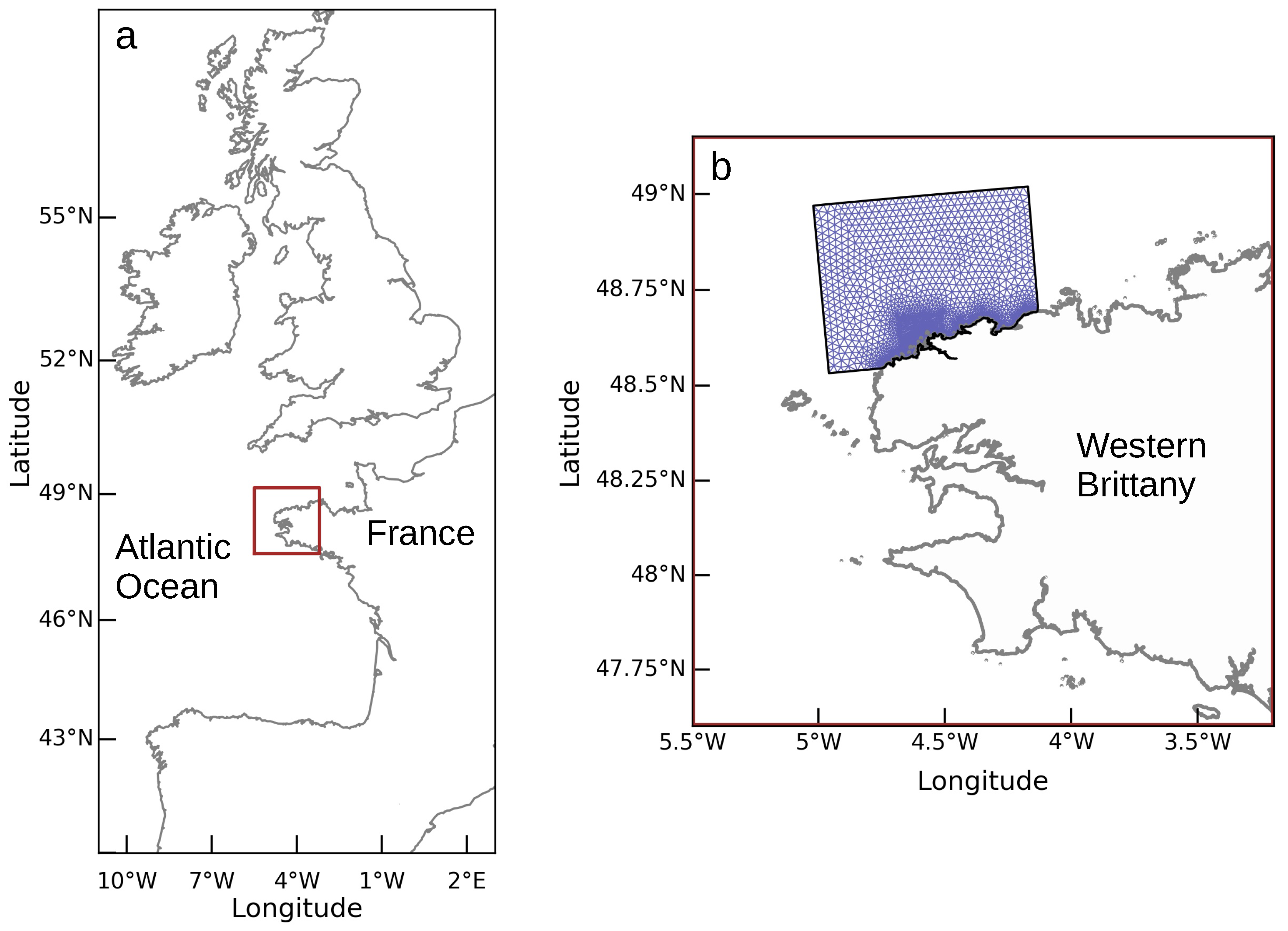
The present investigation complements these different studies by proposing an original simplified parametrisation of the friction coefficient over oyster farming areas dedicated to large-scale hydrodynamic simulations of the tidal circulation within bays or estuaries. This formulation integrates the flow interaction within oyster bags and effects of tidal elevation, thus drawing the line between the configurations of submerged and unsubmerged tables. This parametrisation was implemented as a revised Chézy coefficient in a depth-averaged tidal circulation model applied to an estuary with elevated oyster cultivation. The potential complementary effects of oyster tables on water quality (including especially filtering of sediments and other suspended particulate matter) were ignored, thus considering these effects negligible in intertidal farm sites that were regularly flushed over the successive tidal cycles [17]. The site of application is the Aber Wrac’h estuary in north-western Brittany (France), characterised by an access channel with mean water depth between 10 and 20 m that separates two inter-tidal areas covering the eastern and western sides with a series of oyster farms (Figure 1 and Figure 2).
With spring tidal range exceeding 6 m [18], this estuary is, furthermore, a typical macro-tidal environment of north-western Europe, sheltered from incoming waves by a series of islets and rocks off its mouth. The seabed is mainly composed of a mixture of very fine and muddy sands, with exceptions around islets where rock outcrops dominate [19]. Extending 7 km in length, with a width of around 2 km at its entrance, this estuary is, furthermore, relatively small, matching the great part of intertidal coastal areas considered for oyster farming. The site of application here considered may, thus, provide further insights for broader investigations in small intertidal estuaries integrating oyster tables. These insights may include the implementation of the hydrodynamic numerical model, the parametrisation of oyster farming areas, and the local and large-scale potential impacts of oyster tables.
The paper is organised as follows. After a description of the numerical model and the modified version of the Chézy coefficient over areas covered by oyster tables (Section 2), the predictions were assessed against a series of water depths and current measurements conducted in mean spring conditions in intertidal areas around oyster structures (Section 3.1). Simulations were exploited to investigate, for this real application, the sensitivity of model predictions to the parametrisation retained for the Chézy coefficient over oyster tables: the simple increase of the roughness parameter vs. the new formulation (Section 3.2). The attention was finally dedicated to changes induced by oyster tables on tidal current magnitudes, and two environmental factors liable to influence the production of oyster aquaculture: velocities exceedance over a given threshold and potential sediment transport (Section 3.3).
2. Materials and Methods
2.1. Default Model Version
Simulations were conducted with the bi-dimensional horizontal model Telemac 2D (version v7p2r2) of the finite-element modelling system Telemac [20]. This model resolves the shallow water Barré de Saint-Venant equations of continuity and momentum derived from the three-dimensional Navier–Stokes equations by averaging over the water column. This derivation relies on a series of assumptions, including hydrostatic pressure, negligible vertical velocity, and the impermeability of the surface and the bottom. The horizontal momentum diffusion coefficient is, furthermore, computed by the Elder model with default parameters for longitudinal and transverse diffusions. The numerical resolution is conducted on a planar unstructured computational grid particularly suited for this type of application, to (i) capture the coastline geometry around islets and (ii) reach an accurate definition of the friction coefficient in the vicinity of oyster farms (iii) while sparing prohibitive computational cost with a reduced number of grid nodes in the offshore area. The model processes finally tidal flats with a wetting–drying algorithm that corrects the free-surface gradient over these areas. Further details about the mathematical formulations and numerical resolutions are available in the model documentation and associated research studies [21,22,23].
However, considering the purpose of the present investigation, a description of the default seabed friction coefficient is here provided. The bottom shear stress and its effects on the flow field are, thus, computed by adopting a Chézy formulation. The mathematical expression is given by
where g is the gravity acceleration, is the density of sea water taken equal to , is the magnitude of the depth-averaged horizontal velocity, and is the Chézy coefficient. Assuming logarithmic vertical velocity profiles over the seabed, the Chézy coefficient is formulated with the roughness parameter , defined as the height above the seabed at which the fluid velocity magnitude is set to zero. The associated mathematical expression is given by
where is the von Karman constant and h is the water depth. Considering hydrodynamically rough turbulent regimes, is finally formulated in terms of physical roughness of the bed neglecting the influences of water viscosity and current speed [24].
As exhibited in the introduction, this default friction coefficient requires, however, some revision to account for the effects of oyster tables on the flow. In an experimental study of the near-field impact of an oyster table on the flow, Kervella et al. [13] exhibited that the total shear stress with structures may be ten times higher than without structures. In a numerical application in the Mont-Saint-Michel bay (France), Kervella [15] introduced, therefore, the effects of oyster tables on the tidal flow by increasing the bottom roughness parameter to values 20 times higher than the surrounding seabed environment ( over oyster tables against without oysters). While this increased value provided improved estimations of tidal current magnitudes in the vicinity of oyster bags, further investigations may be conducted to consider the influence of tidal range (on submerged or unsubmerged structures) and interactions inside the oyster bags.
2.2. Modified Chézy Coefficient
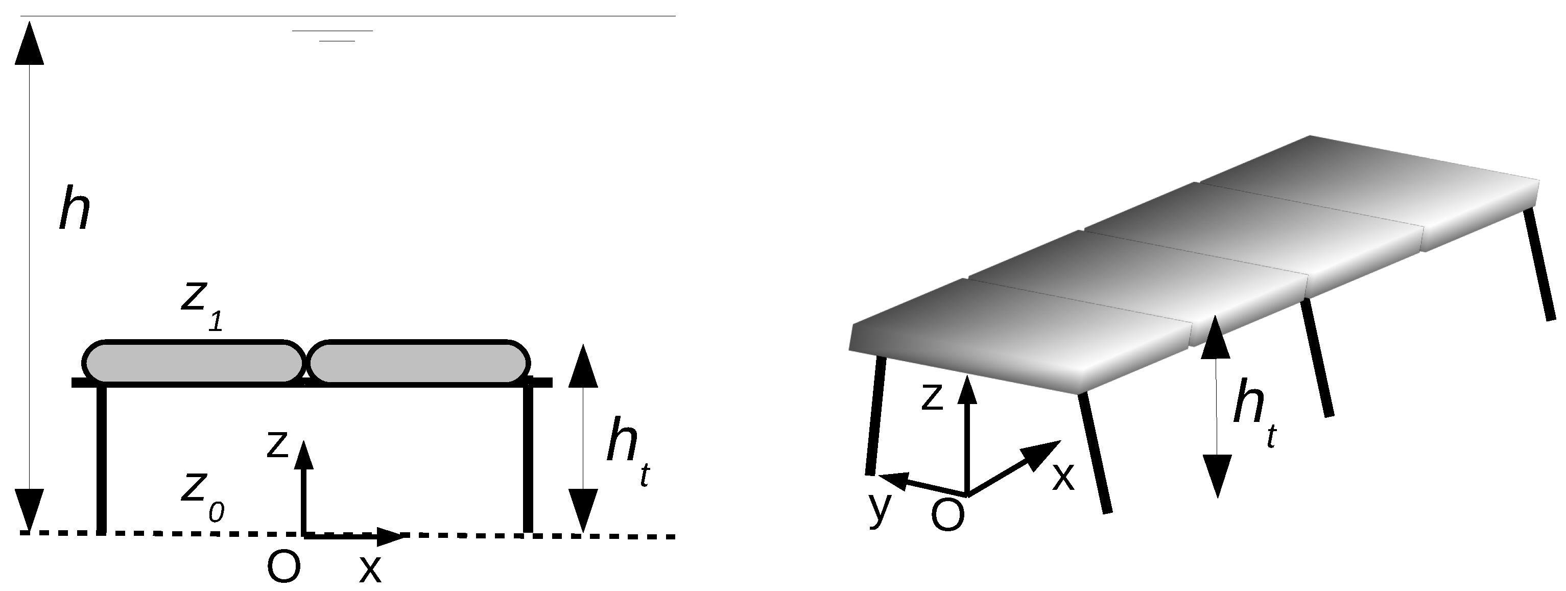
The modified version of the Chézy coefficient was established by considering two situations: (i) the case of unsubmerged structures where friction was driven by seabed roughness and drags of galvanised iron rods (supporting oyster tables) and (ii) the case of submerged structures which required considering the velocity profile above oyster tables and the flow interactions inside the oyster bags. The case of partially submerged structures (with a water level at the height of oyster bags) was not considered, thus assuming a negligible thickness of the bags, in comparison with the total water depth. Indeed, in this application, bag thickness was around for a spring tidal range over . Thus, the case of unsubmerged structures was obtained for a total water depth , with the height of the upper side of oyster tables, while the case of submerged structures was reached for . Figure 3 shows a schematic representation of oyster tables, with the main parameters considered for the formulations of the revised Chézy coefficient.
2.2.1. Unsubmerged Structures
For the case of unsubmerged tables (), the bottom shear stress was replaced by the total shear stress , expressed as the sum of the bed shear stress (Equation (1)) and the shear stress associated with iron rods :
with
D is the diameter of iron rods taken equal to [15], m is the number of rods per unit area, and is the drag coefficient of iron rods. The investigation considered oyster bags with a size of arranged in pairs on the different tables. Thus, a density of was retained. According to Meijer and Velzen [25], varies between 0.91 and 1.18 for steel bars. An average value of was retained in the present investigation, whereas such a value may differ from conditions characterised by an accumulation of algae around iron rods.
2.2.2. Submerged Structures
For the case of submerged structures (), differences appear with the previous situation, in relation to the establishment of the flow and associated boundary layers above and below the oyster tables. For a mean flow parallel to the oyster table direction (Ox in Figure 3), Kervella et al. [13] and Gaurier et al. [16] highlighted important areas characterised by a modification of the vertical velocity profile. These modifications were mainly associated with the development of three boundary layers: (i) an upper boundary layer above the table, (ii) a boundary layer in the lower part of the table, and (iii) another one next to the bottom. The two boundary layers below the oyster table interacted and merged, resulting in a maxima shifted towards the bottom. The characteristics of the flow were also impacted by the flow orientation, with respect to the oyster table direction. A minimum length of the table was, furthermore, required to stabilise the wake development and vertical profiles of horizontal velocity. As tables in the field were, most of the time, aligned with the main flow direction, this configuration was retained to propose a simple original parametrisation of the Chézy coefficient for the case of submerged structures.
As outlined in previous Section 2.2.1, the mathematical formulation of the friction coefficient requires expressing the bottom shear stress as a function of the depth-averaged velocity. However, for the case of submerged structures, such development is very complex to establish, as the vertical velocity profiles, below and over the oyster table, depend not only on the shear stress exerted at the bottom, but also on the shear stress exerted below and above the oyster structure. As exhibited by Gaurier et al. [16], the oyster bags may, furthermore, be considered as a porous media, thus impacting the classical logarithmic vertical velocity profile over the table. For these reasons, the effect of oyster farming structures on the flow was integrated as a sink term in the depth-averaged momentum equations of Telemac 2D, and this sink term was computed on the basis of the shear stress exerted over the oyster table, thus ignoring other contributions below the oyster structure. This development considered, therefore, that the major effects of submerged structures were associated with the friction of the upper part of oyster tables, and this was consistent with the simulations conducted by Kervella et al. [15] in the Mont-Saint-Michel bay. The associated friction coefficient was considered as a modified Chézy coefficient to remain consistent with the formulation for unsubmerged structures. The shear stress exerted over the oyster table was, thus, expressed as
with the shear velocity above the oyster table, the depth-averaged velocity for the upper part of the water column (over submerged tables), and the associated friction coefficient. The following vertical velocity profile was assumed over the oyster structure (for )
with the roughness parameter above the oyster table and the minimal velocity reached by the flow in the vicinity of the structure. In order to derive the friction coefficient , was assumed to be proportional to the depth-averaged part of the logarithmic velocity profile above the oyster table, thus resulting in the following relationship
with the coefficient retained for calibrating the minimal velocity.
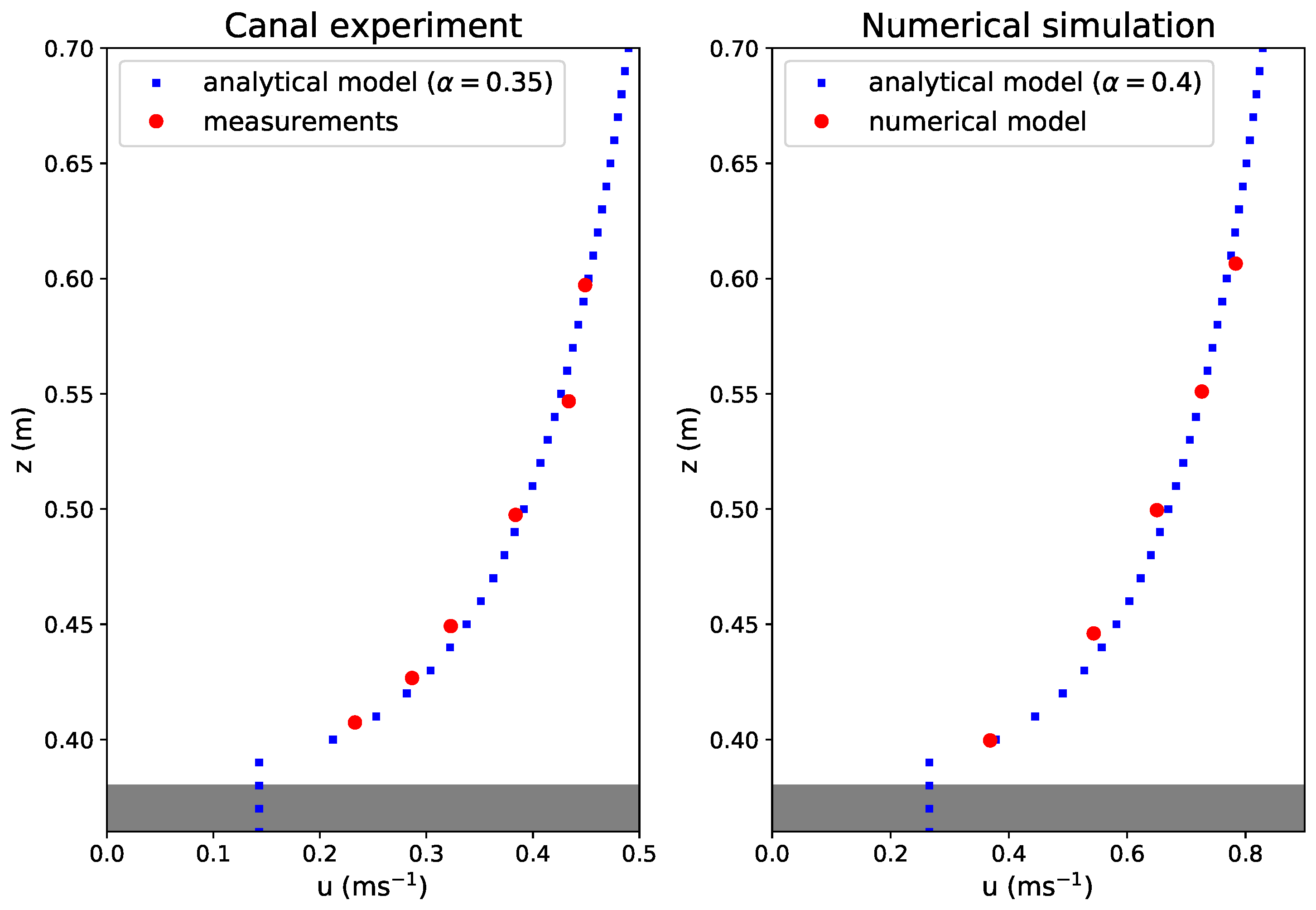
This analytical velocity profile (Equation (8)) was successively assessed against (i) the experimental measurements conducted by Kervella et al. [13] and (ii) the CFD simulation performed by Gaurier et al. [16] on a 1/2 scaled model of oyster table (Figure 4).
For these investigations, the height of oyster table was set to 0.35 m, with a width of 0.50 m and a total length of (i) 7.20 m for the physical laboratory experiment of Kervella et al. [13] and (ii) 72 m for the numerical modelling of Gaurier et al. [16]. The extended length of the oyster table in the numerical simulation allowed, thus, a full development of vertical wakes, which appeared restricted in the physical experiment. Velocity profiles were, furthermore, extracted for a configuration of current aligned with the table orientation in the median plane and at the downstream edge of oyster tables to guarantee a full development of vertical wakes. According to the dimension of the oyster tables in these two configurations, the velocity profiles were, therefore, extracted at a downstream length of 6.65 m for Kervella et al. [13] and 61.71 m for Gaurier et al. [16]. Resulted values of appeared a bit lower for the comparison with experimental data () than for the comparison with CFD predictions () (Figure 4). This difference may be associated with the partially developed velocity profile in the experimental measurements. For this reason, a coefficient was retained for the application in the Aber Wrac’h estuary.
Deriving the depth-averaged velocity from Equations (8) and (9) and integrating its formulation in Equation (7), the friction coefficient was expressed as
However, this coefficient can not be directly integrated to the numerical model, as it is associated with the depth-averaged velocity over the oyster table. Indeed, the modified Chézy coefficient , associated with the effect of the submerged tables on the flow, has to be expressed with respect to the depth-averaged velocity over the entire water column , this is in order to parametrise the sink term as a function of in the depth-averaged momentum equations. Thus, the shear stress exerted over the oyster table was expressed as a function of the coefficient
which resulted (from Equation (7)) in the following relationship between the two coefficients
The ratio between and was assumed to be the same without and with oyster tables (for a full development of boundary layers). This hypothesis was ascertained by comparing the ratio obtained from velocity profile measurements of Kervella et al. [13] () and predictions of Gaurier et al. [16] (), with the ratio derived from a theoretical logarithmic velocity profile without oyster tables (). This comparison exhibited reduced differences with values of 0.92 for and and 0.94 for . Thus, this ratio was considered constant without and with oyster tables, and the following relationship was finally derived for the modified Chézy coefficient with submerged structures
2.2.3. Synthesis
The revised formulations of the Chézy coefficient (Equations (6) and (13)) provide, therefore, a first estimation of the effects of oyster tables on the flow integrating, in particular, the height of the structure above the seabed and the possibility of a flow within the oyster bags. However, numerous approximations were adopted regarding the development of the boundary layer over the table and the estimation of the minimal velocity within the oyster bags or the conservation of the ratio with and without structures. These different assumptions and associated calibration coefficients were also established for an advanced growth of oyster, setting aside the reverse effects of oyster arrangement and size within bags. The Chézy coefficient here retained for submerged structures corresponds, furthermore, to the estimation of the bottom shear stress exerted over the oyster table setting aside the evolution of the velocity below the structure characterised by the development of two boundary layers (over the seabed and below the table). Thus, this friction coefficient has to be considered as a first approximation of the potential effects of oyster tables on the flow and can not be exploited to evaluate the sediment transport below the structure. It should also be noted that the thickness of the oyster bags were not considered in the estimation of the Chézy coefficient, thus neglecting the influence of the table on the velocity below the structure. This means that partially submerged structures () are integrated with Equation (6), setting aside the transition between non-submerged and submerged oyster tables. Nevertheless, in spite of these assumptions, the revised Chézy coefficient is a step towards a better approach of the variability of the friction coefficient associated with oyster tables for numerical simulations at the scale of macro-tidal estuarine environments. This is also an explicit formulation, which can be an alternative to classical parametrisations of depth-averaged models, based on a simple increase of the bottom roughness. This may finally serve as advanced three-dimensional investigations conducted at the scale of oyster structures.
2.3. Model Setup
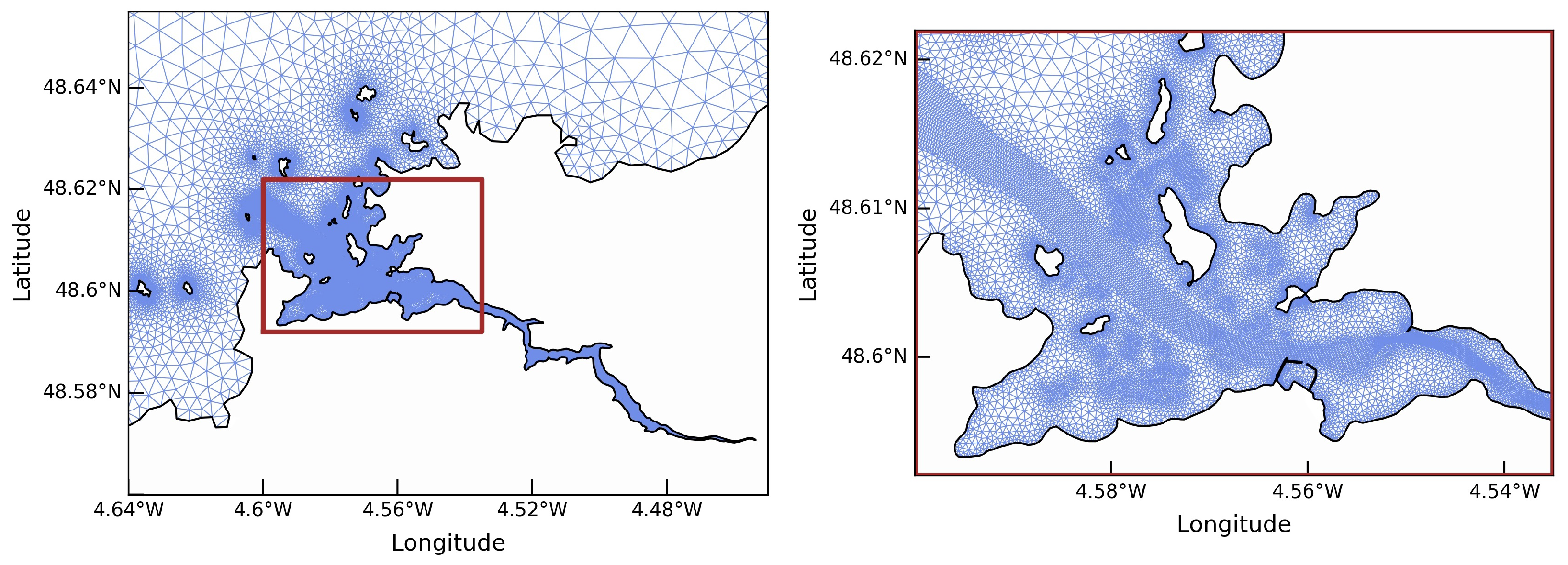
Telemac 2D was set up on an unstructured computational grid covering the Aber Wrac’h estuary and its outer extent. Thus, the seaward open boundary was located at the outer limit of northern Brittany to achieve suitable tidal forcings conditions (Figure 1). The river was also integrated to the computational domain, up to the tidal limit, to simulate the propagation of the tide in this environment (Figure 5).
The unstructured computational grid was composed of 25,014 nodes and 46,914 triangular elements with a spatial resolution of 3 km at offshore sea boundaries to less than 5 m within the upstream river limit. Particular attention was, furthermore, dedicated to the spatial resolution of the central channel and areas covered by oyster tables. The time step was set to 0.5 s. The bathymetry integrated (i) offshore, available data from the HOMONIM (“Historique, Observation, MOdélisation des NIveaux Marins”) project [26] and (ii), in the area of interest, data from the high-resolution coverage established during the Litto3D project [27]. It was also complemented by the local observations established as part of the present investigation by the Laboratory of Coastal Engineering and Environment (Cerema). According to Rollet et al. [19], most of seabed sediments was composed of mixed mud and sand in the estuary. The roughness parameter was, thus, set to an uniform value of , matching the observations for different bottom types compiled by Soulsby [24]. This value was consistent with the value of adopted by Robins et al. [22] to simulate the effects of climate change on solute transport within the Conwy estuary (UK). When considered, the effects of oyster structures on the tidal flow were included on areas covered by tables by (i) simply increasing the bottom roughness parameter to (the roughness parameter above the oyster tables) in the default Chézy formulation (Equation (2)) or (ii) including the modified version of the Chézy coefficient for unsubmerged and submerged configurations (Equations (6) and (13)). Thus, the default formulation considered by Kervella [15] to account for the large-scale effects of oyster tables on the flow was compared to the modified version to account for the effect of tidal range and the height of oyster tables. A value of was here retained. This value was consistent with the value determined by Kervella et al. [13] from the measurements of the vertical velocity profile in laboratory experiment and the value retained for the assessment of the analytical velocity profile (Figure 4). The ratio of roughness parameters between areas with and without oyster tables remained also consistent: a ratio of 20 for Kervella [15] against a ratio of 14 in the present investigation. The different parameters considered for the computation of the Chézy coefficients are shown in Table 1.
Following Guillou et al. [28], the model was finally driven by 13 major tidal harmonic components of the TPXO8-atlas database (, , , , , , , , , , , , and ) [29]. Coriolis effects were included, despite the potential negligible impacts on hydrodynamic conditions within the estuary. However, the effects of waves, wind, and atmospheric pressure were disregarded, restricting the investigation to the effects of oyster tables on the tidal flow. River discharges were, furthermore, neglected in accordance with local observations [30]. Three types of simulations were finally considered for investigating the effect of oyster tables on the tidal flow (Table 2).
3. Results and Discussion
3.1. Assessment of Model Predictions
3.1.1. Sea Surface Elevation
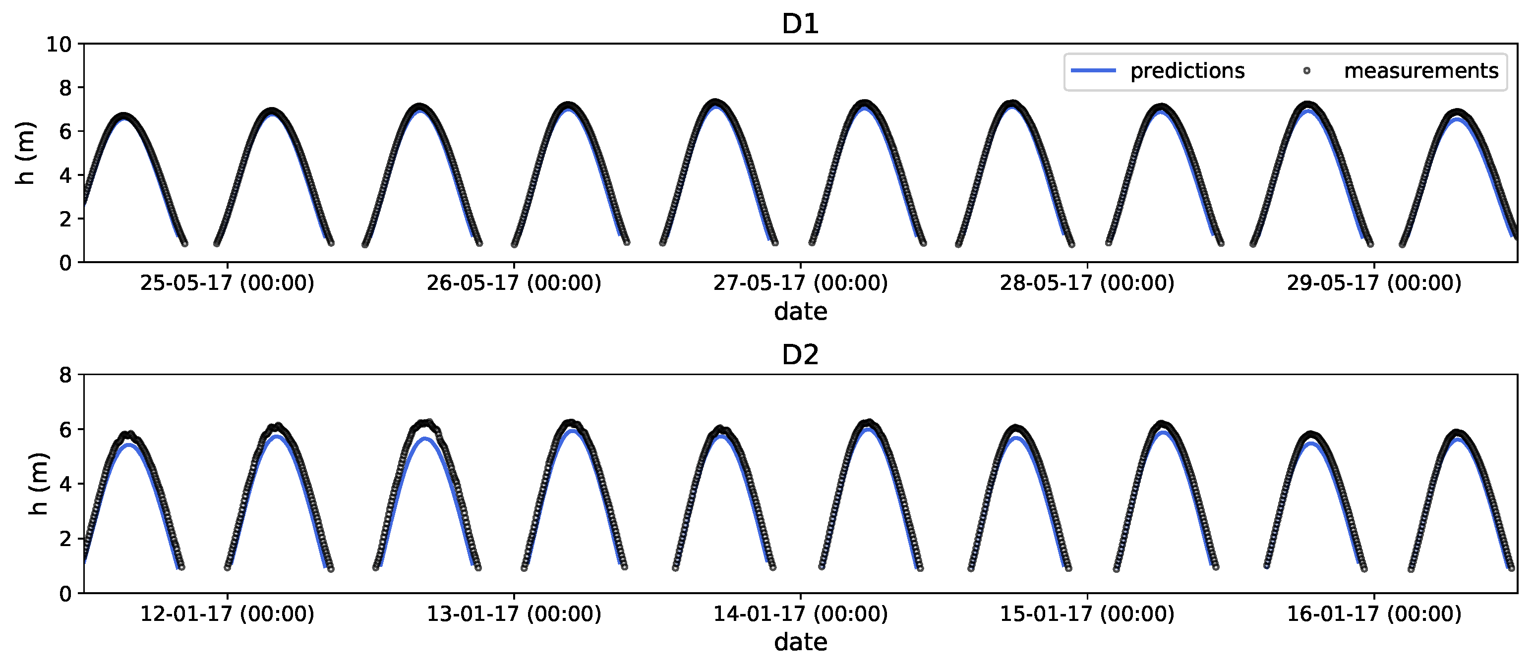
Predicted time series of the total water depth were first compared with measurements from pressure sensors at points D1 and D2 located in narrow passages between the islands and the landmass (Figure 2 and Figure 6). As reduced differences were obtained between the three numerical experiments (Table 2), the comparison was displayed for predictions , with the advanced parametrisation of the Chézy coefficient. Apart from the local differences seemingly being associated with the omission of pressure and wind effects in the numerical simulation, the predictions approached the observed tidal range with differences below and reduced time lag. Thus, this comparison confirmed the model’s performances in assessing the tide-induced variations of the total water depth over wetting–drying areas of the Aber Wrac’h estuary.
3.1.2. Current Velocity
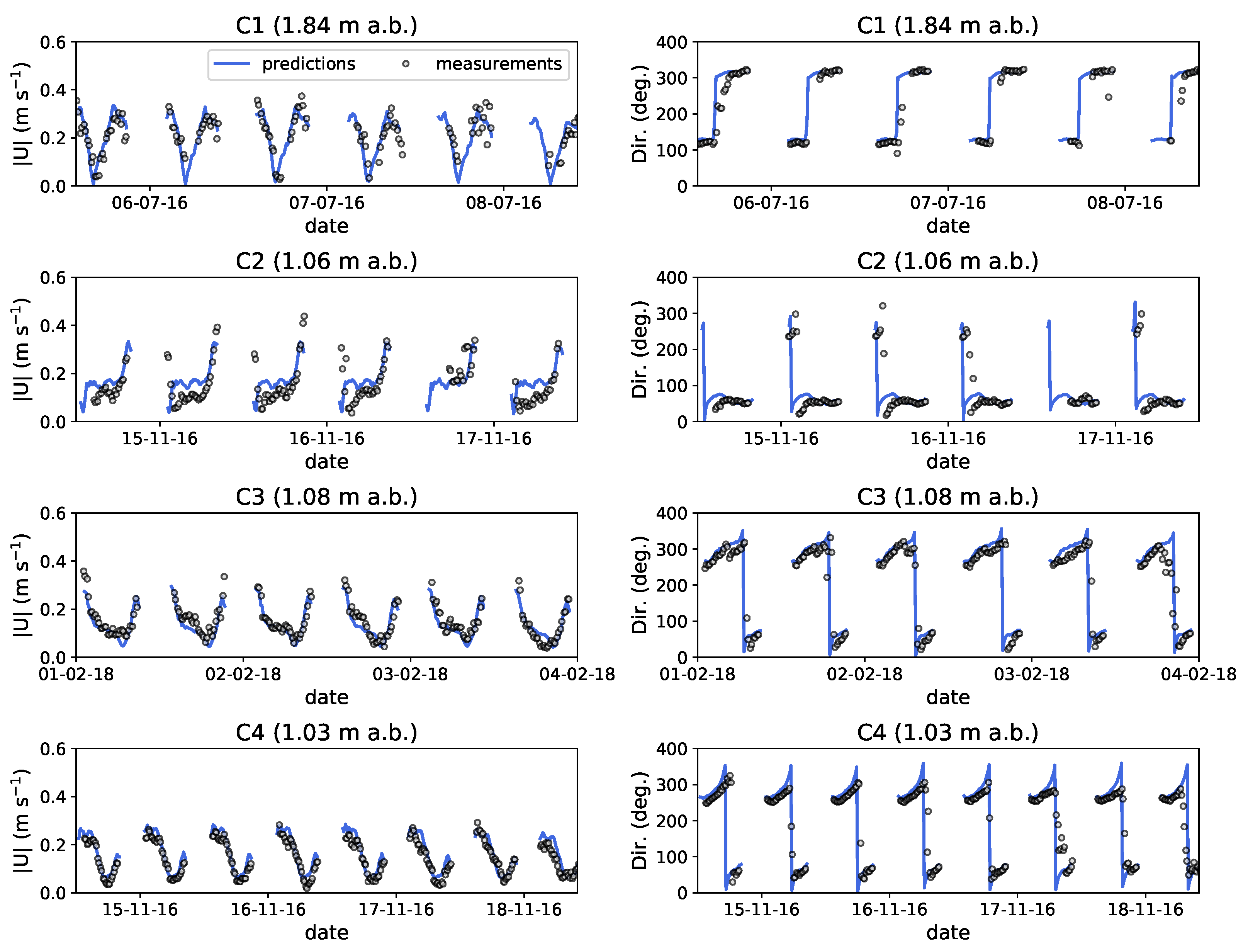
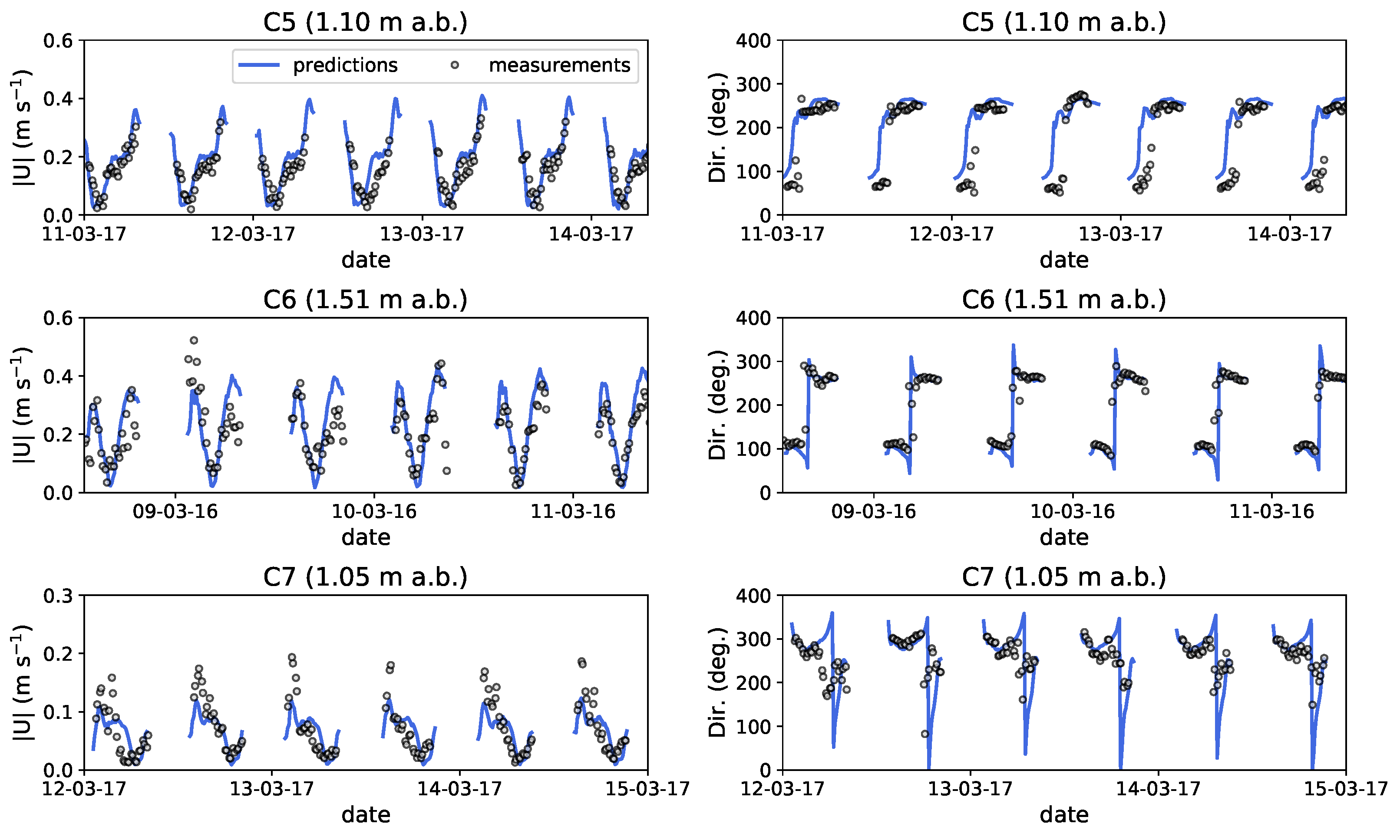
This evaluation was complemented by a comparison between predictions and in situ measurements of horizontal current magnitude and direction at seven locations disseminated in the western and eastern sides of the estuary (Figure 1). These measurements were acquired in spring tidal conditions over wetting–drying areas to facilitate the deployment and removal of the instrumentation systems. Thus, no recorded data was obtained at low tide. Measurements were conducted with upward looking acoustic doppler velocimeters and acquired at an acquisition rate of 8 Hz, every half hour, in 20-min records. Observed data were burst averaged to conduct the comparison with predictions. Predicted velocity magnitudes at the height of measurement points were extracted from the computed depth-averaged values assuming the vertical logarithmic velocity profiles. The numerical model in the configuration reproduced observed times series approaching the range of current magnitudes between (i) points, located in areas with restricted cross-sections or in the vicinity of an headland and characterised by peak magnitudes over (C1, C2, C5, and C6) and (ii) points located in very shallow waters at the bottom of bay and characterised by peak magnitudes below (C3, C4, and C7) (Figure 7 and Figure 8). Predictions also approached the abrupt changes of current direction observed between the ebb and flood at the different measurement locations. Slight improved estimations were obtained in the western side of the estuary than in its eastern side characterised by measurements points with lower water depths. The agreement between predictions and observations was, thus, particularly noticeable at points C3 and C4, located in the vicinity of oyster tables in the south-western side of the estuary.
3.2. Model Sensitivity to Bottom Friction Formulations
In this section, a first assessment of model sensitivity to bottom friction formulations (simple increase of roughness against new formulation) was conducted at the scale of the estuary by focusing on differences obtained in the predictions of tidal current magnitudes. The local effects of oyster tables on tidal circulation and sediment transport were investigated in next Section 3.3.
3.2.1. Global Tidal Circulation
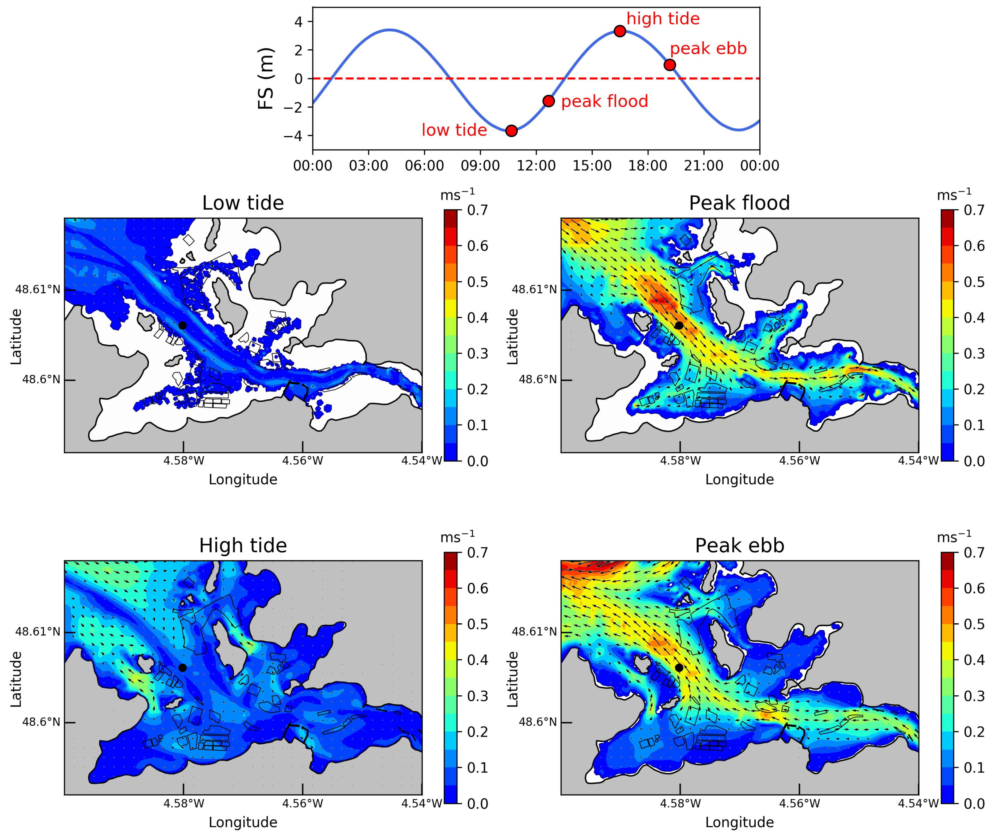
Model sensitivity to bottom friction formulations over oyster tables were investigated by relying on a first description of the tidal circulation at the scale of the estuary. Predictions were established during a mean spring tidal cycle in configuration (new formulation), thus providing a first overview of the different stages of tidal dynamics at times of low tide, peak flood, high tide, and peak ebb (Figure 9).
At low tide, the flow was restricted to the access channel, and the filling of the estuary was initiated with an increase of the tidal velocity up to values reaching at peak flood. Peak flood was characterised by an overflow of this access channel, leading to the filling of bays located on both sides. On these intertidal areas covered by oyster tables, tidal velocity magnitudes were restricted to values below . High tide showed naturally weak velocity magnitudes, with the strongest values exhibited in local straits between islands and the landmass. At peak ebb, the spatial distribution of tidal current magnitudes was quite similar to peak flood with maximum values predicted in the access channel. However, the emptying of the estuary was initiated in the northern part before impacting the two southern bays. These predictions confirmed also that tidal currents on both sides of the access channel were mainly orientated along the oyster tables, in agreement with the hypothesis formulated in Section 2.2.
3.2.2. Global Influence of Chézy Formulations on Tidal Current Magnitudes
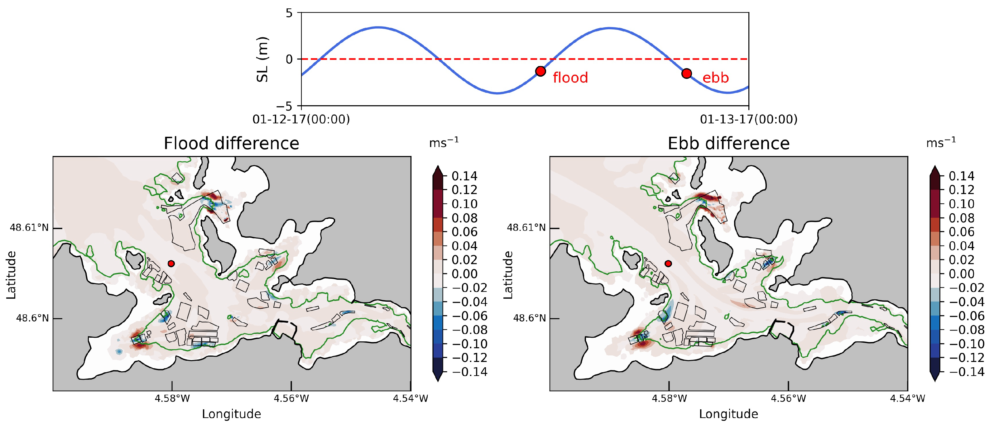
The sensitivity of model’s predictions to bottom friction formulations over oyster tables could not be assessed by relying on in situ observations. Indeed, slight differences were obtained in measurement locations between simulations with the two bottom friction formulations (simulations and , Table 2). Major changes concerned points C2, C3, and C4 in the south-western bay of the estuary, with a reduction of tidal current magnitudes with the new formulation (simulation ). The refined analysis of these differences required, therefore, a synoptic evaluation at the scale of the estuary. As a first overview of the global impact of oyster tables’ friction formulation, numerical predictions were, therefore, exploited to exhibit spatial differences in tidal current magnitudes during a mean spring tidal cycle, thus matching the synoptic description of the tidal circulation established in previous Section 3.2.1. Reduced modifications, restricted below , were obtained at times of high and low tides, in relation to the weak velocity magnitudes at these times of the tidal cycle (Figure 9). More important differences between the two friction formulations, reaching values over , were, however, exhibited at times of local peak flood and ebb near oyster tables, and these effects were mainly obtained for conditions of unsubmerged structures when the total water depth was below the height of tables ( with ) (Figure 10).
Indeed, for these conditions, the Chézy coefficient for the new formulation (Equation (6)) was mainly associated with the seabed bottom roughness (as iron rods had a minimal impact), and this contrasted with the increased roughness considered with the classical formulation. Thus, at these times of the tidal cycle, tidal currents in simulation (revised Chézy formulation) were very little influenced by the presence of oyster tables, whereas tidal currents in simulation (classical formulation) evolved, as if the oyster tables were submerged. Predictions were, therefore, impacted by the parametrisation retained for the friction associated with oyster tables with differences exceeding of current magnitudes in the vicinity of these structures at times of local peak velocities. This comparison also confirmed the interest of a refined investigation of the potential effects of oyster farming on the tidal circulation within estuaries characterised by macro-tidal regimes. Thus, these effects were investigated in the next section by relying on the new parametrisation (simulation ) and discussing these results with respect to differences obtained with the simple formulation (simulation ).
3.3. Effects of Oyster Tables
3.3.1. Tidal Current Magnitudes
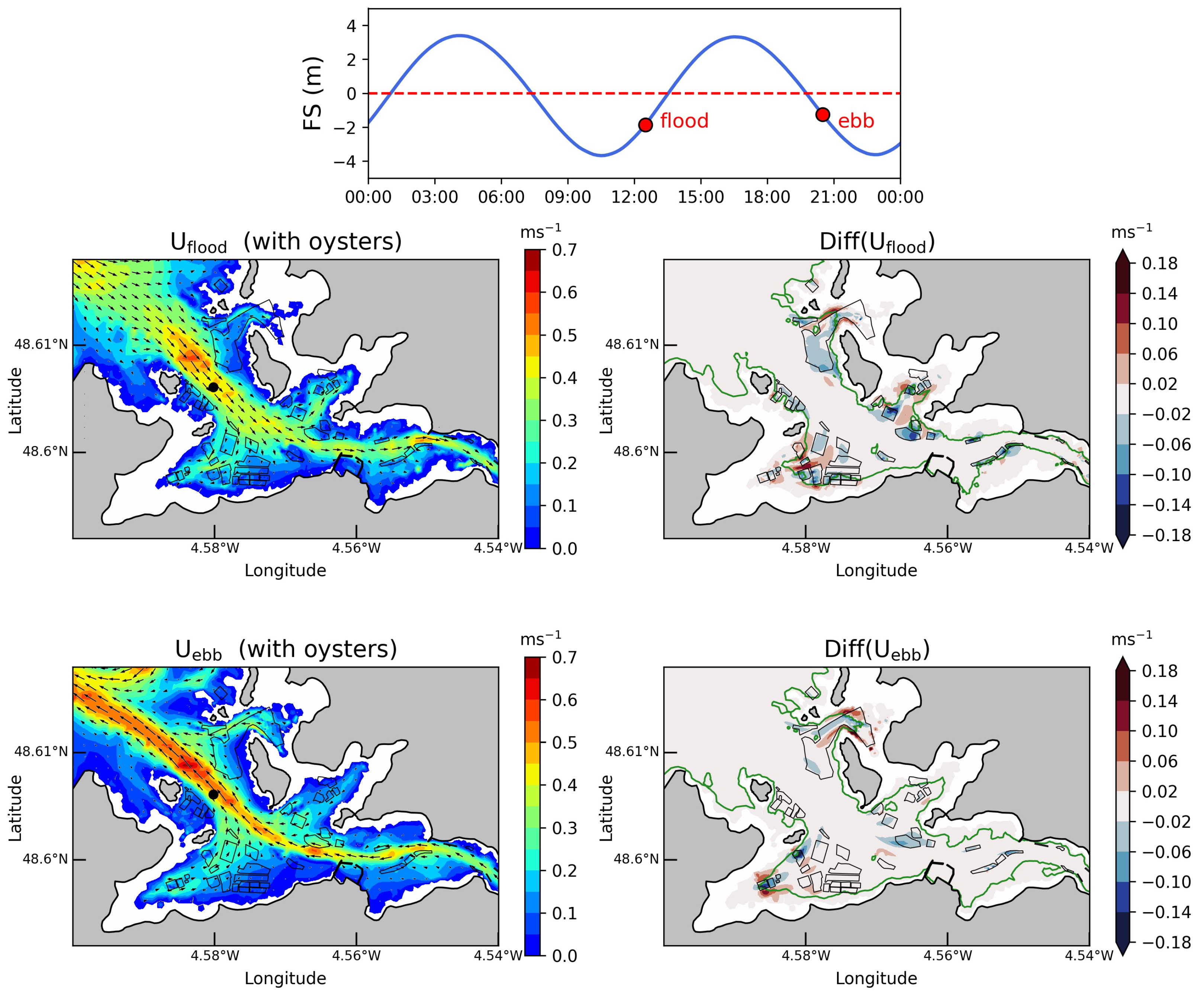
Modifications of tidal currents may impact the capacity of the environment to assimilate and disperse oyster wastes, resulting from biological filtering of suspended particulate matter [31]. Thus, as exhibited by Mitchell [32], increased currents will result in increased estuarine flushing, while reducing biodeposit accumulation with a series of effects on oxygen delivery to sediments and assimilation of farm wastes. Following the sensitivity study conducted on the Chézy parametrisation over oyster tables (Section 3.2.2), particular attention was, therefore, dedicated to modifications induced on tidal current magnitudes. The effects of oyster tables on the estuarine tidal circulation were assessed by comparing predictions from simulations (without oyster structures) and (with oyster structures and the revised formulation) (Table 2).
Maximum differences were obtained in the vicinity of oyster structures, and these differences were revealed at times of local peak flood and ebb for conditions of submerged structures with a water depth near the height of oyster tables (Figure 11).
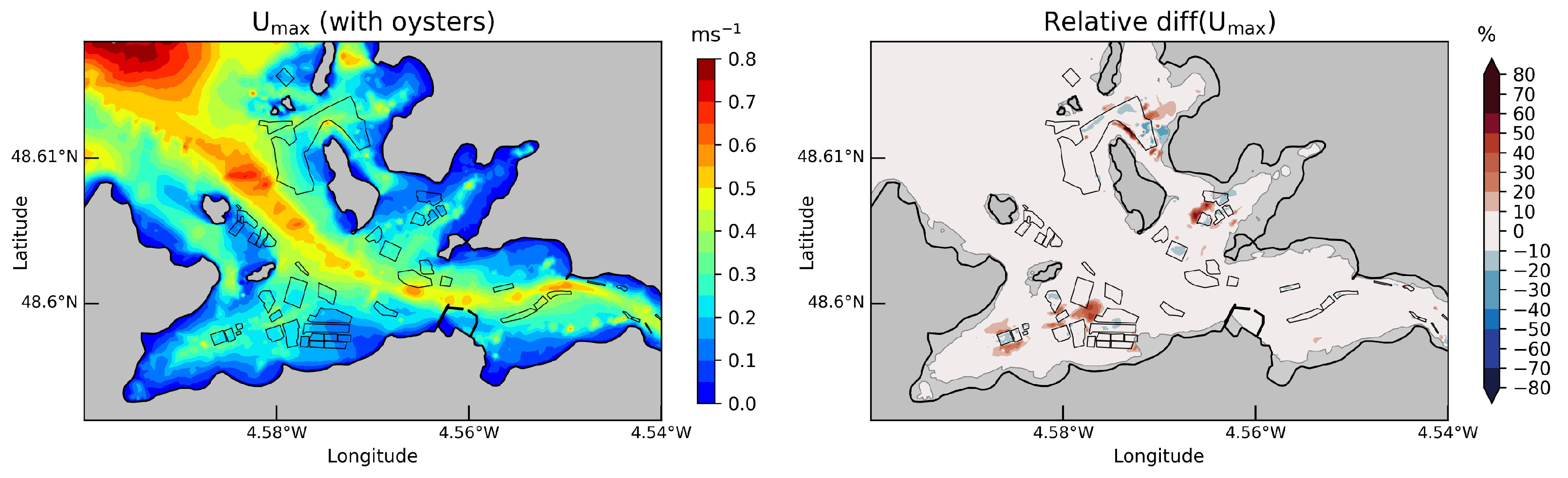
Indeed, these conditions exhibited the influence of the increased roughness of the upper part of oyster tables. For these conditions, predictions showed (i) a reduction of tidal current velocities over the areas covered by oyster tables, and both upstream and downstream, with (ii) an acceleration of the tidal flow on both sides of these areas characterised by reduced cross sections. In mean spring tidal conditions, maximum tidal currents were, thus, found to decrease by over oyster farming areas and increased of up to on both sides of these areas. These effects were particularly noticeable at the ends of north-eastern and south-western bays. Thus, in these intertidal areas characterised by reduced current velocity magnitudes, simulations exhibited an increase of maximum mean spring tidal currents exceeding on both sides of oyster farming areas, with a decrease between 10 and over these areas (Figure 12). Differences obtained with the default friction formulation over oyster tables (simulation ) also appeared in the vicinity of farming areas. However, matching the sensitivity study conducted in Section 3.2.2, these predictions resulted in a stronger decrease of maximum current velocities magnitude over the oyster tables (in relation to an increased bottom roughness in conditions of unsubmerged structures) associated with a lower increase on both sides of these structures.
Predicted changes of tidal current magnitudes induced by oyster tables suggested potential ecological effects, including especially local modifications of (i) biodeposition, (ii) the fouling of farm structures, and (iii) suspended particulate matter concentration. Thus, currents have to exceed a critical threshold to allow for dispersion and resuspension of seabed sediments and biodeposits [9]. For these reasons, particular attention was dedicated in the next sections to two parameters characterising these effects: (i) the velocity exceedance over a given threshold in areas covered by oyster tables and (ii) the sediment transport in the vicinity of these structures.
3.3.2. Velocities Exceedance
In practice, high current velocities are desirable in locations covered by oyster tables as a driver of increased food delivery, enhanced dispersal of biodeposits, and improved water quality [8,33]. Thus, well-flushed aquaculture sites are, most of the time, targeted to reduce these local benthic effects, in particular biodeposition and enrichment of seabed communities [34]. In order to investigate the local flushing characteristics of oyster farming areas and complement the study conducted on tidal current magnitudes, particular attention was dedicated to the fraction of time that the current magnitude was exceeding a given threshold over oyster farming areas. These characteristics were investigated during a mean spring tidal cycle for two threshold values, and , matching the range of velocities predicted over intertidal areas covered by oyster tables (Figure 13).
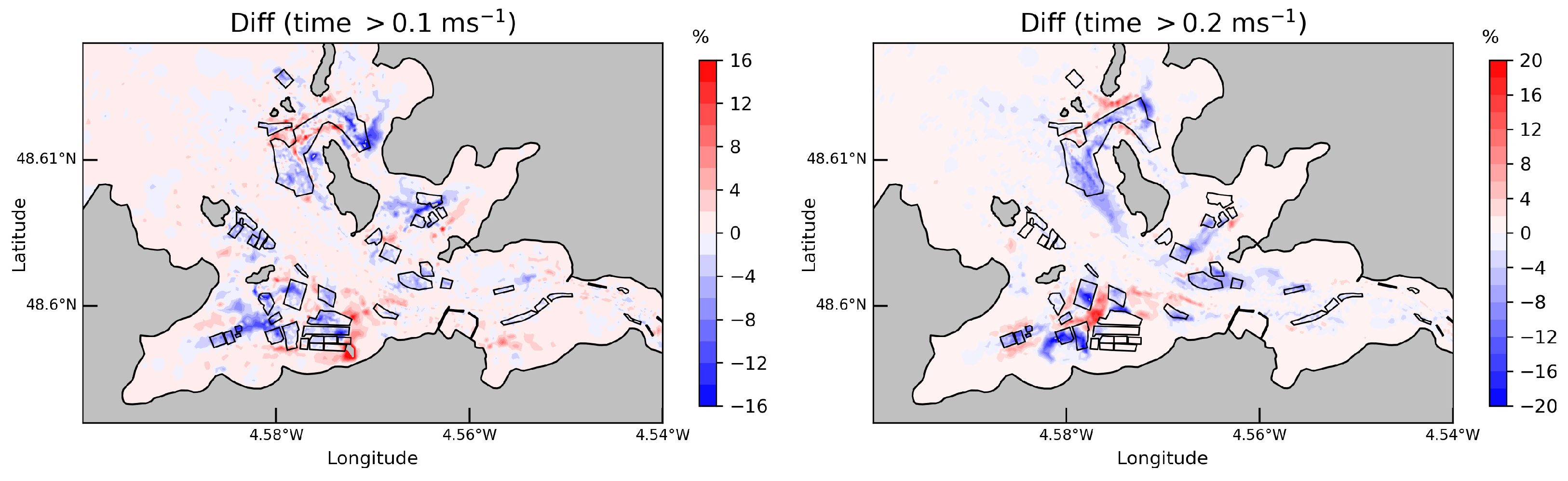
For the simulation without oyster tables, the current magnitude was initially exceeding for more than of the time over oyster farming areas bordering the access channel, and this percentage decreased below for tables located at the end of bays, especially in the south-western bay. Lower percentages were naturally obtained for a threshold value of . However, in both cases, simulations with the effects of oyster tables exhibited a decrease of time percentages by more than over oyster farming areas associated with a decrease of tidal current magnitude, and these effects were particularly noticeable in locations bordering the access channel between northern islands and the harbor of the estuary. The classical friction formulation (simulation ) resulted in increased differences over oyster tables with lower time percentages for velocities exceedance over these areas (Figure 14). These effects were also more pronounced for tables located at the end of bays. Indeed, as exhibited before, for simulation , these structures were considered as submerged throughout the tidal cycle, thus resulting in lower current velocities when the total water depth was below the height of tables. The approximation of constant submerged tables introduced with the classical formulation may, therefore, modify the spatial distributions of velocity exceedance over oyster farming areas.
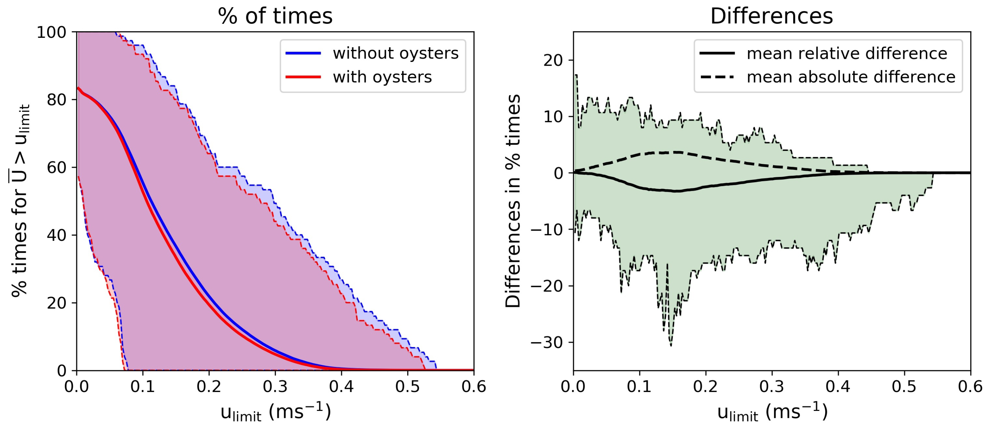
In order to investigate the overall effects of oyster tables, time percentages (i.e., fraction of the time during a mean spring tidal cycle) were finally (i) computed for different values in simulations and and (ii) averaged over areas covered by oyster tables (Figure 15).
Time percentages were characterised by a wide range of values (with variations over between the maximum and minimum values), as a result of the wide range of current magnitudes over areas covered by oyster tables in the vicinity of the access channel or at the end of bays. Averaged time percentages naturally decreased by increasing the threshold value . Major effects of oyster tables were, furthermore, obtained between values of 0.1 and . These effects were mainly noticeable for , with a difference between averaged time percentages of and a maximum difference of . This revealed that oyster tables may have locally a significant effect on the fraction of the time that the current remained over a given value. However, for the wide range of threshold values considered, these effects were very low, on average, at the scale of oyster farming areas.
3.3.3. Sediment Transport
Modifications induced by oyster tables on tidal current magnitudes may also impact the transport of sediment and particles (such as organic matter) in the vicinity of these structures. However, as described in Section 2.2, the modified formulation of the Chézy coefficient on submerged oyster tables was associated to the shear stress exerted over these structures. Thus, it was not possible to exploit depth-averaged velocities predicted over oyster tables for an approach of the bottom shear stress and the associated sediment transport below the tables. For these reasons, changes induced on sediment transport focused on locations outside of areas covered by oyster tables. A first preliminary evaluation was conducted by focusing on (i) the maximum diameters of seabed sediments liable to be moved in mean spring tidal conditions and (ii) changes induced by oyster structures. Maximum diameters were computed in two phases. The maximum bottom shear stress was first computed from the depth-averaged currents by assuming vertical logarithmic velocity profiles. The maximum diameters were then approached with the formulation of the critical shear stress proposed by Soulsby and Whitehouse [35].
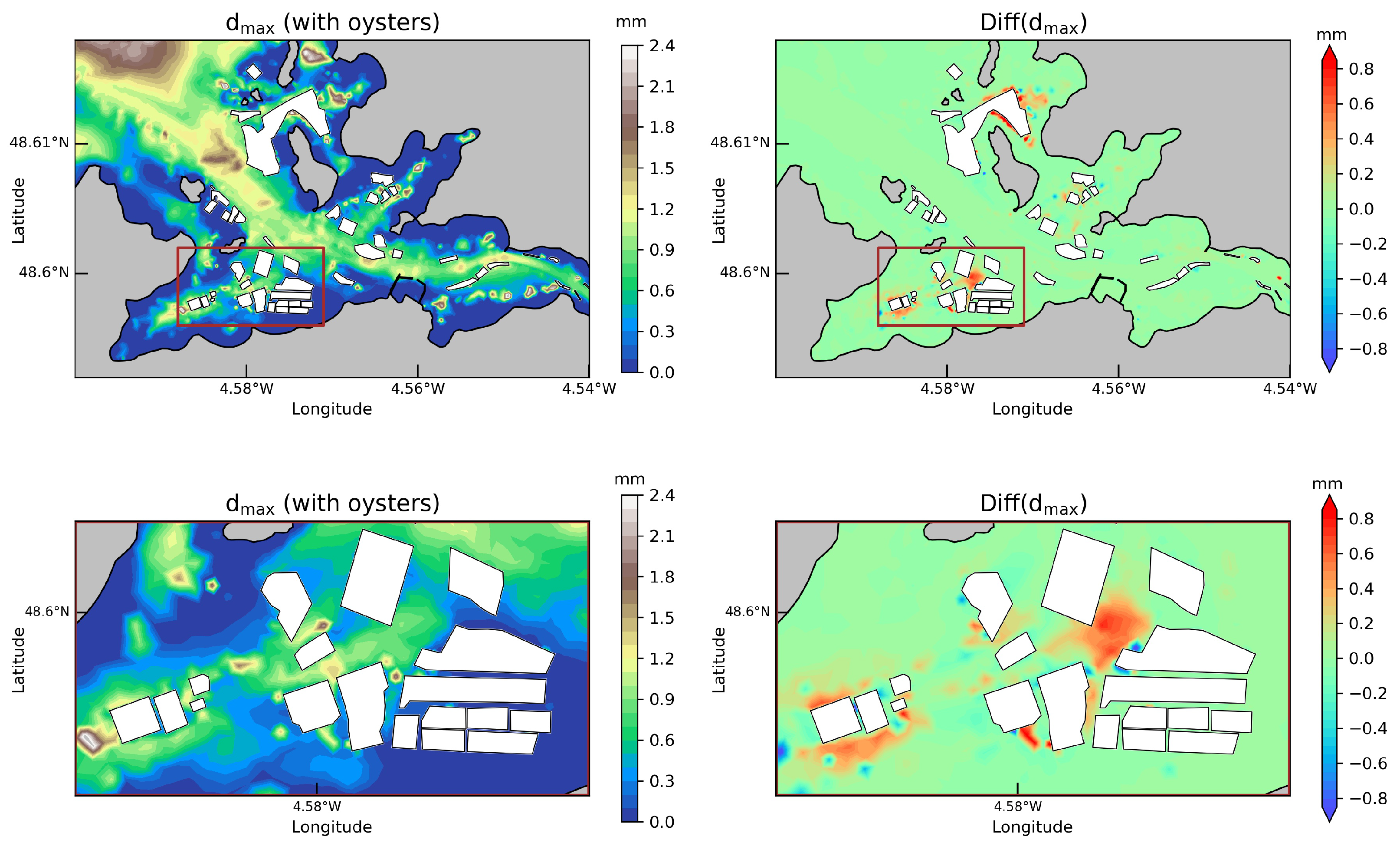
The resulted synoptic distribution revealed large areas in the vicinity of oyster structures where bed sediments with a diameter over 0.9 mm may be transported by tidal currents in mean spring condition (Figure 16).
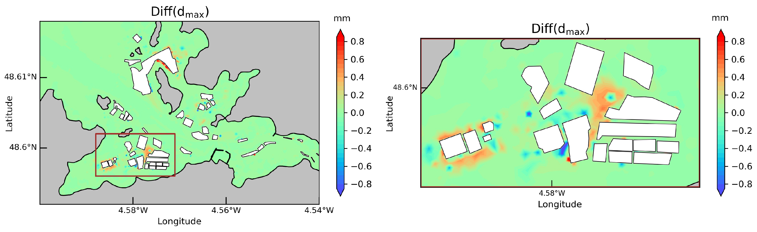
Thus, by increasing tidal current magnitude in these locations, oyster farming areas appeared responsible for the transport of this coarse sand. These effects were particularly noticeable in the south-western bay, where differences between simulations and exhibited variations of maximum sediments diameters up to 0.7 mm. The results obtained with the classical friction formulation (simulation ) naturally confirmed this tendency, resulting in increased maximum sediments diameters liable to be moved locally on both sides of oyster farming areas (Figure 17).
These predicted modifications of maximum sediments diameters liable to be moved during a spring tidal cycle, therefore, suggested an increased bedload and suspended sediment transport in the vicinity of oyster farming areas liable to impact the seabed morphology, but also the size and concentration of the depositional footprint, thus confirming a series of investigations dedicated to local changes in seabed topography and sedimentation (e.g., [14,36,37]). Further effects were also expected on local sediment enrichment by organic and fine particles resulting from biodeposition or sediment-water exchange in the vicinity of oyster tables [37]. Further investigations based on in situ observations may be required to assess these local predictions, and the results obtained appeared consistent with a series of studies which exhibited the local direct benthic effects of oyster cultivation restricted to tens of metres or less from farmed areas [9]. However, the results obtained required advanced investigations to approach, below tables, the evolution of the bottom shear stress in conditions of submerged structures that were liable to modify the sediment transport dynamics with potential sedimentation (e.g., [15]). Thus, the increased erosion identified on both sides of oyster farming areas may compete with the sediment transport below tables. Such advanced investigation may be based on local three-dimensional simulations of the vertical velocity profile over and below tables integrated the geometry of these structures (including the layout and spacing) at high spatial resolutions [16].
4. Conclusions
A depth-averaged tidal circulation model was exploited to investigate the hydrodynamic effects of elevated oyster cultivation within a small estuary of western Brittany (France). Particular attention was dedicated to the implementation of an original version of the Chézy coefficient, which was liable to approach the friction associated with these elevated structures during the different phases of the tidal cycle, thus integrating conditions of submerged and unsubmerged oyster tables. Numerical predictions were assessed against a series of in situ measurements of sea surface elevations and current velocities implemented during spring conditions in intertidal areas near oyster tables. The model was exploited to assess the sensitivity of numerical predictions to the Chézy parametrisation retained over oyster farming areas, comparing predictions obtained with this new formulation and the classical formulation based on a simple increase of the seabed roughness. Model predictions were, furthermore, exploited to assess the potential effects of oyster cultivation on tidal current magnitude, velocities exceedance over a given threshold and sediment transport. The main outcomes of the present investigation are as follows:
- The new Chézy formulation, here considered, relied on numerous approximations, including the alignment of current with table orientation, the development of vertical wakes and boundary layers, and the estimation of the minimal velocity within oyster bags. However, the associated analytical velocity profile (proposed here to express the Chézy coefficient) appeared consistent with experimental measurements and CFD predictions on a 1/2 scaled model. In preliminary studies, this revised formulation may, thus, be an interesting alternative to classical formulations based on a simple increase of the bottom friction, which neglected the conditions of submerged and unsubmerged structures in macro-tidal environments.
- Differences in the predictions of tidal current magnitudes were obtained between the two formulations of the Chézy coefficients considered in the vicinity of oyster structures at times of local peak flood and ebb. These effects were particularly noticeable for water depth near the height of oyster tables, thus exhibiting the limitation of the classical formulation to account for the temporal variations of the friction coefficient during the different phases of the tidal cycle.
- Predictions obtained with the revised formulation exhibited potential modifications of tidal velocities with (i) a reduction of current magnitudes over oyster farming areas and (ii) an acceleration of the tidal flow on both sides of these areas. Taking into account the reduced velocity magnitudes in intertidal areas, these modifications represented notable changes of current magnitudes with potential environmental effects.
- Thus, particular attention was dedicated to the fraction of time that the current magnitude was exceeding a given threshold value as an indicator of increased food delivery and water quality. However, despite the local high modifications, reduced changes of these velocities exceedance were obtained at the scale of areas covered by oyster tables.
- More important changes were finally exhibited on the surrounding sediment transport, in relation to the increased current magnitudes. Predictions suggested variations up to 0.7 mm of the maximum diameters of bed sediments liable to be moved in mean spring conditions. These effects were particularly noticeable in the south-western bay for structures bordering the access channel to the estuary. This suggested potential effects on seabed morphology and water quality.
The numerical results obtained promoted, therefore, a refined investigation of the Chézy coefficient associated with oyster cultivation. Such an explicit formulation of the Chézy coefficient was very convenient to encompass, at the scale of an estuary, the potential changes associated with the hydrodynamic modifications induced by oyster tables. However, the revised formulation and the depth-integrated approach considered require further improvements. Thus, among the different approximations adopted, particular attention may be dedicated to integrate the spacing between the rows of oyster tables and the establishment of a formulation liable to approach the bed shear stress and the associated sediment transport beneath tables. Indeed, for the case of submerged structures, the depth-averaged velocities were not representative of the vertical velocity profile below tables and, thus, of the bottom shear stress exerted on seabed sediments. Elevated oyster tables are, furthermore, aligned in rows with a spacing for the different operation required for this aquaculture, and this spacing may also impact the friction coefficient associated with oyster tables. These uncertainties introduced by the depth-integrated approach considered at the scale of the estuary, therefore, require advanced local three-dimensional investigations in the vicinity of structures, which may be conducted by relying on refined CFD simulations testing the different configurations of oyster tables arrangement. Such refined numerical approach of the interactions between oyster tables and the hydrodynamic flow will support the development of advanced simulations that are liable to encompass the transport of water particles at the scale of the estuary, thus investigating potential environmental impacts (with a focus on oyster farming), including harbor operations, macroalgal blooms, and the accidental release of pollutants or discharge of effluents and nutrients from terrestrial sources.
Funding
This research received no external funding.
Institutional Review Board Statement
Not applicable.
Informed Consent Statement
Not applicable.
Data Availability Statement
Not applicable.
Acknowledgments
A part of bathymetric data used here were provided by the French navy SHOM (“Service Hydrographique et Océanographique de la Marine”). Numerical simulations were conducted on HPC facilities DATARMOR of “Pôle de Calcul et de Données pour la Mer” (PCDM, https://pcdm.ifremer.fr, accessed on 1 January 2023). The author thanks François Gillet (Master’s degree, University of Western Brittany) and Yves Ponçon (ENSTA Paristech) for preliminary simulations of estuarine hydrodynamic conditions. The setup of instrumentation systems in the Aber Wrac’h estuary was conducted by Olivier Boucher and Antoine Douchin from Cerema research team. The present paper is a contribution to the research program INTERIMER (“INTEractions entre RIvière(s) et MER”) of the Laboratory of Coastal Engineering and Environment (Cerema, http://www.cerema.fr, accessed on 1 January 2023).
Conflicts of Interest
The author declares no conflict of interest.
References
- Gallardi, D. Effects of Bivalve Aquaculture on the Environment and Their Possible Mitigation: A Review. Fish. Aquac. J. 2014, 5, 8245. [Google Scholar] [CrossRef] [Green Version]
- O’Beirn, F.X.; Mckindsey, C.W.; Landry, T.; Costa-Pierce, B. Methods for Sustainable Shellfish Culture; Springer: Berlin/Heidelberg, Germany, 2012; pp. 9174–9196. [Google Scholar]
- FAO. The State of World Fisheries and Aquaculture—Meeting the Sustainable Development Goals; Food and Agriculture Organization of the United Nations: Rome, Italy, 2018. [Google Scholar]
- Yang, H.; Sturmer, L.; Baker, S. Molluscan Shellfish Aquaculture and Production. IFAS Extension, University of Florida, 2019. Available online: https://edis.ifas.ufl.edu/publication/FA191 (accessed on 1 January 2023).
- Solomon, O.; Ahmed, O. Ecological Consequences of Oysters Culture: A Review. Int. J. Fish. Aquat. Stud. 2016, 4, 01–06. [Google Scholar]
- DeFur, P.L.; Rader, D.N. Aquaculture in Estuaries: Feast or Famine? Estuaries 1995, 18, 2–9. [Google Scholar] [CrossRef]
- Read, P.; Fernandes, T. Management of environmental impacts of marine aquaculture in Europe. Aquaculture 2003, 226, 139–163. [Google Scholar] [CrossRef]
- Campbell, M.; Hall, S. Hydrodynamic effects on oyster aquaculture systems: A review. Rev. Aquac. 2019, 11, 896–906. [Google Scholar] [CrossRef]
- Forrest, B.M.; Keeley, N.B.; Hopkins, G.A.; Webb, S.C.; Clement, D.M. Bivalve aquaculture in estuaries: Review and synthesis of oyster cultivation effects. Aquaculture 2009, 298, 1–15. [Google Scholar] [CrossRef]
- Kirby, R. Sediments 2-oysters 0: The case histories of two legal disputes involving fine sediments and oysters. J. Coast. Res. 1994, 10, 466–487. [Google Scholar]
- Goslin, E. Marine Bivalve Molluscs, 2nd ed.; John Wiley & Sons: West Sussex, UK, 2015. [Google Scholar]
- Wildish, D.; Kristmanson, D. Benthic Suspension Feeders and Flow; Cambridge University Press: Cambridge, UK, 1997. [Google Scholar]
- Kervella, Y.; Germain, G.; Gaurier, B.; Facq, J.V.; Cayocca, F.; Lesueur, P. Experimental study of the near-field impact of an oyster table on the flow. Eur. J. Mech. B/Fluids 2010, 29, 32–42. [Google Scholar] [CrossRef] [Green Version]
- Nugues, M.; Kaiser, M.; Spencer, B.; Edwards, D. Benthic community changes associated with intertidal oyster cultivation. Aquac. Res. 1996, 27, 913–924. [Google Scholar] [CrossRef]
- Kervella, Y. Impact des Installations ostrÉicoles sur l’Hydrodynamique et la Dynamique Sédimentaire. Ph.D. Thesis, Université de Caen, Caen, France, 2010. [Google Scholar]
- Gaurier, B.; Germain, G.; Kervella, Y.; Davourie, J.; Cayocca, F.; Lesueur, P. Experimental and numerical characterization of an oyster farm impact on the flow. Eur. J. Mech. B/Fluids 2011, 30, 513–525. [Google Scholar] [CrossRef] [Green Version]
- Soletchnik, P.; Lambert, C.; Costil, K. Summer mortality of Crassostrea gigas (Thunberg) in relation to environmental rearing conditions. J. Shellfish. Res. 2005, 24, 197–207. [Google Scholar]
- SHOM. Courants de Marée et Hauteurs d’eau. La Manche de Dunkerque à Brest; Technical Report 564-UJA; Service Hydrographique et Océanographique de la Marine: Brest, France, 2000. [Google Scholar]
- Rollet, C.; Bonnot-Courtois, C.; Hamon, N.; Loarer, R. Réseau de Surveillance Benthique. Région Bretagne. Approche Sectorielle Intertidale. Cartographie des Habitats Benthiques, Secteur des Abers; Technical Report DYNECO/AG/11-06/CR; Ifremer: Brest, France, 2011; 47p. [Google Scholar]
- Hervouet, J.M. Hydrodynamics of Free Surface Flows, Modelling with the Finite Element Method; Cambridge University Press: Cambridge, UK, 2007; p. 311. [Google Scholar]
- EDF R&D. TELEMAC Modelling System—TELEMAC-3D Software—Release 6.2; Technical Report; EDF: Paris, France, 2013. [Google Scholar]
- Robins, P.; Lewis, M.; Simpson, J.; Howlett, E.; Malham, S. Future variability of solute transport in a macrotidal estuary. Estuarine Coast. Shelf Sci. 2014, 151, 88–99. [Google Scholar] [CrossRef] [Green Version]
- Guillou, N.; Thiébot, J. The impact of seabed rock roughness on tidal stream power extraction. Energy 2016, 112, 762–773. [Google Scholar] [CrossRef]
- Soulsby, R. The bottom boundary layer of shelf seas. In Physical Oceanography of Coastal and Shelf Seas; Johns, B.E., Ed.; Elsevier: Amsterdam, The Netherlands, 1983; pp. 189–266. [Google Scholar]
- Meijer, D.; Velzen, E.V. Prototype-scale flume experiments on hydraulic roughness of submerged vegetation. In Proceedings of the 28th International IAHR Conference, Paris, France, 25–28 August 1999. [Google Scholar]
- Jourdan, D.; Paradis, D.; Pasquet, A.; Michaud, H.; Gouillon, F.; Baraille, R.; Biscara, L.; Voineson, G.; Ohl, P. Le projet HOMONIM. Une contribution à l’amélioration de la prévision des submersions marines pour la Vigilance Vagues-Submersion. In Proceedings of the COCORISCO Conference, Brest, France, 3–4 July 2014. [Google Scholar]
- Louvart, L.; Grateau, C. The Litto3D project. In Proceedings of the Oceans 2005—Europe, Brest, France, 20–23 June 2005. [Google Scholar]
- Guillou, N.; Thiébot, J.; Chapalain, G. Turbines’ effects on water renewal within a marine tidal stream energy site. Energy 2019, 189, 116113. [Google Scholar] [CrossRef]
- Egbert, G.; Bennett, A.; Foreman, M. TOPEX/POSEIDON tides estimated using a global inverse model. J. Geophys. Res. 1994, 99, 24821–24852. [Google Scholar] [CrossRef] [Green Version]
- Merceron, M.; Gaffet, J.D. Température et Salinité dans l’Aber Benoît et l’Aber Wrac’h - été 1991—Rapport de Mesures; Technical Report; Ifremer: Plouzané, France, 1991. [Google Scholar]
- Souchu, P.; Vaquer, A.; Collos, Y.; Landrein, S.; Deslous-Paoli, J.M.; Bibent, B. Influence of shellfish farming activities on the biogeochemical composition of the water column in Thau Lagoon. Mar. Ecol. Prog. Ser. 2001, 218, 141–152. [Google Scholar] [CrossRef] [Green Version]
- Mitchell, I.M. In situ biodeposition rates of Pacific oysters (Crassostrea gigas) on a marine farm in Southern Tasmania (Australia). Aquaculture 2006, 257, 194–203. [Google Scholar] [CrossRef]
- Newell, C.; Hawkins, A.; Morris, K.; Richardson, J.; Davis, C.; Getchis, T. ShellGIS: A dynamic tool for shellfish farm site selection. J. World Aquac. Soc. 2013, 44, 50–53. [Google Scholar]
- Pearson, T.H.; Black, K.D. The environmental impact of marine fish cage culture. In Environmental Impacts of Aquaculture; Black, K.D.E., Ed.; Academic Press: Sheffield, UK, 2001; pp. 1–31. [Google Scholar]
- Soulsby, R.L.; Whitehouse, R.J.S.W. Threshold of sediment motion in coastal environments. In Proceedings of the Pacific Coasts and Ports ’97 Conference, Cristchurch, New Zealand, 7–11 September 1997; pp. 149–154. [Google Scholar]
- Everett, R.A.; Ruiz, G.M.; Carlton, J.T. Effects of oyster mariculture on submerged aquatic vegetation: An experimental test in a Pacific northwester estuary. Mar. Ecol. Prog. Ser. 1995, 125, 2205–2217. [Google Scholar] [CrossRef]
- Forrest, B.; Creese, R. Benthic impacts of intertidal oyster culture, with consideration of taxonomic sufficiency. Environ. Monit. Assess. 2006, 112, 159–176. [Google Scholar] [CrossRef] [PubMed]
Figure 1.
(a) Location of the study site in north-western European shelf seas. (b) Extent of the offshore computational domain in north western Brittany.
Figure 1.
(a) Location of the study site in north-western European shelf seas. (b) Extent of the offshore computational domain in north western Brittany.

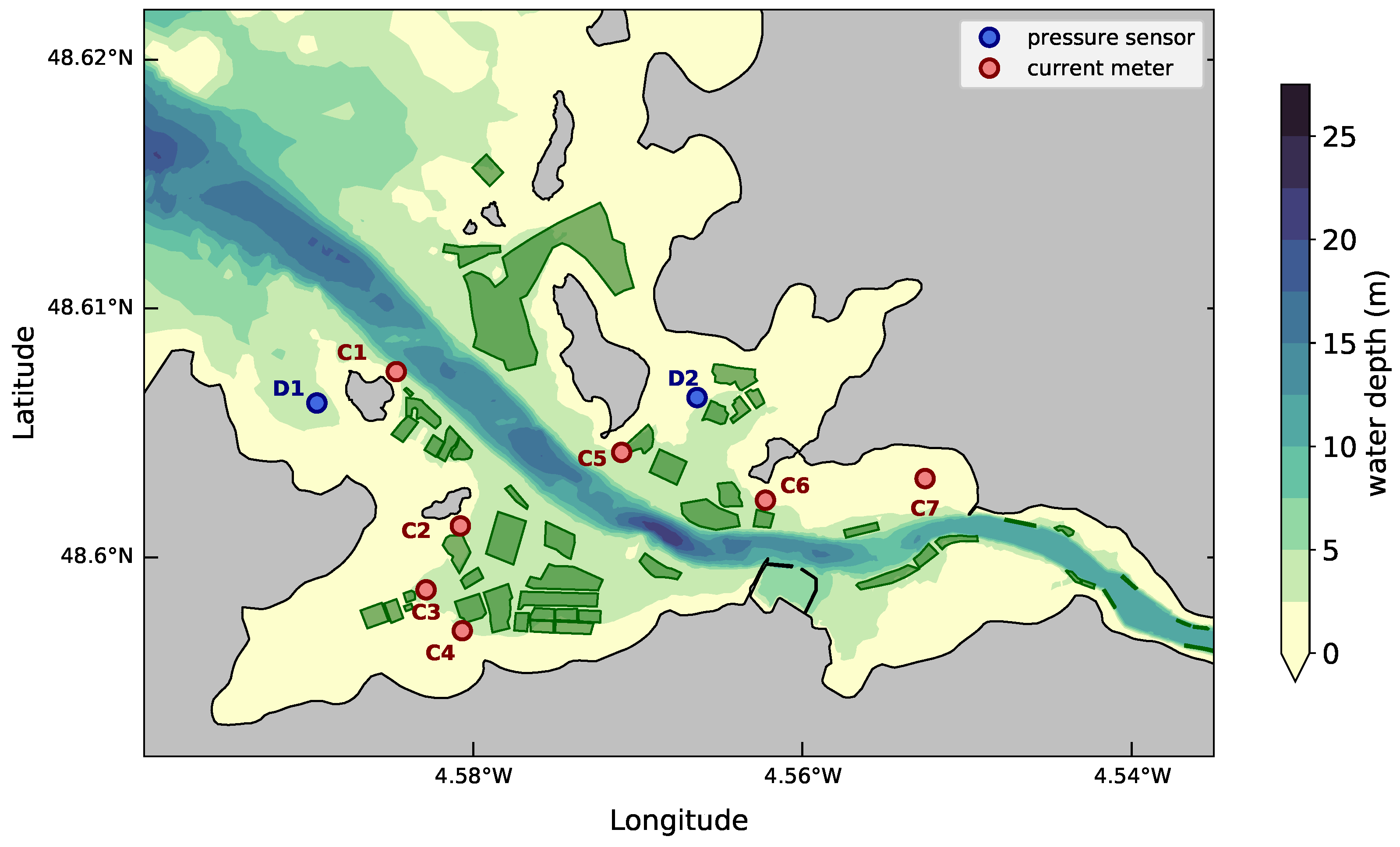
Figure 2.
Bathymetry of the Aber Wrac’h estuary located in western Brittany (France), with the locations of measurement points (pressure sensors and current meters). Green areas delimit the extents of oyster farming elevated structures within the estuary.
Figure 2.
Bathymetry of the Aber Wrac’h estuary located in western Brittany (France), with the locations of measurement points (pressure sensors and current meters). Green areas delimit the extents of oyster farming elevated structures within the estuary.

Figure 3.
Schematic representation of oyster tables.

Figure 4.
Vertical profiles of horizontal velocity over the oyster table obtained with the analytical model against velocity profiles (left) measured by Kervella et al. [13] and (right) computed by Gaurier et al. [16].

Figure 5.
Extents of the unstructured computational grid in the Aber Wrac’h estuary.

Figure 6.
Time series of observed and predicted total water depths with oyster tables (in configuration ) at points D1 ad D2.
Figure 6.
Time series of observed and predicted total water depths with oyster tables (in configuration ) at points D1 ad D2.

Figure 7.
Time series of observed and predicted (in configuration ) tidal current magnitude and direction (anticlockwise convention from the East) in the western part of the estuary at points C1, C2, C3, and C4 (a.b. for above the bed). Please note also that dates indicated correspond to midnight hour.

Figure 8.
Time series of observed and predicted (in configuration ) tidal current magnitude and direction (anticlockwise convention from the East) in the eastern part of the estuary at points C5, C6, and C7 (a.b. for above the bed). Please note also that dates indicated correspond to midnight hour.
Figure 8.
Time series of observed and predicted (in configuration ) tidal current magnitude and direction (anticlockwise convention from the East) in the eastern part of the estuary at points C5, C6, and C7 (a.b. for above the bed). Please note also that dates indicated correspond to midnight hour.

Figure 9.
Depth-averaged current velocities at low tide, peak flood, high tide, and peak ebb of a mean spring tide predicted in configuration . The top figure shows the time series of the free-surface elevation (with respect to mean water depth) in the access channel to the estuary (the location is indicated with a black circle on sub-figures). Time steps retained for the extraction of synoptic predictions are displayed with red circles on top figure. Black lines delimit the extents of areas covered by oyster tables.

Figure 10.
Differences in current magnitudes between simulations and at times of local peak flood and ebb near oyster tables during a mean spring tidal cycle. Positive values account for increased current magnitudes with the new parametrisation (), while negative values exhibit decreased current magnitudes. The green line corresponds to a total water depth of 0.8 m, the height of the upper side of oyster tables.

Figure 11.
(left) Depth-averaged currents during peak flood and ebb of a mean spring tide in configuration . (right) Differences in current magnitudes between simulations with () and without () the effects of oyster tables. Positive values account for an increase in current magnitude with oyster tables, while negative values exhibit a decrease in current magnitude. Top figure shows the time series of the free-surface elevation (with respect to mean water depth) in the access channel to the estuary (the location is indicated with a black circle on left figures). Time steps retained for the extraction of synoptic predictions are displayed with red circles on top figure. Black lines delimit the extents of oyster farming elevated structures, while green lines correspond to a total water depth of 0.8 m, the height of the upper side of oyster tables.

Figure 12.
(left) Maximum magnitudes of depth-averaged currents in mean spring tidal conditions predicted with oyster tables (). (right) Relative differences in current magnitudes between simulations with () and without () the effects of oyster tables. Differences are shown for current magnitude over . Positive values account for an increase in current magnitude with oyster tables, while negative values exhibit a decrease in current magnitude.

Figure 13.
(left) Percentage of times for and during a mean spring tidal cycle in conditions without oyster tables (). (right) Differences predicted with oyster tables (between simulations and ).
Figure 13.
(left) Percentage of times for and during a mean spring tidal cycle in conditions without oyster tables (). (right) Differences predicted with oyster tables (between simulations and ).

Figure 14.
Differences in percentage of times for and during a mean spring tidal cycle between simulations and .
Figure 14.
Differences in percentage of times for and during a mean spring tidal cycle between simulations and .

Figure 15.
(left) (filled line) Evolution of the fraction of the time during a mean spring tidal cycle, averaged over areas covered by oyster tables in simulations (without oysters) and (with oysters). The upper and lower lines show the maximum and minimum time percentages reached over oyster farming areas for a given value of , respectively. (right) Mean relative and absolute differences (–) between time percentages averaged over areas covered by oyster tables. Thus, the black line on this sub-figure shows the difference between filled lines on the left sub-figure. The upper and lower lines show the maximum and minimum differences in time percentages over oyster farming areas for a given value of . Negative values show, therefore, a decrease of times percentages with oysters while positive values accounts for an increase.

Figure 16.
(top left) Maximum diameters of bed sediments liable to be moved in mean spring tidal conditions (simulation with oyster tables ). (top right) Differences with respect to the situation without oyster tables (–). The red box in top sub-figures shows the area considered for a detailed view in bottom sub-figures.

Figure 17.
Differences in maximum diameters of bed sediments liable to be moved in mean spring tidal conditions between simulations and .
Figure 17.
Differences in maximum diameters of bed sediments liable to be moved in mean spring tidal conditions between simulations and .


Table 1.
Values retained for parameters considered in the computation of the modified Chézy coefficients.
Table 1.
Values retained for parameters considered in the computation of the modified Chézy coefficients.
| Parameters | Definition | Value |
|---|---|---|
| height of the upper side of oyster bags | 0.8 m | |
| m | number of rods per unit area | |
| D | diameter of iron rods | 0.016 m |
| drag coefficient of iron rods | 1.0 | |
| coefficient for calibrating | 0.4 | |
| seabed bottom roughness | ||
| roughness of upper part of oyster tables |
Disclaimer/Publisher’s Note: The statements, opinions and data contained in all publications are solely those of the individual author(s) and contributor(s) and not of MDPI and/or the editor(s). MDPI and/or the editor(s) disclaim responsibility for any injury to people or property resulting from any ideas, methods, instructions or products referred to in the content. |
© 2023 by the author. Licensee MDPI, Basel, Switzerland. This article is an open access article distributed under the terms and conditions of the Creative Commons Attribution (CC BY) license (https://creativecommons.org/licenses/by/4.0/).
Share and Cite
MDPI and ACS Style
Guillou, N. Modelling the Effects of Oyster Tables on Estuarine Tidal Flow. Coasts 2023, 3, 2-23. https://doi.org/10.3390/coasts3010002
AMA Style
Guillou N. Modelling the Effects of Oyster Tables on Estuarine Tidal Flow. Coasts. 2023; 3(1):2-23. https://doi.org/10.3390/coasts3010002
Chicago/Turabian StyleGuillou, Nicolas. 2023. "Modelling the Effects of Oyster Tables on Estuarine Tidal Flow" Coasts 3, no. 1: 2-23. https://doi.org/10.3390/coasts3010002