
Documenting the Evolution of a Southern California Coastal Lagoon during the Late Holocene


Abstract
:1. Introduction
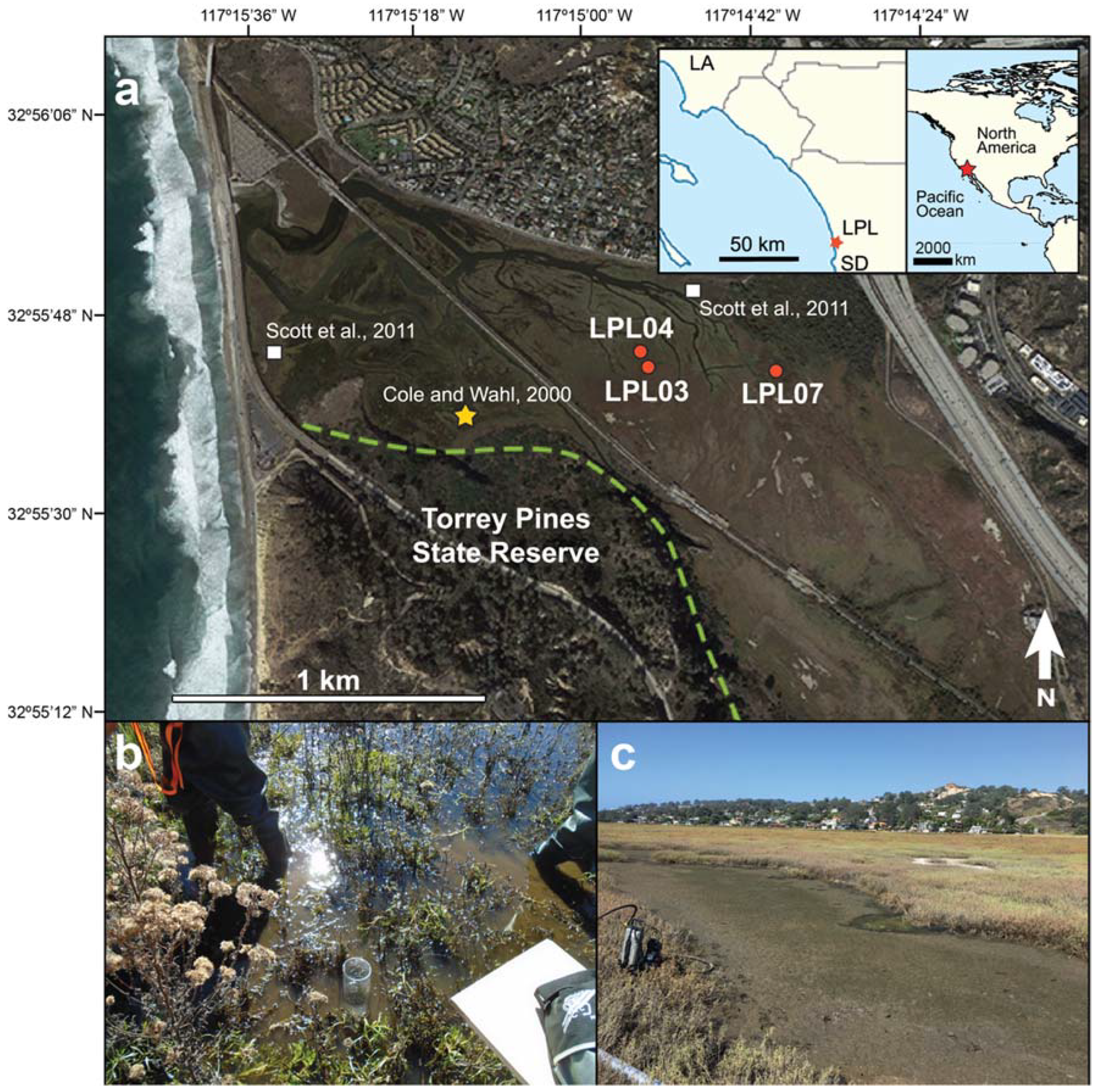
2. Study Area
3. Materials and Methods
3.1. Core Collection and Descriptions
3.2. Grain Size Analyses
3.3. Loss-on-Ignition
3.4. Shell Analyses
3.5. Radiocarbon Dating
4. Results
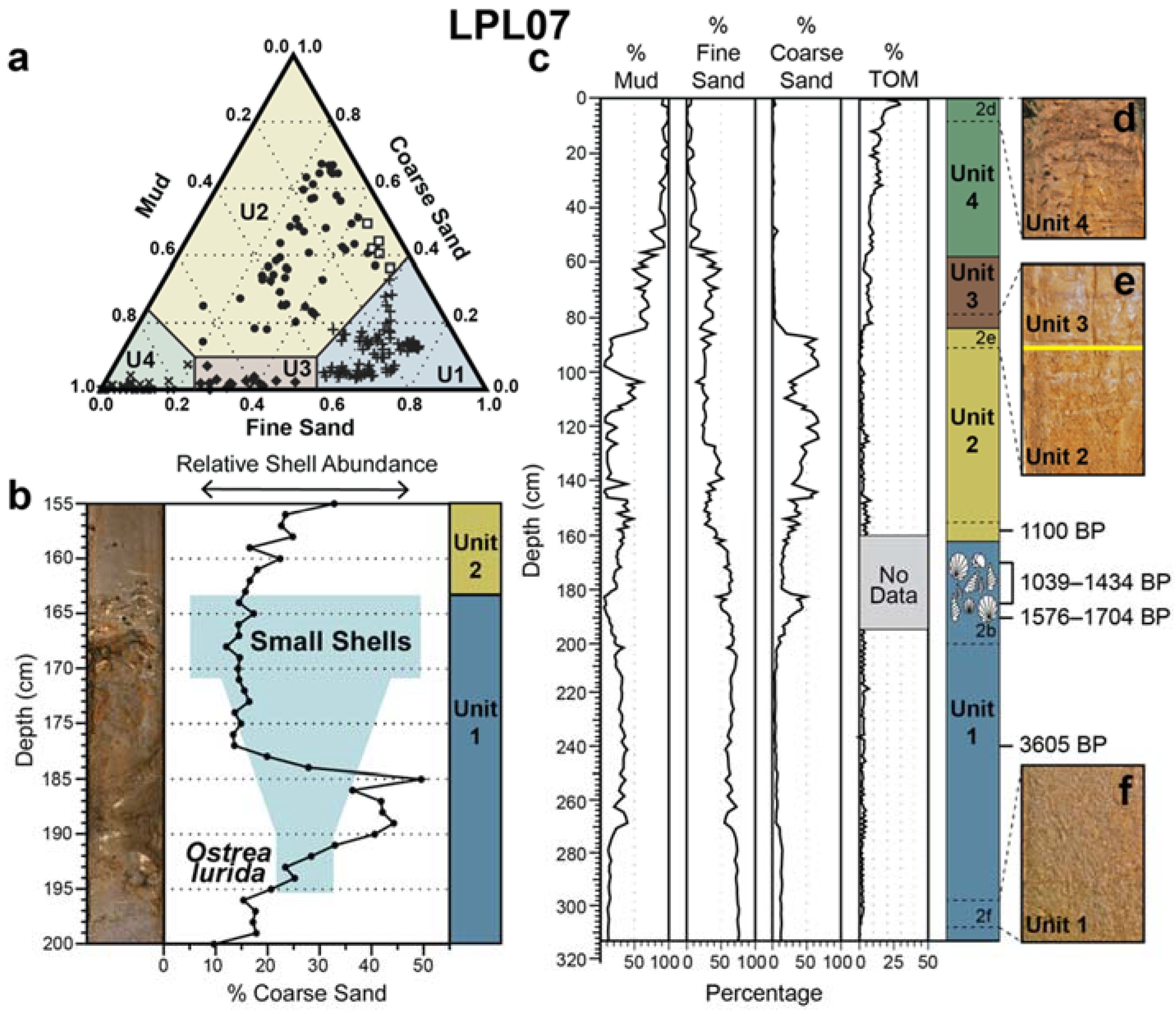
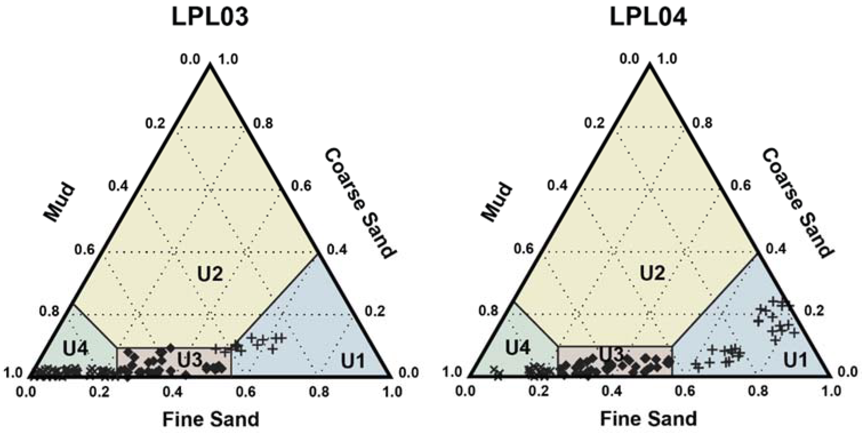
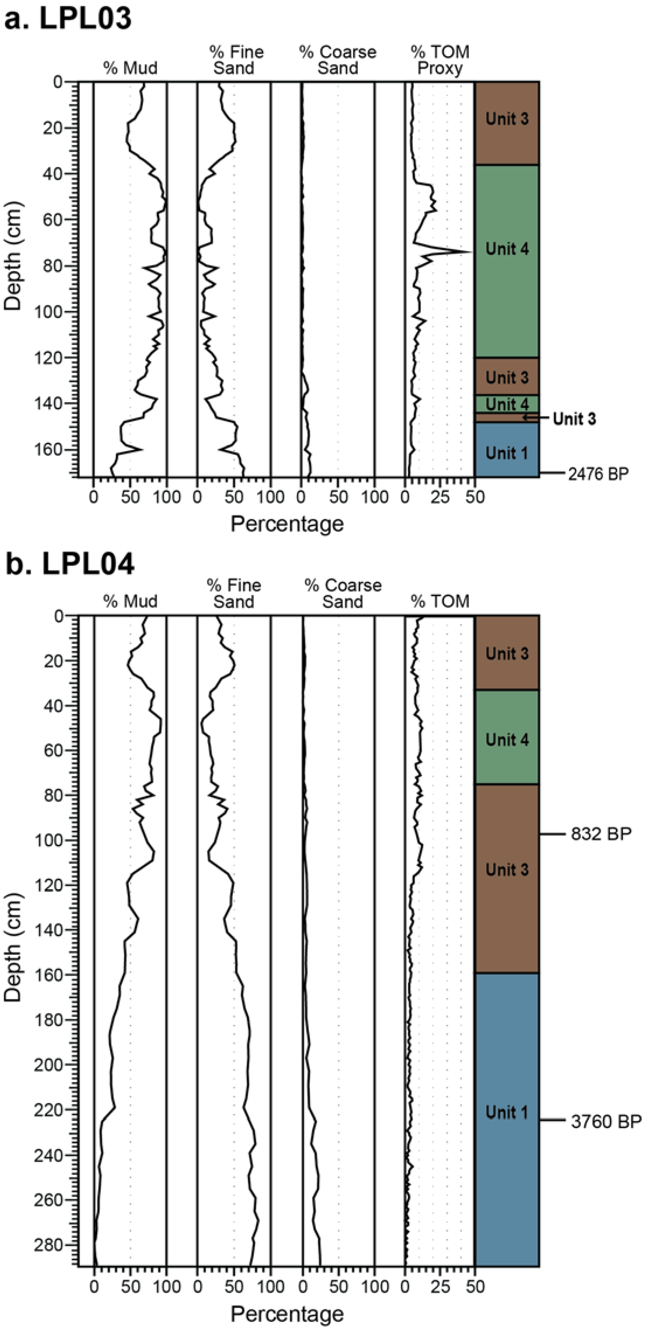
4.1. Core Description and Grain Size
4.2. Loss-on-Ignition
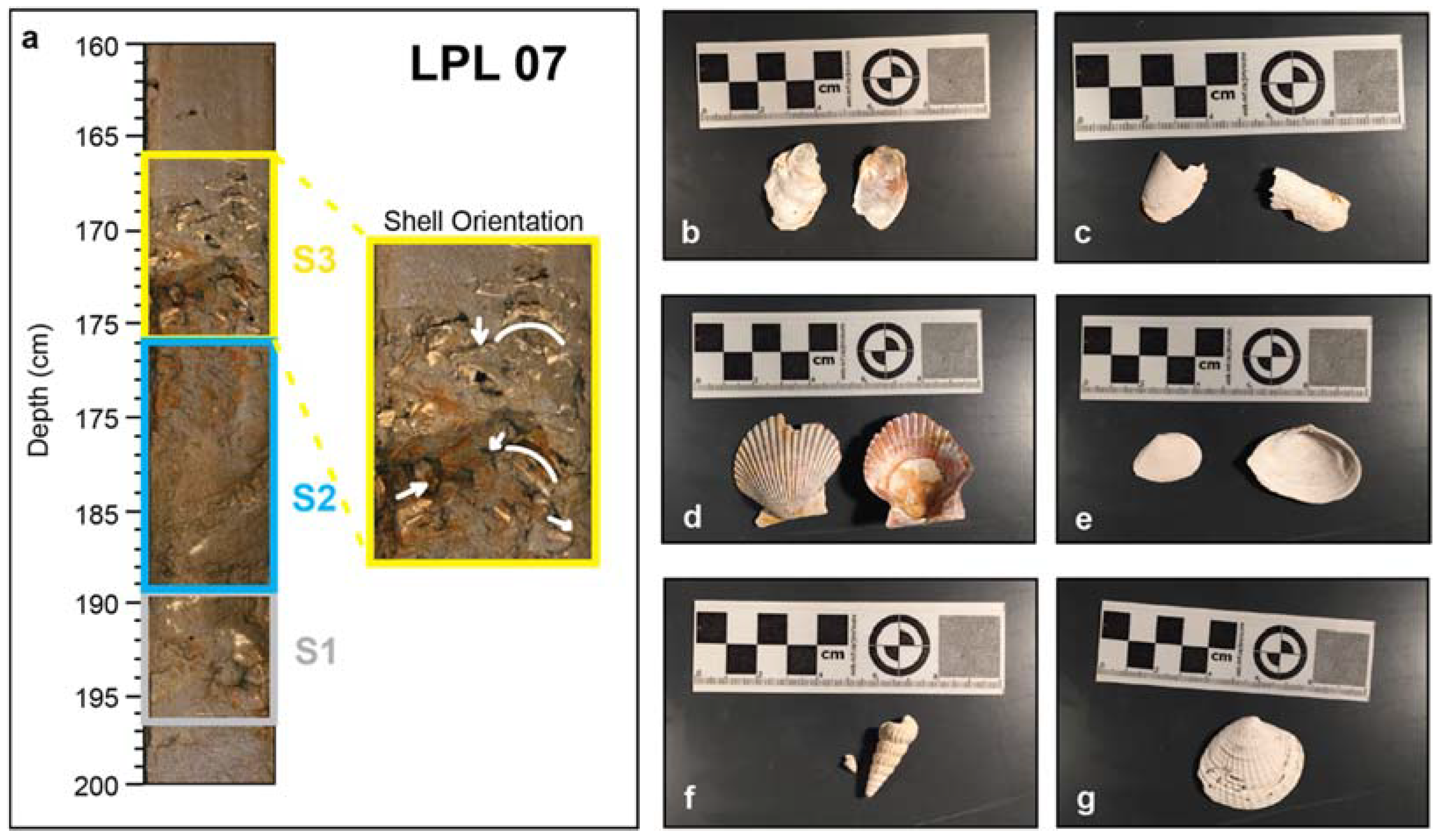
4.3. Shell Analysis
4.4. Radiocarbon Dating
5. Discussion
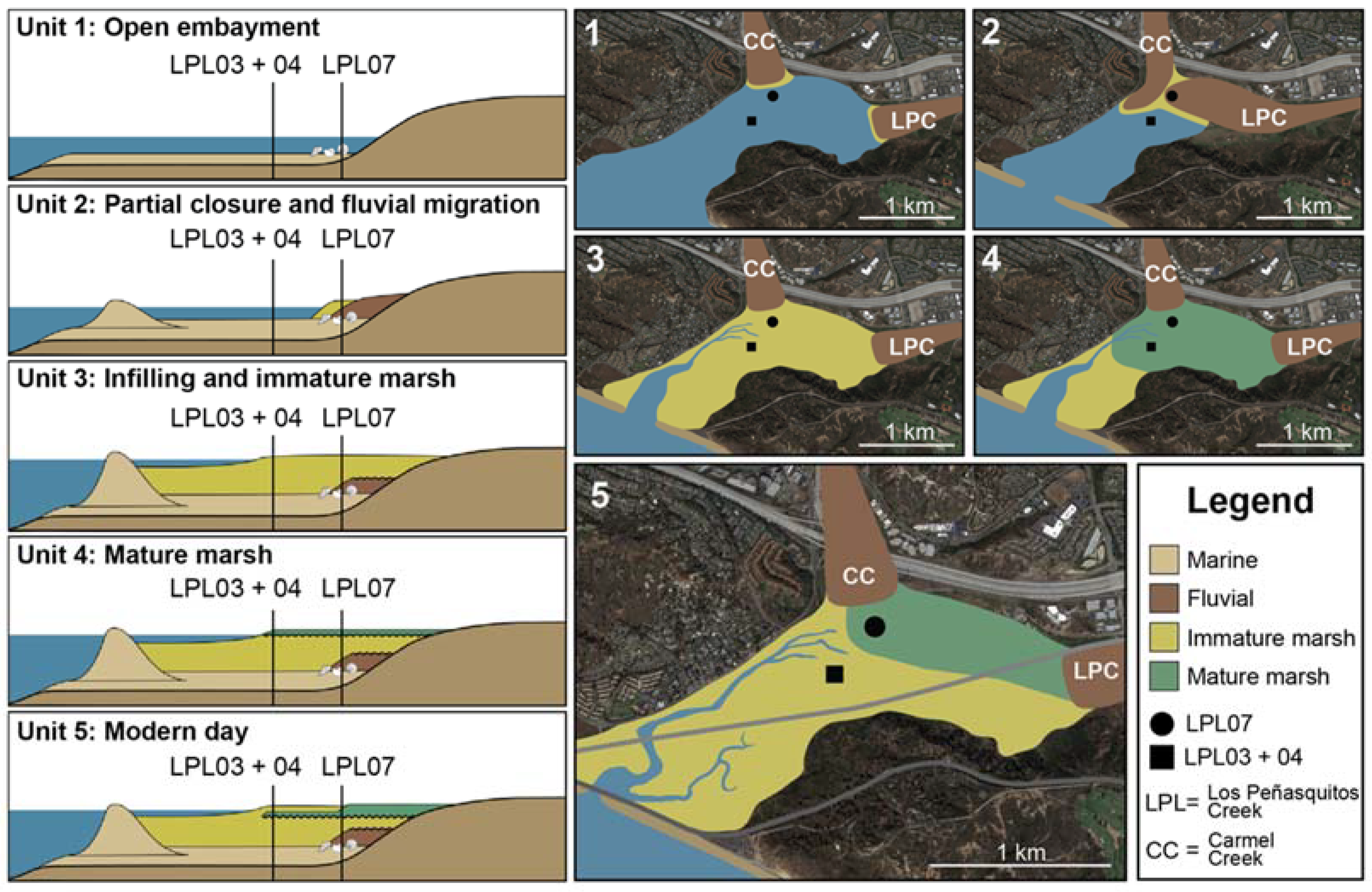
5.1. Sedimentary Facies
5.2. Shell Hash Interpretations
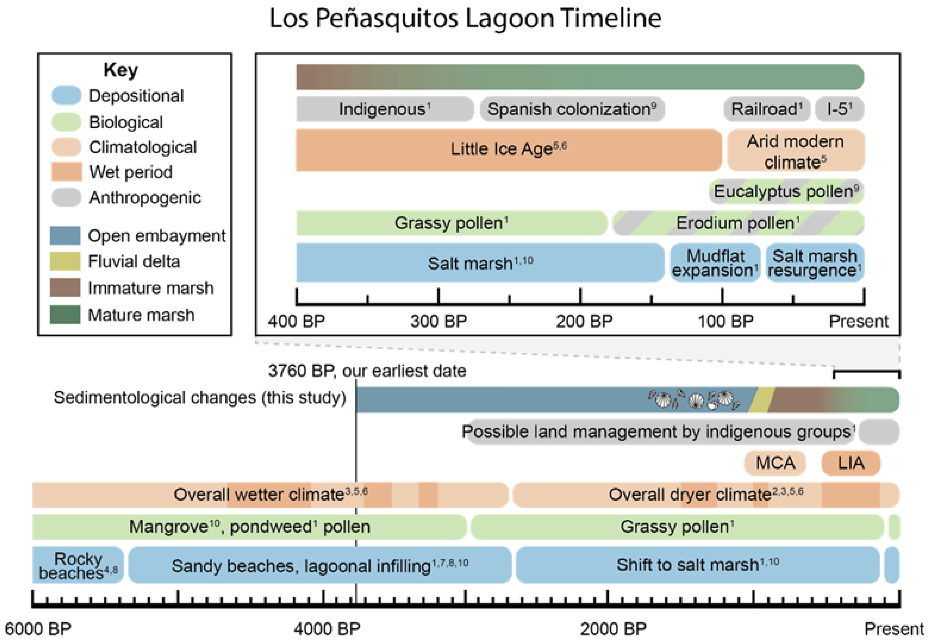
5.3. Paleoenvironmental Reconstruction
5.4. Implications for Restoration and Conservation
6. Conclusions
Author Contributions
Funding
Institutional Review Board Statement
Informed Consent Statement
Data Availability Statement
Conflicts of Interest
References
- Kean, T.H. Protecting America’s Wetlands: An Action Agenda; Food and Agriculture Organization: Rome, Italy, 1988. [Google Scholar]
- Faulkner, S. Urbanization impacts on the structure and function of forested wetlands. Urban Ecosyst. 2004, 7, 89–106. [Google Scholar] [CrossRef]
- Wells, S.; Ravilious, C. In the Front Line: Shoreline Protection and Other Ecosystem Services from Mangroves and Coral Reefs; UNEP/Earthprint: Geneva, Switzerland, 2006. [Google Scholar]
- Leonard, L.A.; Luther, M.E. Flow hydrodynamics in tidal marsh canopies. Limnol. Oceanogr. 1995, 40, 1474–1484. [Google Scholar] [CrossRef]
- Barbier, E.B. Valuing ecosystem services as productive inputs. Econ. Policy 2007, 22, 177–229. [Google Scholar] [CrossRef]
- Temmerman, S.; Meire, P.; Bouma, T.J.; Herman, P.M.J.; Ysebaert, T.A. Ecosystem-based coastal defence in the face of global change. Nature 2013, 504, 79–83. [Google Scholar] [CrossRef] [PubMed]
- Nicholls, R.J. Coastal flooding and wetland loss in the 21st century: Changes under the SRES climate and socio-economic scenarios. Glob. Environ. Change 2004, 14, 69–86. [Google Scholar] [CrossRef]
- Moller, I. Quantifying saltmarsh vegetation and its effect on wave height dissipation: Results from a UK East coast saltmarsh. Estuar. Coast. Shelf Sci. 2006, 69, 337–351. [Google Scholar] [CrossRef]
- Das, S.; Vincent, J.R. Mangroves protected villages and reduced death toll during Indian super cyclone. Proc. Natl. Acad. Sci. USA 2009, 106, 7357–7360. [Google Scholar] [CrossRef] [Green Version]
- Bildstein, K.L.; Bancroft, G.T.; Dugan, P.J.; Gordon, D.H.; Erwin, M.; Nol, E.; Payne, L.X.; Senner, S.E.; The, S.; Bulletin, W.; et al. Approaches to the Conservation of Coastal Wetlands in the Western Hemisphere. Wilson Bull. 1991, 103, 218–254. [Google Scholar]
- Irmler, U.; Heller, K.; Meyer, H.; Reinke, H.-D. Zonation of spiders and carabid beetles (Araneida, Coleoptera: Carabidae) in an inundation gradient of salt marshes at the North and Baltic Sea. Biodivers. Conserv. 2002, 11, 1129–1147. [Google Scholar] [CrossRef]
- Sievers, M.; Brown, C.J.; Tulloch, V.J.D.; Pearson, R.M.; Haig, J.A.; Turschwell, M.P.; Connolly, R.M. The Role of Vegetated Coastal Wetlands for Marine Megafauna Conservation. Trends Ecol. Evol. 2019, 34, 807–817. [Google Scholar] [CrossRef]
- Duarte, C.M.; Middelburg, J.J.; Caraco, N. Major role of marine vegetation on the oceanic carbon cycle. Biogeosciences 2005, 2, 1–8. [Google Scholar] [CrossRef] [Green Version]
- Crooks, S.; Herr, D.; Tamelander, J.; Laffoley, D.; Vandever, J. Mitigating Climate Change through Restoration and Management of Coastal Wetlands and Near-shore Marine Ecosystems: Challenges and Opportunities. Environ. Dep. Pap. 2011, 121, 1–69. [Google Scholar]
- Michener, W.K.; Blood, E.R.; Bildstein, K.L.; Brinson, M.M.; Gardner, L.R. Climate change, hurricanes and tropical storms, and rising sea level in coastal wetlands. Ecol. Appl. 1997, 7, 770–801. [Google Scholar] [CrossRef]
- Morris, J.T.; Sundareshwar, P.; Nietch, C.T.; Kjerfve, B.; Cahoon, D.R. Responses of coastal wetlands to rising sea level. Ecology 2002, 83, 2869–2877. [Google Scholar] [CrossRef]
- Day, J.W.; Christian, R.R.; Boesch, D.M.; Yez-Arancibia, A.; Morris, J.; Twilley, R.R.; Naylor, L.; Schaffner, L.; Stevenson, C. Consequences of climate change on the ecogeomorphology of coastal wetlands. Estuaries Coasts 2008, 31, 477–491. [Google Scholar] [CrossRef]
- Cahoon, D.R.; Guntenspergen, G.R. Climate change, sea-level rise, and coastal wetlands. Natl. Wetl. Newsl. 2010, 32, 8–12. [Google Scholar]
- Day, J.; Ibez, C.; Scarton, F.; Pont, D.; Hensel, P.; Day, J.; Lane, R. Sustainability of Mediterranean Deltaic and Lagoon Wetlands with Sea-Level Rise: The Importance of River Input. Estuaries Coasts 2011, 34, 483–493. [Google Scholar] [CrossRef]
- Kirwan, M.L.; Megonigal, J.P. Tidal wetland stability in the face of human impacts and sea-level rise. Nature 2013, 504, 53–60. [Google Scholar] [CrossRef]
- Van Allen, R.; Schreiner, K.M.; Guntenspergen, G.; Carlin, J. Changes in organic carbon source and storage with sea level rise-induced transgression in a Chesapeake Bay marsh. Estuar. Coast. Shelf Sci. 2021, 261, 107550. [Google Scholar] [CrossRef]
- Syvitski, J.P.; Vörösmarty, C.J.; Kettner, A.J.; Green, P. Impact of humans on the flux of terrestrial sediment to the global coastal ocean. Science 2005, 308, 376–380. [Google Scholar] [CrossRef]
- Braswell, A.E.; Heffernan, J.B.; Kirwan, M.L. How old are marshes on the East Coast, USA? Complex patterns in wetland age within and among regions. Geophys. Res. Lett. 2020, 47, e2020GL089415. [Google Scholar] [CrossRef]
- Spalding, M.; Kainuma, M.; Collins, L. World Atlas of Mangroves; Taylor Francis Group: Abingdon, UK, 2010. [Google Scholar]
- Davidson, N.C. How much wetland has the world lost? Long-term and recent trends in global wetland area. Mar. Freshw. Res. 2014, 65, 934–941. [Google Scholar] [CrossRef]
- Thorne, K.; MacDonald, G.; Guntenspergen, G.; Ambrose, R.; Buffington, K.; Dugger, B.; Freeman, C.; Janousek, C.; Brown, L.; Rosencranz, J. US Pacific coastal wetland resilience and vulnerability to sea-level rise. Sci. Adv. 2018, 4, eaao3270. [Google Scholar] [CrossRef] [PubMed] [Green Version]
- Chapman, V. Wet Coastal Ecosystems; Elsevier Science Ltd.: Amsterdam, The Nederlands, 1978; Volume 1. [Google Scholar]
- Mitsch, W.J.; Gosselink, J.G. Wetlands, 5th ed.; John and Wiley and Sons: Hoboken, NJ, USA, 2015. [Google Scholar]
- Zedler, J.B. The Ecology of Southern California Coastal Salt Marshes: A Community Profile; United States Fish and Wildlife Service: Washington, DC, USA, 1982; p. 110.
- Legg, M.R. Developments in understanding the tectonic evolution of the California Continental Borderland. In From Shoreline to Abyss: Contributions in Marine Geology in Honor of Francis Parker Shepard; Society for Sedimentary Geology: Tulsa, OK, USA, 1991. [Google Scholar]
- Wright, T.L. Structural geology and tectonic evolution of the Los Angeles Basin, California. In Active Margin Basins; American Association of Petroleum Geologists: Tulsa, OK, USA, 1991. [Google Scholar]
- Grant, L.B.; Rockwell, T.K. A northward-propagating earthquake sequence in coastal southern California? Seismol. Res. Lett. 2002, 73, 461–469. [Google Scholar] [CrossRef]
- Grossinger, R.; Stein, E.D.; Cayce, K.; Askevold, R.; Dark, S.; Whipple, A. Historical Wetlands of the Southern California Coast: An Atlas of US Coast Survey T-Sheets, 1851–1889; San Francisco Estuary Institute Oakland: Richmond, CA, USA, 2011. [Google Scholar]
- Emmett, R.; Llansó, R.; Newton, J.; Thom, R.; Hornberger, M.; Morgan, C.; Levings, C.; Copping, A.; Fishman, P. Geographic signatures of North American West Coast estuaries. Estuaries 2000, 23, 765–792. [Google Scholar] [CrossRef]
- Torio, D.D.; Chmura, G.L. Assessing coastal squeeze of tidal wetlands. J. Coast. Res. 2013, 29, 1049–1061. [Google Scholar] [CrossRef]
- Swenson, J.J.; Franklin, J. The effects of future urban development on habitat fragmentation in the Santa Monica Mountains. Landsc. Ecol. 2000, 15, 713–730. [Google Scholar] [CrossRef]
- Steele, E.N. The Rise and Decline of the Olympia Oyster; Fulco Publications: Denville, NJ, USA, 1957. [Google Scholar]
- Polson, M.P.; Zacherl, D.C. Geographic distribution and intertidal population status for the Olympia oyster, Ostrea lurida Carpenter 1864, from Alaska to Baja. J. Shellfish. Res. 2009, 28, 69–77. [Google Scholar] [CrossRef]
- Hopkins, A.E. Attachment of Larvae of the Olympia Oyster, Ostrea Lurida, to Plane Surfaces. Ecology 1935, 16, 82–87. [Google Scholar] [CrossRef]
- Healey, D.; Jackson, J.; Maddox, L.; Shannon, G.; Caulkins, W.; Gray, K.; Nesbitt, P.; Schaub, D.; Stammerjohn, G.; Willard, S.; et al. Torrey Pines State Beach and State Reserve; Department of Parks and Recreation: San Diego, CA, USA, 1984.
- Cole, K.L.; Wahl, E. A late Holocene paleoecological record from Torrey Pines state reserve, California. Quat. Res. 2000, 53, 341–351. [Google Scholar] [CrossRef]
- Scott, D.B.; Mudie, P.J.; Bradshaw, J.S. Coastal evolution of Southern California as interpreted from benthic foraminifera, ostracodes, and pollen. J. Foraminifer. Res. 2011, 41, 285–307. [Google Scholar] [CrossRef]
- Mudie, P.J.; Byrne, R. Pollen Evidence for Historic Sedimentation Rates in California Coastal Marshes. Estuar. Coast. Mar. Sci. 1980, 10, 305–316. [Google Scholar] [CrossRef]
- Stein, E.D.; Cayce, K.; Salomon, M.; Bram, D.L.; De Mello, D.; Grossinger, R.; Dark, S. Wetlands of the Southern California coast: Historical extent and change over time. South. Calif. Coast. Water Res. Proj. Tech. Rep. 2014, 826, 1–50. [Google Scholar]
- Baker, P. Review of ecology and fishery of the Olympia oyster, Ostrea lurida with annotated bibliography. J. Shellfish. Res. 1995, 14, 501–518. [Google Scholar]
- Inman, D.L. Application of coastal dynamics to the reconstruction of paleocoastlines in the vicinity of La Jolla, California. In Quaternary Coastlines and Marine Archaeology; Masters, P.M., Flemming, M.C., Eds.; Academic Press: London, UK, 1983; pp. 1–49. [Google Scholar]
- Reynolds, L.C.; Simms, A.R. Late Quaternary relative sea level in Southern California and Monterey Bay. Quat. Sci. Rev. 2015, 126, 57–66. [Google Scholar] [CrossRef]
- Masters, P.M. Holocene sand beaches of southern California: ENSO forcing and coastal processes on millennial scales. Palaeogeogr. Palaeoclimatol. Palaeoecol. 2006, 232, 73–95. [Google Scholar] [CrossRef]
- Masters, P.M.; Gallegos, D.R. Environmental change and coastal adaptations in San Diego County during the Middle Holocene. In Archaeology of the California Coast during the Middle Holocene; Institute of Archaeology, University of California: Los Angeles, CA, USA, 1997. [Google Scholar]
- Scott, D.B.; Mudie, P.J.; Bradshaw, J.S. Benthonic foraminifera of three southern Californian lagoons; ecology and Recent stratigraphy. J. Foraminifer. Res. 1976, 6, 59–75. [Google Scholar] [CrossRef]
- Cole, K.L.; Liu, G.-W. Holocene paleoecology of an estuary on Santa Rosa Island, California. Quat. Res. 1994, 41, 326–335. [Google Scholar] [CrossRef]
- Davis, O.K. Rapid climatic change in coastal southern California inferred from pollen analysis of San Joaquin Marsh. Quat. Res. 1992, 37, 89–100. [Google Scholar] [CrossRef]
- Mensing, S.; Byrne, R. Pre-mission invasion of Erodium cicutarium in California. J. Biogeogr. 1998, 25, 757–762. [Google Scholar] [CrossRef]
- Bulseco, A. A synopsis of the Olympia oyster (Ostrea lurida). Aquaculture 1982, 262, 63–72. [Google Scholar]
- MacKenzie, C.L. History of oystering in the United States and Canada featuring the eight greatest oyster estuaries. Mar. Fish. Rev. 1996, 58, 1–78. [Google Scholar]
- Pritchard, C.; Shanks, A.; Rimler, R.; Oates, M.; Rumrill, S. The Olympia oyster Ostrea lurida: Recent advances in natural history, ecology, and restoration. J. Shellfish. Res. 2015, 34, 259–271. [Google Scholar] [CrossRef]
- Seale, E.M.; Zacherl, D.C. Seasonal settlement of Olympia oyster larvae, Ostrea lurida Carpenter 1864 and its relationship to seawater temperature in two southern California estuaries. J. Shellfish. Res. 2009, 28, 113–120. [Google Scholar] [CrossRef]
- Trimble, A.C.; Ruesink, J.L.; Dumbauld, B.R. Factors Preventing the Recovery of a Historically Overexploited Shellfish Species, Ostrea lurida Carpenter 1864. J. Shellfish. Res. 2009, 28, 97–106. [Google Scholar] [CrossRef]
- Leidelmeijer, J.A.; Kirby, M.E.C.; MacDonald, G.; Carlin, J.A.; Avila, J.; Han, J.; Nauman, B.; Loyd, S.; Nichols, K.; Ramezan, R. Younger Dryas to early Holocene (12.9 to 8.1 ka) limnological and hydrological change at Barley Lake, California (northern California Coast Range). Quat. Res. 2021, 103, 193–207. [Google Scholar] [CrossRef]
- Blott, S.J.; Pye, K. Gradistat: A grain size distribution and statistics package for the analysis of unconsolidated sediments. Earth Surf. Processes Landf. 2001, 26, 1237–1248. [Google Scholar] [CrossRef]
- Dean, W.E., Jr. Determination of Carbonate and Organic Matter in Calcareous Sediments and Sedimentary Rocks by Loss on Ignition: Comparison with Other Methods. SEPM J. Sediment. Res. 1974, 44, 242–248. [Google Scholar] [CrossRef] [Green Version]
- Santisteban, J.I.; Mediavilla, R.; Lopez-Pamo, E.; Dabrio, C.J.; Zapata, M.B.R.; Garcia, M.J.G.; Castano, S.; Martinez-Alfaro, P.E. Loss on ignition: A qualitative or quantitative method for organic matter and carbonate mineral content in sediments? J. Paleolimnol. 2004, 32, 287–299. [Google Scholar] [CrossRef] [Green Version]
- Heiri, O.; Lotter, A.F.; Lemcke, G. Loss on ignition as a method for estimating organic and carbonate content in sediments: Reproducibility and comparability of results. J. Paleolimnol. 2001, 25, 101–110. [Google Scholar] [CrossRef]
- Behrensmeyer, A.K.; Kidwell, S.M.; Gastaldo, R.A. Taphonomy and paleobiology. Paleobiology 2000, 26, 103–147. [Google Scholar] [CrossRef]
- Kidwell, S.M. Taphonomic expressions of sedimentary hiatuses: Field observations on bioclastic concentrations and sequence anatomy in low, moderate and high subsidence settings. Geol. Rundsch. 1993, 82, 189–202. [Google Scholar] [CrossRef]
- Kidwell, S.M.; Fursich, F.T.; Aigner, T. Conceptual Framework for the Analysis and Classification of Fossil Concentrations. Palaios 1986, 1, 228. [Google Scholar] [CrossRef]
- Brandt, D.S. Taphonomic grades as a classification for fossiliferous assemblages and implications for paleoecology. Palaios 1989, 4, 303–309. [Google Scholar] [CrossRef]
- Flessa, K.W.; Cutler, A.H.; Meldahl, K.H.; Paleobiology, S.; Spring, N.; Flessa, K.W.; Cutler, A.H.; Meldahl, K.H. Time and Taphonomy: Quantitative Estimates of Time-Averaging and Stratigraphic Disorder in a Shallow Marine Habitat. Paleobiology 1993, 19, 266–286. [Google Scholar] [CrossRef]
- Stuiver, M.; Reimer, P.J.; Reimer, R.W. Calib 8.2. Available online: http://calib.org (accessed on 5 November 2020).
- Ingram, B.L.; Southon, J.R. Reservoir ages in Eastern Pacific coastal and estuarine waters. Radiocarbon 1996, 38, 573–582. [Google Scholar] [CrossRef] [Green Version]
- Stevenson, R.E.; Emery, K.O. Marshlands at Newport Bay, California; Allan Hancock Foundation: Santa Maria, CA, USA, 1958. [Google Scholar]
- Leeper, R.; Rhodes, B.; Kirby, M.; Scharer, K.; Carlin, J.; Hemphill-Haley, E.; Avnaim-Katav, S.; MacDonald, G.; Starratt, S.; Aranda, A. Evidence for coseismic subsidence events in a southern California coastal saltmarsh. Sci. Rep. 2017, 7, 44615. [Google Scholar] [CrossRef] [Green Version]
- Reynolds, L.C.; Simms, A.R.; Ejarque, A.; King, B.; Anderson, R.S.; Carlin, J.A.; Bentz, J.M.; Rockwell, T.K.; Peters, R. Coastal flooding and the 1861–1862 California storm season. Mar. Geol. 2018, 400, 49–59. [Google Scholar] [CrossRef] [Green Version]
- Zurbuchen, J.; Simms, A.R.; Huot, S. Episodic Coastal Progradation of the Oxnard Plain, Southern California, USA. J. Coast. Res. 2020, 36, 1130–1144. [Google Scholar] [CrossRef]
- Simms, A.; Reynolds, L.C.; Bentz, M.; Roman, A.; Rockwell, T.; Peters, R. Tectonic subsidence of California estuaries increases forecasts of relative sea-level rise. Estuaries Coasts 2016, 39, 1571–1581. [Google Scholar] [CrossRef]
- Ramcharan, E.K.; McAndrews, J.H. Holocene development of coastal wetland at Maracas Bay, Trinidad, West Indies. J. Coast. Res. 2006, 22, 581–586. [Google Scholar] [CrossRef]
- Covault, J.A.; Romans, B.W.; Fildani, A.; McGann, M.; Graham, S.A. Rapid Climatic Signal Propagation from Source to Sink in a Southern California Sediment-Routing System. J. Geol. 2010, 118, 247–259. [Google Scholar] [CrossRef] [Green Version]
- Kirby, M.; Lund, S.; Patterson, W.; Anderson, M.; Bird, B.; Ivanovici, L.; Monarrez, P.; Nielsen, S. A Holocene record of Pacific decadal oscillation (PDO)-related hydrologic variability in southern California (Lake Elsinore, CA). J. Paleolimnol. 2010, 44, 819–839. [Google Scholar] [CrossRef] [Green Version]
- Kirby, M.E.C.; Patterson, W.P.; Lachniet, M.; Noblet, J.A.; Anderson, M.A.; Nichols, K.; Avila, J. Pacific Southwest United States holocene droughts and pluvials inferred from sediment δ18O (calcite) and grain size data (Lake Elsinore, California). Front. Earth Sci. 2019, 7, 1–14. [Google Scholar] [CrossRef]
- Kirby, M.E.; Lund, S.P.; Anderson, M.A.; Bird, B.W. Insolation forcing of Holocene climate change in Southern California: A sediment study from Lake Elsinore. J. Paleolimnol. 2007, 38, 395–417. [Google Scholar] [CrossRef]
- Cayan, D.R.; Redmond, K.T.; Riddle, L.G. ENSO and hydrologic extremes in the western United States. J. Clim. 1999, 12, 2881–2893. [Google Scholar] [CrossRef] [Green Version]
- Gray, A.B.; Pasternack, G.B.; Watson, E.B.; Warrick, J.A.; Goñi, M.A. The effect of El Niño Southern Oscillation cycles on the decadal scale suspended sediment behavior of a coastal dry-summer subtropical catchment. Earth Surf. Processes Landf. 2015, 40, 272–284. [Google Scholar] [CrossRef] [Green Version]
- Inman, D.L.; Jenkins, S.A. Climate change and the episodicity of sediment flux of small California rivers. J. Geol. 1999, 107, 251–270. [Google Scholar] [CrossRef] [Green Version]
- Gray, A.B.; Pasternack, G.B.; Watson, E.B. Estuarine abandoned channel sedimentation rates record peak fluvial discharge magnitudes. Estuar. Coast. Shelf Sci. 2018, 203, 90–99. [Google Scholar] [CrossRef]
- Gray, A.B.; Warrick, J.A.; Pasternack, G.B.; Watson, E.B.; Goi, M.A. Suspended sediment behavior in a coastal dry-summer subtropical catchment: Effects of hydrologic preconditions. Geomorphology 2014, 214, 485–501. [Google Scholar] [CrossRef] [Green Version]
- Fraticelli, C.M. Climate Forcing in a Wave-Dominated Delta: The Effects of Drought—Flood Cycles on Delta Progradation. J. Sediment. Res. 2006, 76, 1067–1076. [Google Scholar] [CrossRef]
- Carlin, J.A.; Schreiner, K.M.; Dellapenna, T.M.; McGuffin, A.; Smith, R.W. Evidence of recent flood deposits within a distal shelf depocenter and implications for terrestrial carbon preservation in non-deltaic shelf settings. Mar. Geol. 2021, 431, 106376. [Google Scholar] [CrossRef]
- Uk, D.F.; Uk, G.F.; Zealand, N.; France, M.K. Information from paleoclimate archives. Clim. Change 2013 Phys. Sci. Basis Work. Group I Contrib. Fifth Assess. Rep. Intergov. Panel Clim. Change 2013, 9781107057, 383–464. [Google Scholar] [CrossRef]
- Masson-Delmotte, V.; Schulz, M.; Abe-Ouchi, A.; Beer, J.; Ganopolski, A.; González Rouco, J.; Jansen, E.; Lambeck, K.; Luterbacher, J.; Naish, T. Information from paleoclimate archives. In Climate Change 2013: The Physical Science Basis. Contribution of Working Group I to the Fifth Assessment Report of the Intergovernmental Panel on Climate Change; Stocker, T., Qin, D., Plattner, G.-K., Tignor, M., Allen, S., Boschung, J., Nauels, A., Xia, Y., Bex, V., Midgley, P., Eds.; Cambridge University Press: Cambridge, UK, 2013; Volume 383464, pp. 383–464. [Google Scholar]
- MacDonald, G.M. Severe and sustained drought in southern California and the West: Present conditions and insights from the past on causes and impacts. Quat. Int. 2007, 173, 87–100. [Google Scholar] [CrossRef]
- Mann, M.E.; Zhang, Z.; Rutherford, S.; Bradley, R.S.; Hughes, M.K.; Shindell, D.; Ammann, C.; Faluvegi, G.; Ni, F. Medieval Climate Anomaly. Science 2009, 78, 1256–1260. [Google Scholar] [CrossRef] [PubMed] [Green Version]
- Heusser, L.E.; Hendy, I.L.; Barron, J.A. Vegetation response to southern California drought during the Medieval Climate Anomaly and early Little Ice Age (AD 800-1600). Quat. Int. 2015, 387, 23–35. [Google Scholar] [CrossRef] [Green Version]
- Correggiari, A.; Cattaneo, A.; Trincardi, F. The modern Po Delta system: Lobe switching and asymmetric prodelta growth. Mar. Geol. 2005, 222, 49–74. [Google Scholar] [CrossRef]
- Carlin, J.A.; Dellapenna, T.M. The evolution of a subaqueous delta in the Anthropocene: A stratigraphic investigation of the Brazos River delta, TX USA. Cont. Shelf Res. 2015, 111, 139–149. [Google Scholar] [CrossRef]
- Lamb, H.H. The early medieval warm epoch and its sequel. Palaeogeogr. Palaeoclimatol. Palaeoecol. 1965, 1, 13–37. [Google Scholar] [CrossRef]
- MacDonald, G.M.; Case, R.A. Variations in the Pacific Decadal Oscillation over the past millennium. Geophys. Res. Lett. 2005, 32, L08703. [Google Scholar] [CrossRef] [Green Version]
- MacDonald, G.M.; Kremenetski, K.V.; Hidalgo, H.G. Southern California and the perfect drought: Simultaneous prolonged drought in southern California and the Sacramento and Colorado River systems. Quat. Int. 2008, 188, 11–23. [Google Scholar] [CrossRef]
- Kirby, M.X.; Linares, O.F. Fishing down the coast: Historical expansion and collapse of oyster fisheries along continental margins. Proc. Natl. Acad. Sci. USA 2004, 101, 13096–13099. [Google Scholar] [CrossRef] [PubMed] [Green Version]


| Grain Size Distribution as Percentages of Total | ||||||
|---|---|---|---|---|---|---|
| Minimum | Maximum | Mean | Standard Deviation | n | Sorting | |
| Unit 1 | ||||||
| Mud | 8.6 | 39.6 | 23.4 | 8.5 | 91 | 2.5 µm |
| Fine Sand | 40.6 | 76.3 | 65 | 6.8 | 91 | |
| Coarse Sand | 3.4 | 32.9 | 11.6 | 6.4 | 91 | |
| Unit 2 | ||||||
| Mud | 5.7 | 66.3 | 24.8 | 15.6 | 59 | |
| Fine Sand | 14 | 56.9 | 32.7 | 9.7 | 59 | 3.7 µm |
| Coarse Sand | 14.4 | 67.4 | 42.5 | 14.1 | 59 | |
| Unit 3 | ||||||
| Mud | 48.4 | 73.1 | 63 | 7.3 | 15 | |
| Fine Sand | 24.1 | 49.4 | 34.6 | 7.4 | 15 | 3.1 µm |
| Coarse Sand | 0 | 7.1 | 2.4 | 1.6 | 15 | |
| Unit 4 | ||||||
| Mud | 73.7 | 99.9 | 91.8 | 6 | 29 | |
| Fine Sand | 0.1 | 18.8 | 7.2 | 5.2 | 29 | 2.8 µm |
| Coarse Sand | 0 | 7.5 | 1 | 1.6 | 29 | |
| Unit | 1 | 2 | 3 | 4 |
|---|---|---|---|---|
| 1 | - | <0.001 | <0.001 | <0.001 |
| 2 | - | - | <0.001 | <0.001 |
| 3 | - | - | - | <0.001 |
| 4 | - | - | - | - |
| Species | Class | Environment | Whole Samples | Shell Fragments |
|---|---|---|---|---|
| Ostrea lurida | Bivalvia | Hypersaline, marine, brackish | 2 | 6 |
| Argopecten ventricosus | Bivalvia | Marine | 3 | 0 |
| Chione undatella | Bivalvia | Marine | 2 | 4 |
| Macoma nasuta | Bivalvia | Marine | 6 | 3 |
| Tagelus californiensis | Bivalvia | Marine | 1 | 11 |
| Cerithideopsis californica | Gastropoda | Brackish | 8 | 25 |
| Nassarius tegula | Gastropoda | Marine | 1 | 0 |
| Total Shells | 23 | 49 |
| Sample ID | Sample Depth (cm) | Material Dated | Uncalibrated 14C Age (BP) | ±Error | Calibrated 14 C Age Range (BP) | Median Calibrated Age (BP) |
|---|---|---|---|---|---|---|
| LPL07 158 | 158 | Plant material | 1165 | 35 | 1044–1155 | 1100 |
| LPL07 SH1 | 165–185 | Argopecten ventricosus | 1975 | 25 | 1273–1572 | 1422 |
| LPL07 SH2 | 165–185 | Macoma nasuta | 1660 | 20 | 945–1254 | 1100 |
| LPL07 SH3 | 165–185 | Tagelus californiensis | 1975 | 25 | 1272–1572 | 1422 |
| LPL07 SH4 | 165–185 | Cerithideopsis californica | 1990 | 20 | 1284–1583 | 1434 |
| LPL07 SH5 | 165–185 | Chione undatella | 1595 | 20 | 878–1200 | 1039 |
| LPL07 OL1 | 190 | Ostrea lurida | 2130 | 20 | 1406–1746 | 1576 |
| LPL07 OL2 | 190 | Ostrea lurida | 2230 | 20 | 1533–1874 | 1704 |
| LPL07 240 | 240 | Plant material | 3375 | 20 | 3563–3646 | 3605 |
| LPL04 OL | 91 | Ostrea lurida | 1415 | 20 | 682–981 | 832 |
| LPL04 236 | 158 | Plant material | 3510 | 15 | 3715–3805 | 3760 |
| LPL03 170 | 165–185 | Plant material | 2460 | 25 | 2405–2546 | 2476 |
| Unit | Key Sedimentary Characteristics | Interpretation |
|---|---|---|
| 1 | Dominated by fine sand (~70%) | Open embayment |
| Generally consistent grain size throughout | ||
| TOM < 10% | ||
| Shell hash layer | ||
| 2 | Dominated by fine (~30%) and coarse (~40%) sand | Fluvial delta |
| Fluctuating grain size | ||
| TOM < 15% | ||
| 3 | Dominated by fine sand (~35%) and mud (~60%) | Immature marsh |
| Trace amounts of coarse sand | ||
| Fining upward trend | ||
| TOM ≤ 15% | ||
| 4 | Dominated by mud (~90%) | Mature marsh |
| Small amounts of both fine and coarse sand | ||
| TOM > 15% |
Publisher’s Note: MDPI stays neutral with regard to jurisdictional claims in published maps and institutional affiliations. |
© 2022 by the authors. Licensee MDPI, Basel, Switzerland. This article is an open access article distributed under the terms and conditions of the Creative Commons Attribution (CC BY) license (https://creativecommons.org/licenses/by/4.0/).
Share and Cite
Dickson, S.; Carlin, J.; Bonuso, N.; Kirby, M.E. Documenting the Evolution of a Southern California Coastal Lagoon during the Late Holocene. Coasts 2022, 2, 102-124. https://doi.org/10.3390/coasts2020007
Dickson S, Carlin J, Bonuso N, Kirby ME. Documenting the Evolution of a Southern California Coastal Lagoon during the Late Holocene. Coasts. 2022; 2(2):102-124. https://doi.org/10.3390/coasts2020007
Chicago/Turabian StyleDickson, Sarah, Joseph Carlin, Nicole Bonuso, and Matthew E. Kirby. 2022. "Documenting the Evolution of a Southern California Coastal Lagoon during the Late Holocene" Coasts 2, no. 2: 102-124. https://doi.org/10.3390/coasts2020007