Article

Qualitative Model of the Causal Interactions between Phytoplankton, Zooplankton, and Environmental Factors in the Romanian Black Sea

1
Ecology and Marine Biology Department, National Institute for Marine Research and Development “Grigore Antipa”, 300 Mamaia Blvd., 900581 Constanta, Romania
2
National Institute for Marine Research and Development “Grigore Antipa”, 300 Mamaia Blvd., 900581 Constanta, Romania
3
Chemical Oceanography and Marine Pollution Department, National Institute for Marine Research and Development “Grigore Antipa”, 300 Mamaia Blvd., 900581 Constanta, Romania
*
Authors to whom correspondence should be addressed.
Phycology 2024, 4(1), 168-189; https://doi.org/10.3390/phycology4010010
Submission received: 26 January 2024 / Revised: 18 March 2024 / Accepted: 20 March 2024 / Published: 21 March 2024

Abstract

:
In order to analyze how environmental factors affect planktonic organisms along the Romanian Black Sea coast, this study created semi-quantitative models of the causal relationships between phytoplankton, zooplankton, and physicochemical parameters by utilizing user-friendly modeling tools. Eleven years of time-series data (March–September 2008–2018) were used to investigate the relationships between phytoplankton, zooplankton, and environmental factors (such as temperature, salinity, and nutrients). Variables such as marine reporting units and phytoplankton species and classes were used to identify developmental patterns, utilizing the Mental Modeler platform to consider interactions between the physicochemical parameters and phytoplankton, phytoplankton and zooplankton, and zooplankton and physicochemical parameters. Although the increase in the overall number of elements and linkages was uncertain in waters with variable salinity compared to marine ones, the semi-quantitative models created for the three marine reporting units along the Romanian Black Sea coast were comparable in terms of complexity. Across the typical and examined types of phytoplankton proliferation (normal, abundant, and blooms), the number of components and connections in the case of phytoplankton blooms substantially decreased as species- and growth-promoting variables increased.

1. Introduction

Despite the highly different levels of phylogenetic, biochemical, metabolic, and ecological variability, marine plankton is widely distributed throughout the marine ecosystem and plays a significant role in controlling the biological pump and global biochemical cycles [1,2,3]. Because plankton adapt quickly to environmental changes, they are valuable biological indicators of the trophic condition of an aquatic ecosystem and its water quality [3].
Since phytoplankton is a primary producer and can influence higher trophic levels by providing zooplankton and other invertebrates with nutritional bases, a direct correlation exists between the density of phytoplankton and the productivity of an aquatic environment [4,5]. Their productions are directly correlated with physicochemical parameters, and seasonal temperature variations may be a controlling element in their growth and diversity, in addition to other variables [4].
In today’s aquatic environment, plankton communities face a unique set of difficulties, including the effects of climate change on ecosystems. Comprehending the interplay between the dynamics of plankton communities and the current human-driven climate change is, therefore, crucial and a major global challenge. Changes in the environment can have a direct or indirect impact on the physiological characteristics and behavioral aspects of marine plankton. This can result in changes to these organisms’ abundance, spatial range, and community structure [6,7]. Since marine plankton is the basis of the ocean’s life-support systems, these changes, therefore, result in changes in biological interactions (e.g., trophic cascades, species competition, and facilitation) and ecosystem functioning (e.g., elemental cycling) [8]. Thus, it is crucial to comprehend how marine plankton reacts to external driving factors [3].
Not only do phytoplankton and zooplankton frequently inhabit aquatic areas, but they also make up the entire aquatic ecosystem. Researchers have placed strong emphasis on the global increase in dangerous phytoplankton blooms over the past 20 years, but little is known about how harvesting affects phytoplankton–zooplankton communities [9].
The quantity of plankton in a water body determines the productivity of that ecosystem [10]. The essential biological elements that provide energy to higher organisms via the food chain are phytoplankton and zooplankton [11], which are trustworthy resources for assessing the levels of water contamination and function as bioindicators [12]. Plankton is, therefore, essential to the health of ecosystems and provides a variety of ecosystem services (ES), such as acting as a sink for CO2 in order to regulate the climate and forming the foundation of food webs that support the production of higher trophic levels [13].
Fuzzy cognitive mapping is a technique for assessing and quantitatively contrasting the opinions of various actors regarding ecosystem structures. The models’ responses to different pressure conditions can be demonstrated through simulations and quantitative comparisons. This can show discrepancies in the beliefs about critical interactions in an ecosystem and about how a system will react to management activities that help experts to understand the impact associated with environmental changes and develop strategies for reducing unwanted outcomes by capturing, communicating, and representing knowledge [14].
Fuzzy-ogic Cognitive Mapping (FCM) was created in 1986 to organize expert knowledge through a “fuzzy” systems programming technique modeled after the decision-making process of the human mind. Due to their adaptability, FCMs were developed to investigate how an environmental issue is perceived or simulate a complicated system with a lot of uncertainty and when few empirical data are available [15]. To depict the linkages and interactions between the variables in FCMs, arrows are used to connect the variables, which are also known as concepts [16,17]. The numbers indicating the interaction’s strength and whether it is positive or negative also indicate the type and strength of the interaction. According to Jeter and Kok [18] and Özesmi and Özesmi [19], a positive interaction denotes an increase in one idea, while a negative interaction denotes a decline in another concept.
By building cognitive knowledge maps (FCMs), the Mental Modeler enables the development of the semi-quantitative model that (1) defines the essential components, (2) defines the strength of the relationships between the components, and (3) runs scenarios that determine how the system reacts in certain conditions [20].
This study aims to determine the causal linkages between phytoplankton, zooplankton, and environmental parameters using an eleven-year data set collected between 2008 and 2018 (March–September). With the use of semi-quantitative models, the dynamics of the pelagic habitat are captured, and the “nodes” of the network are identified, representing the attributes of the ecosystem that can be modified in different scenarios. The main purpose of this tool is to understand the changes that occur in the ecosystem. With the aid of cognitive maps, phytoplankton developmental patterns were identified, considering the influence exerted by physico-chemical factors and the zooplankton community.

2. Materials and Methods

The Black Sea, with an average salinity ranging from 17 to 18 g/L, displays a pronounced stratified structure, featuring distinct biogeochemical layers. Its hydrographic pattern consists of surface waters with low salinity, originating from rivers, overlaying deep Mediterranean-origin waters with higher salinity. Between these layers, there exists a well-defined and enduring pycnocline, limiting the vertical mixing depth to 100–150 m. The oxic layer extends to approximately 50 m and aligns with the euphotic zone and the boundary of the pelagic habitat. This layer facilitates robust biological processes, boasting high oxygen concentrations around 300 µM, which are subject to seasonal fluctuations in nutrients and organic matter received from rivers and coastal areas. The Black Sea’s mean thermohaline state is governed by the balance of water and salinity (dilution at the surface and salinification by the Mediterranean inflow), while air–sea heat exchange shapes seasonal variability. In coastal zones, the oxycline, denoting a distinct oxygen gradient, begins at depths of 70–100 m. Below this lies the suboxic layer, situated at depths of 100–130 m, which is characterized by diminished oxygen levels (<10 µM) and escalating hydrogen sulfide concentrations. Descending further, the anoxic layer begins at depths of 150–200 m and is devoid of oxygen, except for sustaining sulfate-reducing bacteria through hydrogen sulfide [21,22,23,24].
The climate in the Black Sea region is temperate-continental. Summers experience relatively uniform air temperatures, while winters exhibit temperature variations according to geographical locations, with minimums in the northwest and maximums in the southeast. Water temperatures fluctuate seasonally, reaching up to 25 °C in summer (occasionally up to 28 °C) and dropping to 6–8 °C in winter. The northwest coast experiences winter ice, while the southeast remains around 9 °C [25].
Typically, the offshore waters of the Black Sea lack vertical circulation, which is primarily attributed to significant density stratification. This stratification inhibits deep convection processes. The currents in the Black Sea are predominantly horizontal, precluding the occurrence of the permanent upwelling and downwelling phenomena observed in other regions of the planetary ocean [26].
The hydrological and hydro-chemical attributes of the coastal water bodies in the Black Sea exhibit notable variations. The coastal marine environment undergoes rapid and substantial changes in both spatial and temporal dimensions compared to shelf waters. The plankton community near the shore is not only influenced by river flow but also by local coastal runoff, encompassing sewage and agricultural drains, various human activities, local wind-driven surface currents leading to upwelling and downwelling, and additional natural and anthropogenic factors [27,28].
The samples were collected between 2008 and 2018 (March to September, in spring and summer seasons) along the Romanian Black Sea coast (Table S1) within three marine reporting units (MRU). The sampling network covered 40 stations, of which, 9 stations were in waters with variable salinity, 14 stations were in coastal waters, and 17 stations were in marine shelf waters (Figure 1 and Table S1). Seawater and biological (phytoplankton and zooplankton) samples were collected from standard depths (0, 10, 20, 30, 50, 70, and bottom) from stations with maximum depths of 100 m.
For the investigation of phytoplankton communities (taxonomic structure, numerical abundance, and biomass), 500 mL seawater samples were collected using 5 L Teflon Niskin. The samples were fixed immediately with formaldehyde at a 37% concentration. In the laboratory, the samples were concentrated using the sedimentation method down to approx. 30 mL by settling and removing the supernatant in two stages. This was performed once every two weeks [29] (Moncheva and Parr, 2010). Each sample was then homogenized, and a sample fraction of 0.1/1 mL was completely analyzed under an inverted microscope (Olympus IX73). For the identification of the species, we used both identification keys [30,31,32,33] and online databases (World Register of Marine Species, Nordic Microalgae, AlgaeBase). All microalgae encountered were identified at the level of species, genus, or algal group, counting all the cells of each species/genus/group encountered. With the primary data thus obtained, the abundance (cells/L) and wet biomass (mg/m3) were calculated for each species and for the highest taxonomic level that could be identified. The individual cell biovolume (V, μm3) was derived via measurements through the approximation of the cell shape of each species to the most similar regular solid. This was calculated by utilizing the respective formulas used routinely in the lab, working according to the MISIS project inter-calibration exercise [34]. Cell biovolume was converted into weight (W, ng) following the method of Hutchinson [35]. The taxonomic nomenclature was updated according to the World Register of Marine Species (WoRMS).
Zooplankton samples were collected by employing vertical tows, with a Juday net (0.1 m2 mouth opening area, 150 μm mesh size) equipped with a flow meter used to estimate the filtered water volume [36]. The zooplankton samples were subjected to both quantitative and qualitative assessments using an Olympus SZX10 stereomicroscope. To identify the taxonomic affiliation of zooplankton and determine species, we referred to appropriate manuals and guides [37,38]. The classification of identified taxa was carried out, following the World Register of Marine Species (WoRMS). Not all organisms could be identified at the species level; meroplanktonic elements were only identified at the group level. In the subsample(s) examined in the Bogorov chamber, all organisms were counted until a minimum of 100 individuals were recorded for each of the three dominant taxonomic groups. For large organisms, the entire sample was examined in a Petri dish. We employed the count of individuals and mean individual weights to estimate the density in ind/m3 and biomass in mg/m3 of wet weight, respectively. These estimations were based on the tables of constant weight for Black Sea zooplankton [36,39].
Temperature and salinity were measured using the reversible thermometer, the titration method, and the CastAway CTD multiparameter probe (YSI Cast Away model). Dissolved nutrient concentrations were determined according to the standard methods used for seawater analysis [40]. Thus, nutrients were quantified via spectrophotometric analytical methods validated in the laboratory and having as reference the manual “Methods of Seawater Analysis” [40] and investigations into nitrate we used as references (Mullin and Riley, 1955) [41]. The methods were manual, and each sample was treated individually and manually for each parameter. The determination of nitrate was based on the method of Mullin and Riley (1955) [41]. Nitrate was reduced to nitrite using hydrazine sulfate. The nitrite produced was reacted with sulfanilamide in an acid solution. The resulting diazonium compound was coupled with N-(1-Naphthyl)-ethylenediamine dihydrochloride to form a colored azo dye, the extinction of which can be measured spectrophotometrically.
The determination of ammonia was based on the indophenol blue method [40], where ammonia reacts with hypochlorite in a moderately alkaline solution to give monochloramine which, in the presence of phenol, catalytic amounts of nitroprusside ions, and excess hypochlorite, gives indophenol blue.
The inorganic phosphate ions present in water reacted with ammonium molybdate in an acidic medium to form a yellowish phosphomolybdenum complex. This complex was immediately reduced to a blue-colored compound, whose intensity was proportional to the concentration of phosphate ions. The intensity of the blue color was measured with a spectrophotometer in the visible range and had a wavelength of 885 nm [40].
The silicon ions reacted with ammonium molybdate in an acidic medium to form a yellowish silicomolybdenum complex. In the presence of a reducing agent (ascorbic acid), the complex was reduced to an intensely blue-colored compound, the intensity of the color being proportional to the concentration of silicon present in the water. The intensity of the blue color was measured with a spectrophotometer in the visible range and had a wavelength of 810 nm [40].
Data analyses were conducted using PRIMER v. 7.0 [42], and statistical analysis was performed via XLSTAT [43] and Statistica® 14.0.1.25 (TIBCO Software Inc., Palo Alto, CA, USA) [44]. The semi-quantitative modeling was carried out with the Mental Modeler software (open-source, https://www.mentalmodeler.com/) (accessed on 15 January 2024) by using significant correlation coefficients to indicate the strength of the linkages between components [20]. FCM produced qualitative static models that were subsequently transformed into quantitative dynamic models. It encapsulated knowledge by specifying the three key attributes of a system: the constituents of the system (plankton and abiotic parameters), the positive or negative associations between these constituents, and the extent of influence one component can exert on another. This influence was characterized using qualitative weightings such as high, medium, or low, with significant Pearson correlation coefficients serving as the basis for these qualitative weightings [14,20]. For model development, the Mental Modeler software (http://www.mentalmodeler.org/) (accessed on 15 January 2024) was utilized to input the noteworthy (p < 0.05) Pearson correlation coefficients. These were obtained between physicochemical parameters and planktonic components and were based on marine reporting units. In the visualization, positive correlations are depicted as blue arrows, while negative correlations are represented as orange arrows. The weightings of these correlations are reflective of the coefficient values.
Spatial distribution maps were produced with ArcGIS Desktop 10.7 [45]. GIS modeling tools are employed for spatial interpolation, a technique that predicts the values of unsampled points or data gaps within a study area [46]. Using this method proves particularly valuable in examining extensive marine environments, where constraints such as time and financial resources hinder comprehensive data collection across entire study areas [47]. Spatial interpolation involves predicting the value of a variable at a location where it has not been directly measured based on data collected at known locations. In our study, we utilized local interpolators, specifically inverse distance weighting (IDW) [46,47].

3. Results

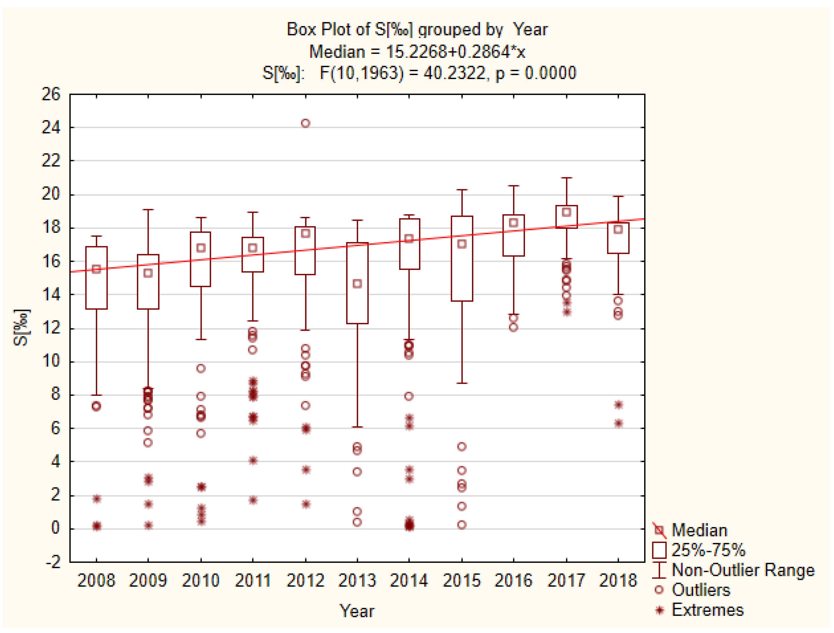
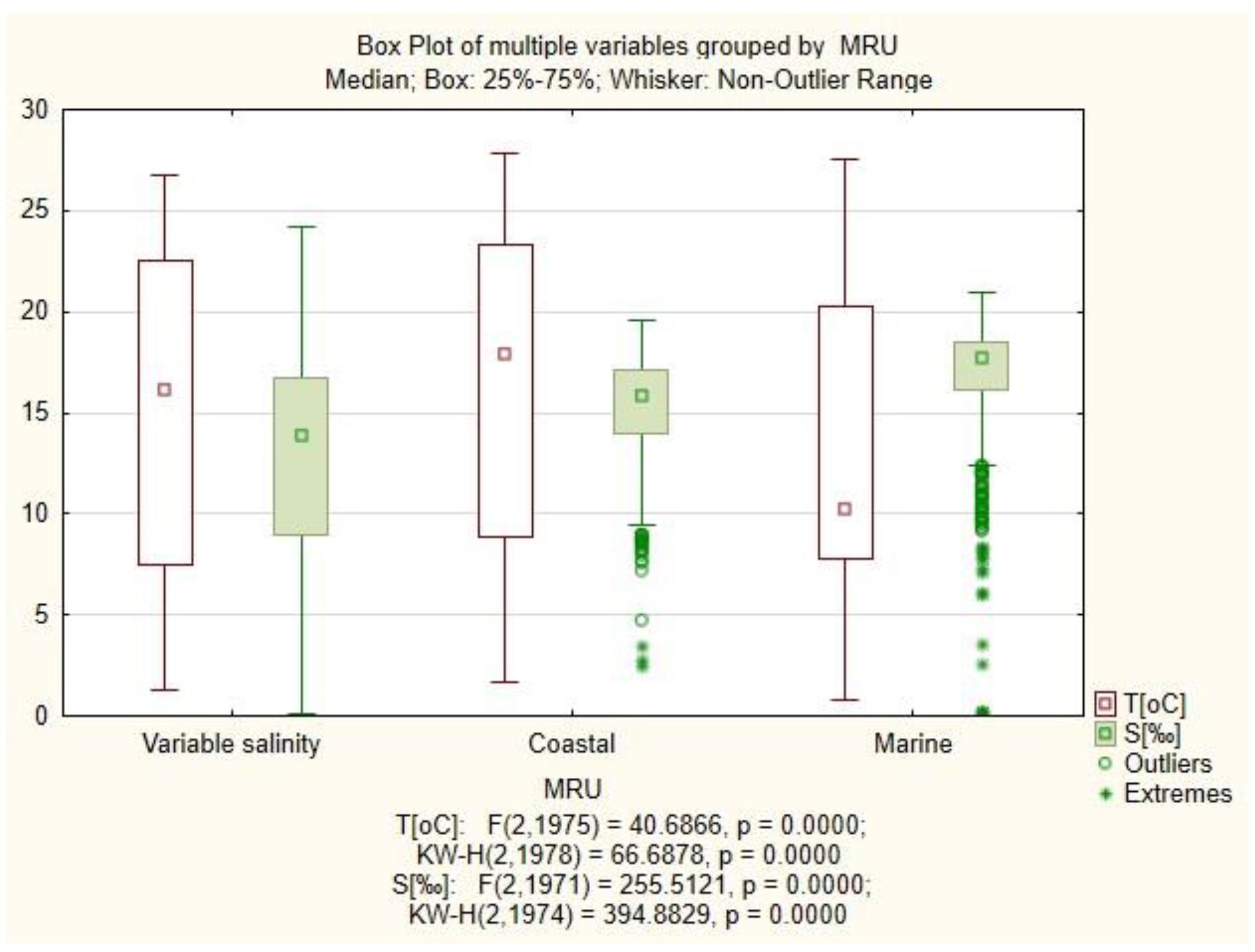
3.1. Physicochemical Factors

The general physicochemical parameters and nutrient levels exhibited considerable variability due to the extensive spatiotemporal distribution (Table S2). There were notable temporal trends, with both temperature and salinity showing significant increases over time, growing at rates of 0.1 °C/year and 0.28‰/year, respectively (Figure 2 and Figure 3).
In terms of spatial distribution, the temperature gradient underscores a decline from north to south, mirroring the overall pattern of sea currents. Conversely, salinity exhibits an opposite trend, decreasing from shore to the shelf in marine waters (Figure 4). Dissolved nutrient concentrations show no significant temporal fluctuations; however, their spatial distribution varies notably. The highest values are observed in regions directly influenced by the Danube, followed by the coastal area and shelf marine waters (Figure 5 and Figure 6). There are significant differences in environmental parameters among MRUs. In summary, ANOVA results show that the environmental parameters (t, S, nutrient concentrations) significantly vary among different MRUs (Figure 4, Figure 5 and Figure 6).

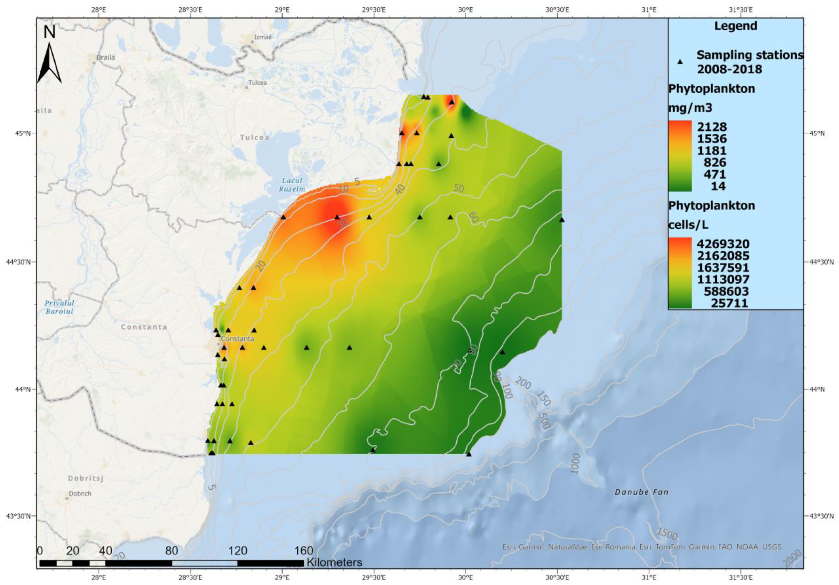
3.2. Phytoplankton Spatial Distribution in 2008–2018

Within the phytoplankton community, a total of 347 species belonging to 16 classes were identified. Bacillariphyceae, Dinophyceae, Chlorophyceae, and Cyanophyceae were the most diverse classes. The diatoms (Bacillaryophyceae) reached their highest proportions during March and April (43%, respectively, 38%), and then decreased to 23–34% during the warmer months (May–September). During June, July, and August, a higher diversity of the dinoflagellates (30–37% of the total) could be observed. The chlorophyte (Chlorophyceae) and cyanobacteria (Cyanophyceae) proportions in the qualitative structure of the phytoplankton also increased during the warmer months, beginning with May (up to 17% and 11%, respectively) (Figure 7).
The phytoplankton distribution map shows that the highest values were recorded in waters with variable salinity (the stations under the influence of the Danube’s mouths), but also in the coastal waters near Constanta harbor and the marine waters of Mangalia profiles (Table S3 and Figure 8). According to one-way ANOVA, the p-value was less than 0.05 for both phytoplankton density and biomass, suggesting significant differences among marine reporting units (Table S4).

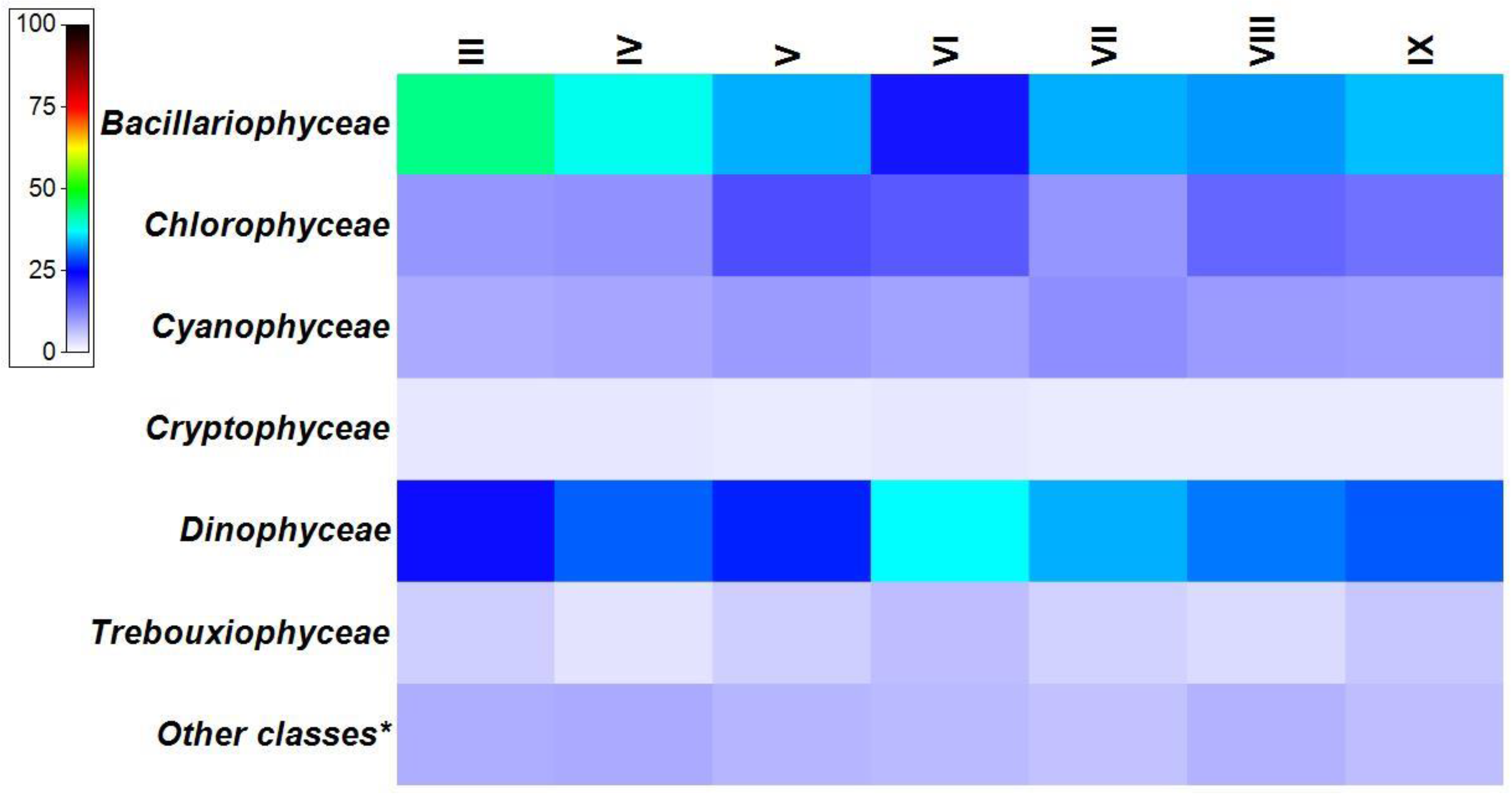
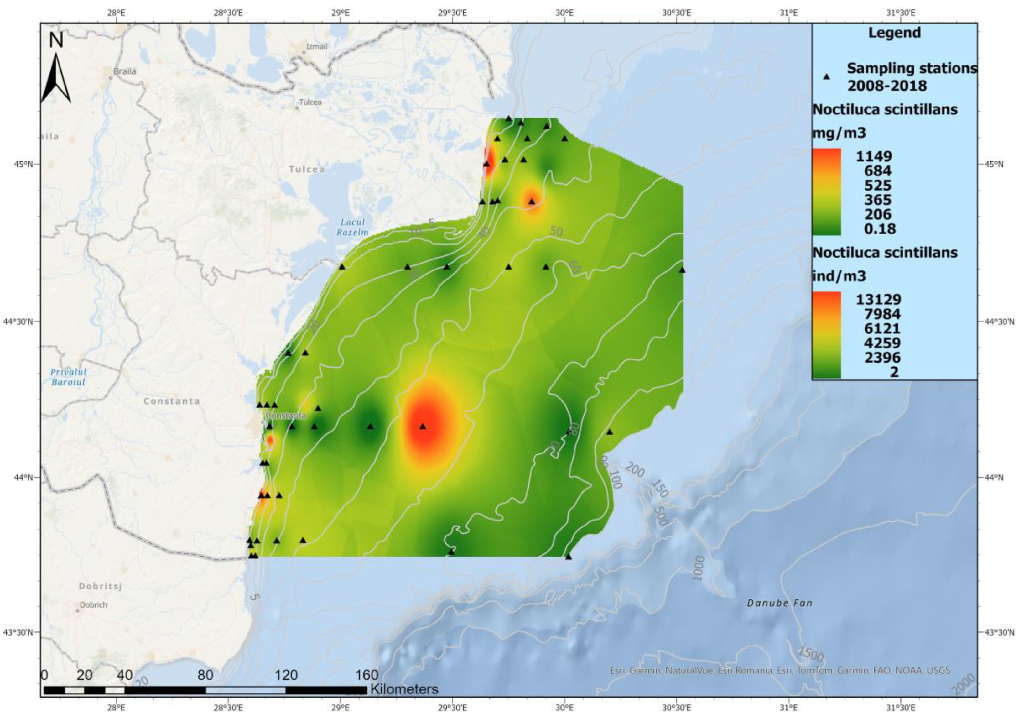
3.3. Zooplankton Spatial Distribution in 2008–2018

In order to analyze the zooplankton community of the Romanian Black Sea, we separated the fodder component, which comprised copepods, cladocerans, meroplankton, and “other groups”, from the nonfodder zooplankton, represented by Noctiluca scintillans. The latter, due to its large cell size (>200 μm) and phagotrophic feeding behavior, was assessed within the zooplankton community [48]. There were variations for N. scintillans, which was found to be less prevalent in coastal waters but to have high density and biomass values in marine waters and waters with variable salinity (Table S3 and Figure 9). The dynamics of N. scintillans are complex and depends on many factors, which can differ among locations [49]. Numerous studies have identified a range of factors associated with the densities of N. scintillans. These factors include eutrophication and specific nutrients, particularly phosphate; chlorophyll a; the presence of other plankton species such as diatom spring blooms; and zooplankton biomass [49,50,51,52]. Additionally, the physical characteristics of the water column, such as winter sea surface temperature, have been found to correlate with N. scintillans densities. Furthermore, weather conditions, including factors like rainfall and wind direction, have also been identified as influential in understanding the variations in N. scintillans populations [49,53,54].
Coastal waters displayed the most significant presence of fodder zooplankton (Table S3 and Figure 10), with copepods, cladocerans, and meroplanktonic elements constituting the bulk of the community (Figure 11). The ANOVA results show that biological parameters (zooplankton density and biomass) significantly vary among different MRUs (Table S4).

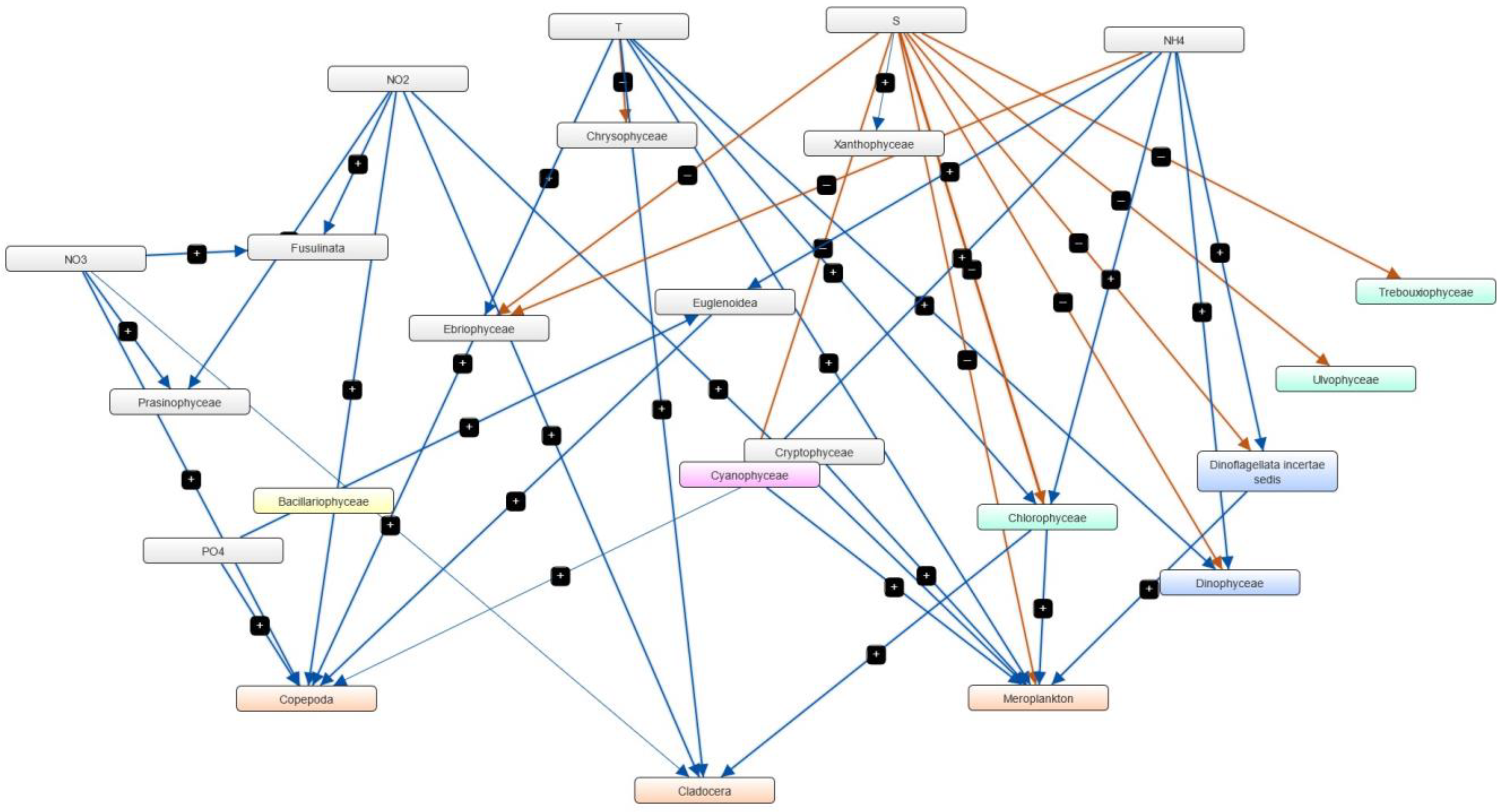
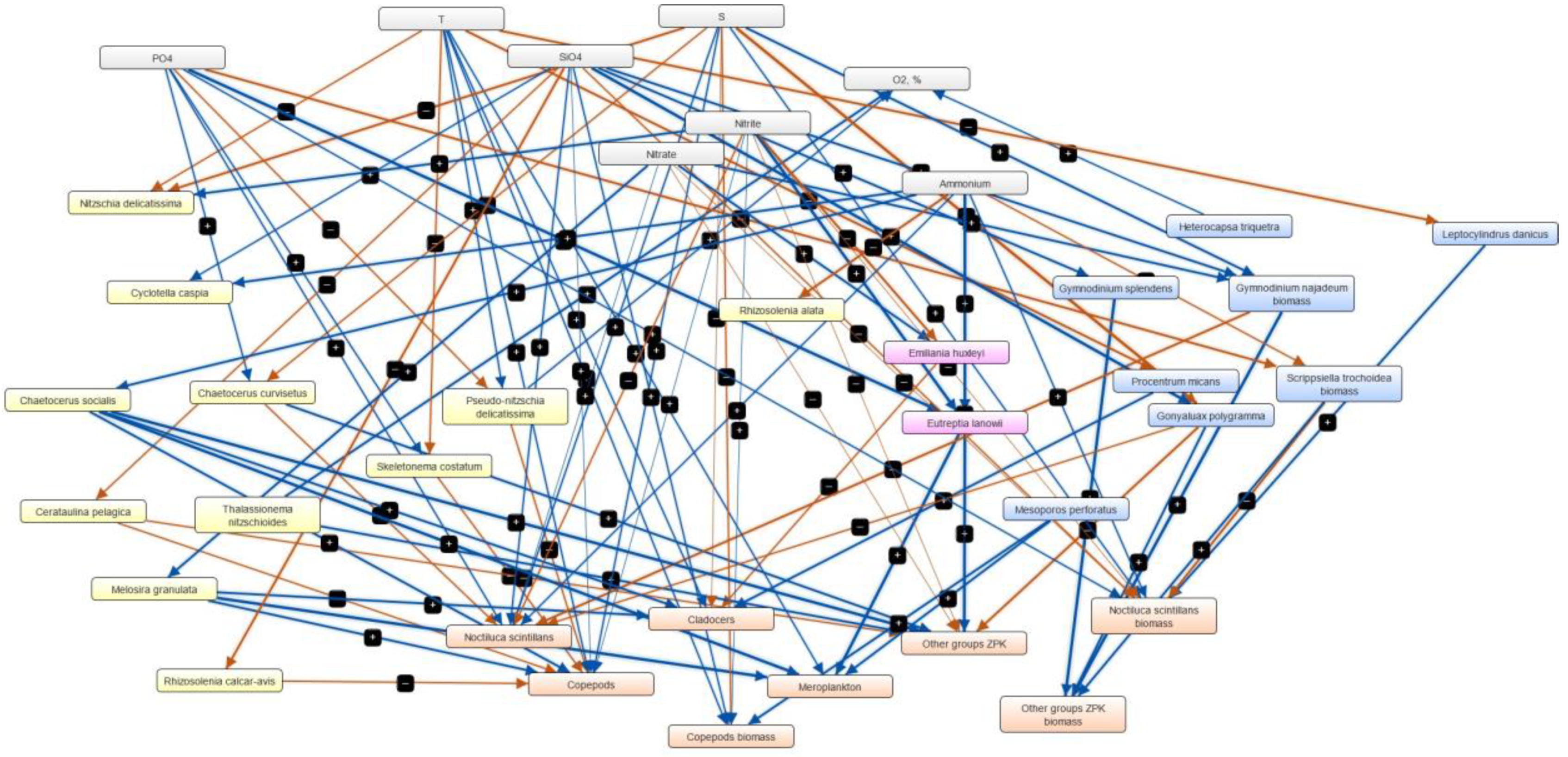
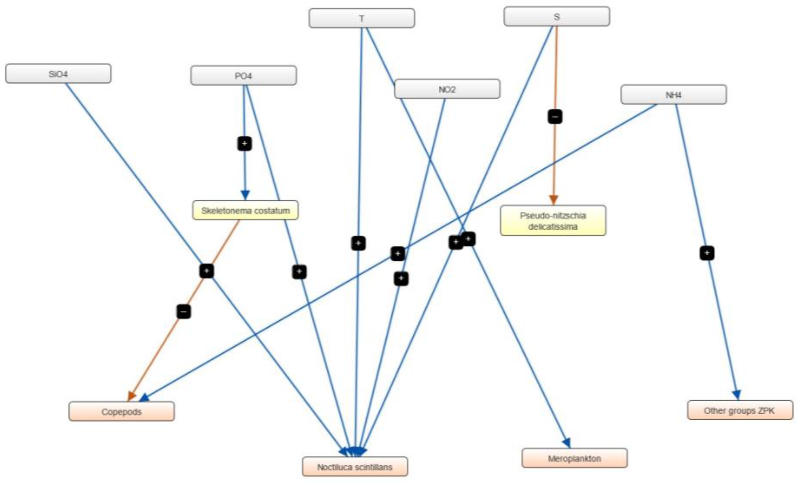
3.4. Semi-Quantitative Models of the Causal Relationships between Phytoplankton, Zooplankton and Physico-Chemical Parameters

Semi-quantitative models, illustrating the causal relationships between phytoplankton, zooplankton, and physicochemical parameters, were constructed through the application of statistical analysis and the Mental Modeler software. The data entered into the model (Table 1) included significant (p < 0.05) correlation coefficients and these were used to determine the physico-chemical parameters with phytoplankton, phytoplankton–zooplankton, and zooplankton linkages. These connections are organized based on various variables, such as marine reporting units, class, and specific phytoplankton species.
Thus, in waters with variable salinity under the direct influence of the Danube, temperature reduction favors the development of diatoms (r = −0.39) and copepods (r = −0.23). In addition to positively influencing the development of cladocerans (r = 0.28), the development of dinoflagellates is favored by rising temperatures (r = 0.24) and lower PO4 (r = −0.35). The development of species belonging to the Chlorophyceae class is favored by an increase in temperature (r = 0.27) and NH4 concentration (r = 0.26) and a decrease in salinity (r = −0.35) and PO4 (r = −0.35). Temperature improves the development of species in the Cyanophyceae class (r = 0.27), which in turn has a good effect on the growth of copepods (r = 0.37) and meroplankton (r = 0.21) (Figure 12 and Table S5).
In coastal waters, the following patterns were observed: the increase in NH4 and NO2 concentrations favored the formation of diatoms (r = 0.27). At the same time, rising temperature (r = 0.27), lower salinity (r = −0.2), and high NH4 concentration (r = 0.22) promoted the growth of dinoflagellates. Low salinity (r = −0.5), rising temperature (r = 0.27), and a high NH4 concentration (r = 0.28) promoted the development of species belonging to the Chlorophyceae class. All these factors also had a beneficial impacts on the development of meroplankton (r = 0.18) and cladocerans (r = 0.31). The NH4 concentration (r = 0.2) and salinity (r = −0.45) had an impact on species belonging to the Cyanophyceae class, and they also had a favorable effect on meroplankton development (r = 0.2) (Figure 13 and Table S6).
In marine shelf waters at a distance from the shore, the growth of diatoms was stimulated by a drop in salinity (r = −0.32) and temperature (r = −0.17), as well as by an increase in PO4 concentration (r = 0.32). The latter had an adverse effect on copepod development (r = −0.18). On the other hand, increasing temperature (r = 0.36), NH4 concentration (r = 0.27), and decreasing salinity (r = −0.17) were favorable for dinoflagellate and copepod development (r = 0.16). The rise in PO4 (r = 0.2) and NH4 (r = 0.17) concentrations, as well as the fall in salinity (r = −0.35), promoted the development of species belonging to the Chlorophyceae class, while the drop in salinity had a positive impact on the species in the Cyanophyceae class (r = −0.19) (Figure 14 and Table S7).
The outcomes of the phytoplankton growth models show that, at normal densities, salinity, phosphate, silicate, and ammonium concentrations considerably impact the species Chaetoceros socialis. When the diatom C. socialis is present in amounts of less than 106 cells/L, it promotes zooplankton growth, while blooms surpassing 106 cells/L have an adverse effect on copepod development (Figure 15).
Eutreptia lanowii is the primary component in the model of abundant growth up to 106 cells/L because of its robust correlations with nutrients (phosphates, nitrates, and ammonium) and with “other groups” (Figure 16). While it was previously uncommon or nonexistent in Romanian coastal waters, it became common between 1976 and 1977 due to high nutrient concentrations [55].
Skeletonema costatum and N. scintillans have been identified as the prevailing species of bloom. Thus, the pelagic habitat’s condition is influenced by abiotic variables such as temperature, phosphates, and salinity, causing disturbances (Figure 17).

4. Discussion

The current study found that, while the average temperature significantly increased during the study period, there were distinct correlations between temperature and the presence of phytoplankton and zooplankton, indicating that seawater warming has wide-ranging effects on marine plankton. It has been noted in the literature that the abundance of phytoplankton and zooplankton is influenced by various factors, including climatic, hydrological, biological, geological, and anthropogenic elements [56,57,58]. Additionally, both physical and chemical variables are significant contributors to the composition, diversity, and abundance of species [59,60,61], including marine organisms such as plankton [57,62]. Studies have shown that changes in the composition and abundance of phytoplankton and zooplankton communities are linked to fluctuations in environmental factors due to seasonality [63,64,65,66]. In our current research, both phytoplankton and zooplankton exhibited quantitative variations according to seasonal patterns. During the summer season, their abundances and biomasses were observed to be higher compared to those in the spring season (Table S3).
Thus, warming changes the composition of the phytoplankton community by promoting dinoflagellates, which can mean fewer food sources for zooplankton [67]. Also, warmer temperatures can increase the basal metabolic rates of zooplankton. However, they can also increase respiratory demand, which reduces their aerobic range of motion and leaves them with less energy for growth and reproduction [68]. Lastly, a partial explanation for the decrease in zooplankton in warmer temperatures can be found in the disturbance of zooplankton’s overwintering strategies [69].
Changes in salinity have an impact on photosynthetic rates, especially for some phytoplankton groups which can only exist in narrow salinity ranges [70]. In the present study, species belonging to the Clorophyceae and Cyanophyceae classes had significant negative correlations with salinity. Several studies have reported the dominance of Chlorophyceae and Cyanophyceae in estuarine ecosystems dominated by freshwater inputs [71,72].
It is well recognized that salinity is a powerful driver of change in the zooplankton community [3]: a rise in salinity alters zooplankton composition and abundance [35]. In this study, copepods and cladocerans had a significant positive correlation with salinity, showing their preference for higher salinity. High-salinity-tolerant zooplankton progressively select out species with low salinity tolerance and thrive and reproduce quickly as salinity rises, with zooplankton responding differently to varying salinity concentrations [73].
The temporal and spatial variability of nutrient availability controlled the phytoplankton population composition and distribution. Thus, while high nutrient levels promoted phytoplankton proliferation, low nutrient concentrations close to the cell surface restricted nutrient uptake, which had an impact on biomass yield (Liebig’s Law) and growth rate (Blakman rate limit) [74].
The results obtained using FCM revealed that phytoplankton can suppress copepods’ development. This mainly occurs in waters with variable salinity and marine shelf waters because diatom development leads to a reduction in copepods, which happens mainly at lower temperatures and when salinity occurs. Other studies have shown that diatoms block the embryonic development of copepods [75]. Diatoms interfere with copepod embryogenesis and induce strong developmental aberrations in nauplii development stages. Evidence of diatoms’ inhibitory effect on copepods was also reported by several authors, who found that hatching success in copepods was modified after diatom blooms [75] by synthesizing hydroxy-fatty acids (HFA) and their derivatives, which have teratogenic as well as hatching and growth-inhibiting properties [76].
Large diatoms, commonly referred to as “storage specialists”, are also noted for their exceptional efficiency in absorbing and storing available nutrients in vacuoles [77], as shown in the present study, where the increase in NH4 and NO2 concentrations in coastal waters favored the formation of large diatoms. Compared to small cells, whose relative abundance tends to decline with increased nutrient availability, large-celled phytoplankton tend to become more common and dominate under high nutritional circumstances [78,79].
On the other hand, when mainly feeding on phytoplankton, copepods can modify the dynamics of phytoplankton [68,69,70,80,81]. Copepods are the predominant zooplankton species in most marine water bodies worldwide [80,81] and they are crucial in transferring carbon from phytoplankton to species at higher trophic levels, including fish and marine mammals [82].
In our study, an increase in temperature showed better development for species belonging to the Cyanophyceae class in waters with variable salinity, promoting copepod and meroplankton development. On the other hand, other studies showed that cyanobacteria had neutral or positive effects on zooplankton egg production, hatching, and juvenile development due to complimentary nutrients and microelements, e.g., amino acids, antioxidants, vitamins, proteins, phosphorus, and nitrogen [83,84,85,86]. Offering particular value for copepods, summer blooms of diazotrophic filamentous cyanobacteria could be essential for their growth and reproduction, providing complementary food, supporting high antioxidant levels, and fueling the growth of microbial prey [87]. The populations of zooplankton that cooccur with dense cyanobacterial populations may be better able than unexposed zooplankton to digest cyanobacteria [88].
In coastal waters, NH4 and salinity impact species belonging to the Cyanophyceae class, and they also have a favorable effect on meroplankton development [89]. Several studies have stated that the size distribution of organisms and the coupling between primary and secondary producers are also highly influenced by input frequency and seasonality [52,53]. An abundant food supply for planktotrophic larvae can lead to indirect induction through the control of both the phytoplankton blooms and gamete, larval release by the physical environment, or direct induction, with the increasing phytoplankton abundance acting as a chemical triggering cue for spawning [90,91].
The seasonal reproductive pulse can boost interspecies competition and decrease an individual’s predation risk [92]. According to several studies [93,94], many benthic species have a single prominent hatching peak that coincides with warmer water temperatures, implying shorter developmental times, or with spring phytoplankton blooms, involving greater food availability and diminished competition [90].
Being an inland water body, the Black Sea is highly susceptible to changes in the surrounding environment. It has been dramatically impacted over several decades by many phenomena, including invasive species introduction, eutrophication, climate change, and overfishing [95]. Toxic blooms of diatoms and dinoflagellates occur relatively frequently in the NW Black Sea along the coasts of Romania and Bulgaria [95,96,97,98,99,100,101,102]. This was seen in the present study, where the dominant species in phytoplankton blooms were the diatom S. costatum and the dinoflagellate N. scintillans.
Consequently, complex environmental factors and their combination, including light availability, nutrient supply, vertical mixing rate, grazing pressure, and meteorological conditions, affect blooms, while they vary depending on the oceanographic conditions of a given region [99,100,102,103].
Fuzzy cognitive mapping, a soft system methodology capable of semi-quantifying qualitative data, was already being used in the Romanian Black Sea area, resulting in the production of several scientific articles [104,105,106]. The findings suggest that certain significant concepts play crucial roles in the perceived resilience of the Black Sea and its attainment of a good environmental state. The resultant fuzzy model offers the capability to analyze, simulate, and assess the impact of parameters, thereby predicting the behavior of a system. Semi-quantitative models provide unique approaches for studying the state of the Black Sea and the combined effects of different parameters on its condition. They have the potential to serve as decision-making tools for assessing various scenarios.

5. Conclusions

Although the structure of biological communities in all marine habitats is mainly determined by the interaction of physical and biological processes, it is important to understand the intricacy of this interaction at all scales. The distribution patterns of planktonic organisms offer a conceptual framework for the evaluation of the different variables that produce and sustain those patterns; therefore, knowledge of basic processes and the integration of models are necessary for forecasting and comprehending the functioning of ecosystems.
In order to preserve the Black Sea’s natural biodiversity, phytoplankton must be monitored. This is for the purpose of accurately identifying and diagnosing the “plankton bloom” brought on by the development of potentially toxic species. The growing coastal pressures from anthropogenic activities pose severe problems for these algae; hence it is important to monitor their levels. Time-series analysis is an exclusive technique used for evaluating changes and patterns linked to regional impacts, experimenting with theories about phytoplankton ecology, and offering a consistent image of the yearly cycle of phytoplankton populations, as well as the interactions with other biotic and abiotic elements.
This study establishes a foundation for understanding the complex interactions between abiotic variables and pelagic habitat components. It may help to create forecasting models and support policy decisions about the management of nutrient releases and other factors that stimulate the growth of harmful algae, particularly in the era of climate change. The results can also help in the preparation of policies and management activities by showing specific alterations that might harm aquatic environments.

Supplementary Materials

The following supporting information can be downloaded at: https://www.mdpi.com/article/10.3390/phycology4010010/s1, Table S1. Sample size for each season and marine reporting unit, Table S2. Descriptive statistics of physicochemical parameters and dissolved nutrients in Black Sea waters (2008–2018), Table S3. Phytoplankton and zooplankton abundances and biomasses for each marine reporting unit and season, Table S4. One-way ANOVA for Biological parameters grouped by MRU (calculated with STATISTICA), Table S5. Correlations between biological and environmental parameters in FCM, waters with variable salinity, Table S6. Correlations between biological and environmental parameters in FCM, coastal waters, Table S7. Correlations between biological and environmental parameters in FCM, marine waters.

Author Contributions

Conceptualisation, E.B., L.L. and O.V.; methodology, E.B., L.L. and O.V.; software, E.B., L.L. and O.V.; validation, E.B., L.L. and O.V.; formal analysis, E.B., L.L. and O.V.; investigation, E.B., L.L. and O.V.; resources, E.B., L.B., E.P., F.T., L.L. and O.V.; data curation, E.B., L.B., E.P., F.T., L.L. and O.V.; writing—original draft preparation, E.B., L.L. and O.V.; writing—review and editing, E.B., E.P., L.L. and O.V.; visualisation, E.B., L.B., E.P., F.T., L.L. and O.V.; supervision, E.B, L.L. and O.V.; project administration, E.B., L.L. and O.V.; funding acquisition, E.B. All authors have read and agreed to the published version of the manuscript.

Funding

This research was funded by the Nucleu Programme INTELMAR 2019–2022 funded by Ministry of Research, Innovation, and Digitization, grant number 45N/2019, project PN 19260202, and by Nucleu Programme SMART-BLUE 2023-2026 funded by Ministry of Research, Innovation, and Digitization, grant number 33N/2023, PN23230201 and PN23230103.

Institutional Review Board Statement

Not applicable.

Informed Consent Statement

Not applicable.

Data Availability Statement

The data belong to the National Institute for Marine Research and Development “Grigore Antipa” (NIMRD) and can be accessed by request to http://www.nodc.ro/data_policy_nimrd.php (accessed on 15 January 2024).

Conflicts of Interest

The authors declare no conflicts of interest. The funders had no role in the de-sign of the study; in the collection, analyses, or interpretation of data; in the writing of the manuscript; or in the decision to publish the results.

References

  1. Irigoien, X.; Huisman, J.; Harris, R.P. Global Biodiversity Patterns of Marine Phytoplankton and Zooplankton. Nature 2004, 429, 863–867. [Google Scholar] [CrossRef] [PubMed]
  2. DeLong, E.F.; Karl, D.M. Genomic Perspectives in Microbial Oceanography. Nature 2005, 437, 336–342. [Google Scholar] [CrossRef] [PubMed]
  3. Wei, Y.; Ding, D.; Gu, T.; Jiang, T.; Qu, K.; Sun, J.; Cui, Z. Different Responses of Phytoplankton and Zooplankton Communities to Current Changing Coastal Environments. Environ. Res. 2022, 215, 114426. [Google Scholar] [CrossRef]
  4. Jakhar, P. Role of Phytoplankton and Zooplankton as Health Indicators of Aquatic Ecosystem: A Review. Int. J. Innov. Res. Sci. Stud. 2013, 2, 489–500. [Google Scholar]
  5. Onyema, I.C.; Lawal-Are, A.O.; Bassey, T.A.; Bassey, O.B. Water Quality Parameters, Chlorophyll a and Zooplankton of an Estuarine Creek in Lagos. J. Am. Sci. 2009, 5, 76–94. [Google Scholar]
  6. Hays, G.; Richardson, A.; Robinson, C. Climate Change and Marine Plankton. Trends Ecol. Evol. 2005, 20, 337–344. [Google Scholar] [CrossRef]
  7. Barton, A.D.; Irwin, A.J.; Finkel, Z.V.; Stock, C.A. Anthropogenic Climate Change Drives Shift and Shuffle in North Atlantic Phytoplankton Communities. Proc. Natl. Acad. Sci. USA 2016, 113, 2964–2969. [Google Scholar] [CrossRef] [PubMed]
  8. Edwards, M.; Richardson, A.J. Impact of Climate Change on Marine Pelagic Phenology and Trophic Mismatch. Nature 2004, 430, 881–884. [Google Scholar] [CrossRef]
  9. Lv, Y.; Pei, Y.; Gao, S.; Li, C. Harvesting of a Phytoplankton-Zooplankton Model. Nonlinear Anal. Real World Appl. 2010, 11, 3608–3619. [Google Scholar] [CrossRef]
  10. Guy, D. The Ecology of the Fish Pond Ecosystem with Special Reference to Africa; Pergamon Press: Oxford, UK, 1992; pp. 220–230. [Google Scholar]
  11. Tas, B.; Gonulol, A. An Ecologic and Taxonomic Study on Phytoplankton of a Shallow Lake, Turkey. J. Environ. Biol. 2007, 28, 439–445. [Google Scholar]
  12. Contreras, J.J.; Sarma, S.S.S.; Merino-Ibarra, M.; Nandini, S. Seasonal Changes in the Rotifer (Rotifera) Diversity from a Tropical High Altitude Reservoir (Valle de Bravo, Mexico). J. Environ. Biol. 2009, 30, 191–195. [Google Scholar] [PubMed]
  13. Chandran, R.; Jaiswar, A.K.; Raizada, S.; Mandal, S.; Mayekar, T.S.; Bisht, A.S.; Singh, S.K.; Mohindra, V.; Lal, K.K.; Tyagi, L.K. Plankton Dynamics and Their Relationship with Environmental Factors Shape Fish Community Structure in Fluvial Ecosystem: A Case Study. Indian J. Fish. 2021, 68, 1–13. [Google Scholar] [CrossRef]
  14. Gray, S.; Zanre, E.; Gray, S. Fuzzy Cognitive Maps as Representations of Mental Models and Group Beliefs. In Fuzzy Cognitive Maps for Applied Sciences and Engineering: From Fundamentals to Extensions and Learning Algorithms; Springer: Berlin/Heidelberg, Germany, 2013; pp. 29–48. [Google Scholar]
  15. Fonseca, K.; Espitia, E.; Breuer, L.; Correa, A. Using Fuzzy Cognitive Maps to Promote Nature-Based Solutions for Water Quality Improvement in Developing-Country Communities. J. Clean. Prod. 2022, 377, 134246. [Google Scholar] [CrossRef]
  16. Uusitalo, L.; Jernberg, S.; Korn, P.; Puntila-Dodd, R.; Skyttä, A.; Vikström, S. Fuzzy Cognitive Mapping of Baltic Archipelago Sea Food Webs Reveals No Cliqued Views of the System Structure between Stakeholder Groups. Socio-Environ. Syst. Model. 2020, 2, 16343. [Google Scholar] [CrossRef]
  17. Stier, A.C.; Samhouri, J.F.; Gray, S.; Martone, R.G.; Mach, M.E.; Halpern, B.S.; Kappel, C.V.; Scarborough, C.; Levin, P.S. Integrating Expert Perceptions into Food Web Conservation and Management. Conserv. Lett. 2017, 10, 67–76. [Google Scholar] [CrossRef]
  18. Jetter, A.J.; Kok, K. Fuzzy Cognitive Maps for Futures Studies—A Methodological Assessment of Concepts and Methods. Futures 2014, 61, 45–57. [Google Scholar] [CrossRef]
  19. Özesmi, U.; Özesmi, S.L. Ecological Models Based on People’s Knowledge: A Multi-Step Fuzzy Cognitive Mapping Approach. Ecol. Model. 2004, 176, 43–64. [Google Scholar] [CrossRef]
  20. Gray, S.A.; Gray, S.; Cox, L.J.; Henly-Shepard, S. Mental Modeler: A Fuzzy-Logic Cognitive Mapping Modeling Tool for Adaptive Environmental Management. In Proceedings of the 2013 46th Hawaii International Conference on System Sciences, Wailea, HI, USA, 7–10 January 2013; pp. 965–973. [Google Scholar]
  21. Stanev, E.V.; Peneva, E.; Chtirkova, B. Climate Change and Regional Ocean Water Mass Disappearance: Case of the Black Sea. J. Geophys. Res. Ocean. 2019, 124, 4803–4819. [Google Scholar] [CrossRef]
  22. Magliozzi, C.; Palma, M.; Druon, J.-N.; Palialexis, A.; Abigail, M.-G.; Ioanna, V.; Rafael, G.-Q.; Elena, G.; Birgit, H.; Laura, B.; et al. Status of Pelagic Habitats within the EU-Marine Strategy Framework Directive: Proposals for Improving Consistency and Representativeness of the Assessment. Mar. Policy 2023, 148, 105467. [Google Scholar] [CrossRef]
  23. Oguz, T. (Ed.) State of the Environment of the Black Sea (2001-2006/7); Publications of the Commission on the Protection of the Black Sea Against Pollution (BSC): Istanbul, Turkey, 2008. [Google Scholar]
  24. Konovalov, S.K.; Murray, J.W. Variations in the Chemistry of the Black Sea on a Time Scale of ž/Decades 1960–1995. J. Mar. Syst. 2001, 31, 217–243. [Google Scholar] [CrossRef]
  25. Nedelcu, L.-I.; Tanase, V.-M.; Rusu, E. An Evaluation of the Wind Energy along the Romanian Black Sea Coast. Inventions 2023, 8, 48. [Google Scholar] [CrossRef]
  26. Mihailov, M.E.; Tomescu-Chivu, M.I.; Dima, V. Black Sea Water Dynamics on the Romanian Littoral—Case Study: The Upwelling Phenomena. Rom. Rep. Phys. 2012, 64, 232–245. [Google Scholar]
  27. Lazăr, L. (Ed.) Anthropogenic Pressures and Impacts on the Black Sea Coastal Ecosystem; CD Press: Constanta, Romania, 2021. [Google Scholar]
  28. Lazăr, L. (Ed.) Impact of the Rivers on the Black Sea Ecosystem; CD Press: Constanta, Romania, 2021. [Google Scholar]
  29. Moncheva, S.; Parr, B. Manual for Phytoplankton Sampling and Analysis in the Black Sea; Black Sea Commission: Istanbul, Turkey, 2010. [Google Scholar]
  30. Kisselew, I.A. Dinoflagellata; Fauna URSS: Moscova, Russia, 1950. [Google Scholar]
  31. Proshkina-Lavrenko, A.I. (Ed.) Planktonic Diatoms from the Black Sea; Fauna URSS: Moscova, Russia, 1995. [Google Scholar]
  32. Carmelo, R.T. (Ed.) Identifying Marine Diatoms and Dinoflagellataes; Academic Press: Cambridge, MA, USA, 1995. [Google Scholar]
  33. Schiller, J. (Ed.) Dinoflagellatae, Rabenhorst’s Cryptogamen—Flora Leipzig II; Akademische Verlagsgesellschaft M. B. H.: Leipzig, Germany, 1937. [Google Scholar]
  34. Moncheva, S.; Doncheva, V.; Boicenco, L.; Sahin, F.; Slabakova, N.; Culcea, O. Report on the MISIS Cruise Intercalibration Exercise: Phytoplankton; Ex. Ponto: Constanta, Romania, 2014. [Google Scholar]
  35. Hutchinson, G.E. (Ed.) A Treatise on Limnology. In Introduction to Lake Biology and the Limnoplankton; J. Wiley & Sons: New York, NY, USA, 1967; Volume 2. [Google Scholar]
  36. Alexandrov, B.; Arashkevich, E.; Gubanova, A.; Korshenko, A. Manual for Mesozooplankton Sampling and Analysis in the Black Sea Monitoring; Black Sea Commission: Istanbul, Turkey, 2014. [Google Scholar]
  37. Mordukhay-Boltovskoy, F.D. (Ed.) Identification Manual on the Fauna of the Black and Azov Seas; Naukova Dumka Pub: Kiev, Ukraine, 1968. [Google Scholar]
  38. Mordukhay-Boltovskoy, F.D. (Ed.) Guide of the Black Sea and the Sea of Azov Fauna; Naukova Dumka Pub: Kiev, Ukraine, 1972. [Google Scholar]
  39. Petipa, T.S. On the Mean Weight of the Principle Forms of Zooplankton in the Black Sea. Sevast. Biol. Station 1957, 9, 39–57. [Google Scholar]
  40. Grasshoff, K.; Kremling, K.; Ehrhardt, M. (Eds.) Methods of Seawater Analysis; Willey-VCH: Weinheim, Germany, 1999. [Google Scholar]
  41. Mullin, J.B.; Riley, J.P. The Spectrophotometric Determination of Nitrate in Natural Waters, with Particular Reference to Sea-Water. Anal. Chim. Acta 1955, 12, 464–480. [Google Scholar] [CrossRef]
  42. Clarke, K.R.; Warwick, R.M. Change in Marine Communities: An Approach to Statistical Analysis, 3rd ed.; PRIMER-E: Plymouth, UK, 2014. [Google Scholar]
  43. Addinsoft, Inc. Addinsoft XLSTAT Software; Version 2021.2.1; Addinsoft, Inc.: New York, NY, USA, 2021. [Google Scholar]
  44. TIBCO Software, Inc. TIBCO Statistica; Version 14.0.1.25; TIBCO Software, Inc.: Palo Alto, CA, USA, 2023. [Google Scholar]
  45. ESRI. ArcGIS Desktop; Version 10.7; Environmental Systems Research Institute: Redlands, CA, USA, 2019. [Google Scholar]
  46. Al-Mamoori, S.K.; Al-Maliki, L.A.; Al-Sulttani, A.H.; El-Tawil, K.; Al-Ansari, N. Statistical Analysis of the Best GIS Interpolation Method for Bearing Capacity Estimation in An-Najaf City, Iraq. Environ. Earth Sci. 2021, 80, 683. [Google Scholar] [CrossRef]
  47. Putra, M.; Lewis, S.; Kurniasih, E.; Prabuning, D.; Faiqoh, E. Plankton Biomass Models Based on GIS and Remote Sensing Technique for Predicting Marine Megafauna Hotspots in the Solor Waters. IOP Conf. Ser. Earth Environ. Sci. 2016, 47, 012015. [Google Scholar] [CrossRef]
  48. Aytan, U.; Senturk, Y. Dynamics of Noctiluca Scintillans (Macartney) Kofoid & Swezy and Its Contribution to Mesozooplankton in the Southeastern Black Sea. Aquat. Sci. Eng. 2018, 33, 84–89. [Google Scholar] [CrossRef]
  49. Ollevier, A.; Mortelmans, J.; Aubert, A.; Deneudt, K.; Vandegehuchte, M.B. Noctiluca Scintillans: Dynamics, Size Measurements and Relationships with Small Soft-Bodied Plankton in the Belgian Part of the North Sea. Front. Mar. Sci. 2021, 8, 777999. [Google Scholar] [CrossRef]
  50. Fonda Umani, S. Noctiluca Scintillans MACARTNEY in the Northern Adriatic Sea: Long-Term Dynamics, Relationships with Temperature and Eutrophication, and Role in the Food Web. J. Plankton Res. 2004, 26, 545–561. [Google Scholar] [CrossRef]
  51. Elbrächter, M.; Qi, Z. Aspects of Noctiluca (Dinophyceae) Population Dynamics. In Physiological Ecology of Harmful Algal Blooms; Anderson, D.M., Cembella, A.D., Hallegraeff, G.M., Eds.; Springer: Berlin/Heidelberg, Germany, 1998. [Google Scholar]
  52. Turkoglu, M. Red Tides of the Dinoflagellate Noctiluca Scintillans Associated with Eutrophication in the Sea of Marmara (the Dardanelles, Turkey). Oceanologia 2013, 55, 709–732. [Google Scholar] [CrossRef]
  53. Miyaguchi, H.; Fujiki, T.; Kikuchi, T.; Kuwahara, V.S.; Toda, T. Relationship between the Bloom of Noctiluca Scintillans and Environmental Factors in the Coastal Waters of Sagami Bay, Japan. J. Plankton Res. 2006, 28, 313–324. [Google Scholar] [CrossRef]
  54. Nakamura, Y. Biomass, Feeding and Production of Noctiluca Scintillans in the Seto Inland Sea, Japan. J. Plankton Res. 1998, 20, 2213–2222. [Google Scholar] [CrossRef]
  55. Mihnea, P.E. Qualitative and Quantitative Aspects of the Alga Eutreptia Lanowii (Steuer) in Relation to the Coastal Pollution Phenomenon. Cercet. Mar. Rech. Mar. 1978, 11, 225–233. [Google Scholar]
  56. Bartram, J.; Balance, R. (Eds.) Water Quality Monitoring: A Practical Guide to the Design Implementation of Freshwater Quality Studies and Monitoring Programmes; TJ Press: London, UK, 1996. [Google Scholar]
  57. Gogoi, P.; Sinha, A.; Das Sarkar, S.; Chanu, T.N.; Yadav, A.K.; Koushlesh, S.K.; Borah, S.; Das, S.K.; Das, B.K. Seasonal Influence of Physicochemical Parameters on Phytoplankton Diversity and Assemblage Pattern in Kailash Khal, a Tropical Wetland, Sundarbans, India. Appl. Water Sci. 2019, 9, 156. [Google Scholar] [CrossRef]
  58. Stelmakh, L.; Kovrigina, N.; Gorbunova, T. Phytoplankton Seasonal Dynamics under Conditions of Climate Change and Anthropogenic Pollution in the Western Coastal Waters of the Black Sea (Sevastopol Region). J. Mar. Sci. Eng. 2023, 11, 569. [Google Scholar] [CrossRef]
  59. Ahmad, U.; Parveen, S.; Khan, A.A.; Kabir, H.A.; Mola, H.R.A.; Ganai, A.H. Zooplankton Population in Relation to Physico-Chemical Factors of a Sewage Fed Pond of Aligarh (UP), India. Biol. Med. 2011, 3, 336–341. [Google Scholar]
  60. Limbu, S.M.; Kyewalyanga, M.S. Spatial and Temporal Variations in Environmental Variables in Relation to Phytoplankton Composition and Biomass in Coral Reef Areas around Unguja, Zanzibar, Tanzania. Springerplus 2015, 4, 646. [Google Scholar] [CrossRef] [PubMed]
  61. Kyewalyanga, M.S. Seasonality in Phytoplankton Species Composition and Their Influence on Small Pelagic Fish along the Western Pemba Channel. Tanzan. J. Sci. 2022, 48, 268–282. [Google Scholar] [CrossRef]
  62. Suresh, S.; Thirumala, S.; Ravind, H.B. Zooplankton Diversity and Its Relationship with Physico-Chemical Parameters in Kundavada Lake, of Davangere District. ProEnviron. Promediu 2011, 4, 56–59. [Google Scholar]
  63. Sommer, U.; Padisák, J.; Reynolds, C.S.; Juhász-Nagy, P. Hutchinson’s Heritage: The Diversity-Disturbance Relationship in Phytoplankton. Hydrobiologia 1993, 249, 1–7. [Google Scholar] [CrossRef]
  64. Talling, J.E. The Phytoplankton of Lake Victoria (East Africa). Arch. Hydrobiol. 1987, 25, 229–256. [Google Scholar]
  65. Pijanowska, J. Cyclomorphosis in Daphnia: An Adaptation to Avoid Invertebrate Predation. Hydrobiologia 1990, 198, 41–50. [Google Scholar] [CrossRef]
  66. Chang, F.H. Seasonal and Spatial Variation of Phytoplankton Assemblages, Biomass and Cell Size from Spring to Summer across the North-Eastern New Zealand Continental Shelf. J. Plankton Res. 2003, 25, 737–758. [Google Scholar] [CrossRef]
  67. Strecker, A.L.; Cobb, T.P.; Vinebrooke, R.D. Effects of Experimental Greenhouse Warming on Phytoplankton and Zooplankton Communities in Fishless Alpine Ponds. Limnol. Oceanogr. 2004, 49, 1182–1190. [Google Scholar] [CrossRef]
  68. Ibarbalz, F.M.; Henry, N.; Brandão, M.C.; Martini, S.; Busseni, G.; Byrne, H.; Coelho, L.P.; Endo, H.; Gasol, J.M.; Gregory, A.C.; et al. Global Trends in Marine Plankton Diversity across Kingdoms of Life. Cell 2019, 179, 1084–1097.e21. [Google Scholar] [CrossRef] [PubMed]
  69. Chen, C.Y.; Folt, C.L. Consequences of Fall Warming for Zooplankton over Wintering Success. Limnol. Oceanogr. 1996, 41, 1077–1086. [Google Scholar] [CrossRef]
  70. Buana, S.; Tambaru, R.; Selamat, M.B.; Lanuru, M.; Massinai, A. The Role of Salinity and Total Suspended Solids (TSS) to Abundance and Structure of Phytoplankton Communities in Estuary Saddang Pinrang. IOP Conf. Ser. Earth Environ. Sci. 2021, 860, 012081. [Google Scholar] [CrossRef]
  71. Parab, S.G.; Matondkar, S.G.P.; Gomes, H.d.R.; Goes, J.I. Effect of Freshwater Influx on Phytoplankton in the Mandovi Estuary (Goa, India) during Monsoon Season: Chemotaxonomy. J. Water Resour. Prot. 2013, 5, 349–361. [Google Scholar] [CrossRef]
  72. Prabhudessai, S.S.; Vishal, C.R.; Rivonker, C.U. Antonymous Nature of Freshwater Phytoplankton in the Tropical Estuarine Environments of Goa, Southwest Coast of India. Reg. Stud. Mar. Sci. 2019, 32, 100880. [Google Scholar] [CrossRef]
  73. Hall, C.A.M.; Lewandowska, A.M. Zooplankton Dominance Shift in Response to Climate-Driven Salinity Change: A Mesocosm Study. Front. Mar. Sci. 2022, 9, 861297. [Google Scholar] [CrossRef]
  74. Moore, C.M.; Mills, M.M.; Arrigo, K.R.; Berman-Frank, I.; Bopp, L.; Boyd, P.W.; Galbraith, E.D.; Geider, R.J.; Guieu, C.; Jaccard, S.L.; et al. Processes and Patterns of Oceanic Nutrient Limitation. Nat. Geosci. 2013, 6, 701–710. [Google Scholar] [CrossRef]
  75. Ianora, A.; Miralto, A.; Poulet, S.A.; Carotenuto, Y.; Buttino, I.; Romano, G.; Casotti, R.; Pohnert, G.; Wichard, T.; Colucci-D’Amato, L.; et al. Aldehyde Suppression of Copepod Recruitment in Blooms of a Ubiquitous Planktonic Diatom. Nature 2004, 429, 403–407. [Google Scholar] [CrossRef]
  76. Ianora, A.; Bentley, M.G.; Caldwell, G.S.; Casotti, R.; Cembella, A.D.; Engström-Öst, J.; Halsband, C.; Sonnenschein, E.; Legrand, C.; Llewellyn, C.A.; et al. The Relevance of Marine Chemical Ecology to Plankton and Ecosystem Function: An Emerging Field. Mar. Drugs 2011, 9, 1625–1648. [Google Scholar] [CrossRef] [PubMed]
  77. Barcelos Ramos, E.J.; Schulz, K.G.; Voss, M.; Narciso, Á.; Müller, M.N.; Reis, F.V.; Cachão, M.; Azevedo, E.B. Nutrient-Specific Responses of a Phytoplankton Community: A Case Study of the North Atlantic Gyre, Azores. J. Plankton Res. 2017, 39, 744–761. [Google Scholar] [CrossRef]
  78. Redden, A.M.; Rukminasari, N. Effects of Increases in Salinity on Phytoplankton in the Broadwater of the Myall Lakes, NSW, Australia. Hydrobiologia 2008, 608, 87–97. [Google Scholar] [CrossRef]
  79. Irwin, A.J.; Finkel, Z.V.; Schofield, O.M.E.; Falkowski, P.G. Scaling-up from Nutrient Physiology to the Size-Structure of Phytoplankton Communities. J. Plankton Res. 2006, 28, 459–471. [Google Scholar] [CrossRef]
  80. Mann, K. Physical Oceanography, Food Chains, and Fish Stocks: A Review. ICES J. Mar. Sci. 1993, 50, 105–119. [Google Scholar] [CrossRef]
  81. Dam, H.G. Evolutionary Adaptation of Marine Zooplankton to Global Change. Annu. Rev. Mar. Sci. 2013, 5, 349–370. [Google Scholar] [CrossRef]
  82. Selander, E.; Berglund, E.C.; Engström, P.; Berggren, F.; Eklund, J.; Harðardóttir, S.; Lundholm, N.; Grebner, W.; Andersson, M.X. Copepods Drive Large-Scale Trait-Mediated Effects in Marine Plankton. Sci. Adv. 2019, 5, eaat5096. [Google Scholar] [CrossRef] [PubMed]
  83. DeMott, W.R.; Moxter, F. Foraging Cyanobacteria by Copepods: Responses to Chemical Defense and Resource Abundance. Ecology 1991, 72, 1820–1834. [Google Scholar] [CrossRef]
  84. Singh, S.; Kate, B.N.; Banerjee, U.C. Bioactive Compounds from Cyanobacteria and Microalgae: An Overview. Crit. Rev. Biotechnol. 2005, 25, 73–95. [Google Scholar] [CrossRef]
  85. Vargas, C.A.; Martínez, R.A.; Escribano, R.; Lagos, N.A. Seasonal Relative Influence of Food Quantity, Quality, and Feeding Behaviour on Zooplankton Growth Regulation in Coastal Food Webs. J. Mar. Biol. Assoc. UK 2010, 90, 1189–1201. [Google Scholar] [CrossRef]
  86. Pandey, U.; Pandey, J. Enhanced Production of δ-Aminolevulinic Acid, Bilipigments, and Antioxidants from Tropical Algae of India. Biotechnol. Bioprocess Eng. 2009, 14, 316–321. [Google Scholar] [CrossRef]
  87. Hogfors, H.; Motwani, N.H.; Hajdu, S.; El-Shehawy, R.; Holmborn, T.; Vehmaa, A.; Engström-Öst, J.; Brutemark, A.; Gorokhova, E. Bloom-Forming Cyanobacteria Support Copepod Reproduction and Development in the Baltic Sea. PLoS ONE 2014, 9, e112692. [Google Scholar] [CrossRef] [PubMed]
  88. Work, K.A.; Havens, K.E. Zooplankton Grazing on Bacteria and Cyanobacteria in a Eutrophic Lake. J. Plankton Res. 2003, 25, 1301–1306. [Google Scholar] [CrossRef]
  89. Carr, M.-E. A Numerical Study of the Effect of Periodic Nutrient Supply on Pathways of Carbon in a Coastal Upwelling Regime. J. Plankton Res. 1998, 20, 491–516. [Google Scholar] [CrossRef]
  90. Fernandes, L.D.D.A.; Quintanilha, J.; Monteiro-Ribas, W.; Gonzalez-Rodriguez, E.; Coutinho, R. Seasonal and Interannual Coupling between Sea Surface Temperature, Phytoplankton and Meroplankton in the Subtropical South-Western Atlantic Ocean. J. Plankton Res. 2012, 34, 236–244. [Google Scholar] [CrossRef]
  91. Martin, D.; Pinedo, S.; Sardá, R. Grazing by Meroplanktonic Polychaete Larvae May Help to Control Nanoplankton in the NW Mediterranean Littoral: In Situ Experimental Evidence. Mar. Ecol. Prog. Ser. 1996, 143, 239–246. [Google Scholar] [CrossRef]
  92. Morgan, S.G.; Christy, J.H. Planktivorous Fishes as Selective Agents for Reproductive Synchrony. J. Exp. Mar. Biol. Ecol. 1997, 209, 89–101. [Google Scholar] [CrossRef]
  93. Kirby, R.; Beaugrand, G.; Lindley, J.; Richardson, A.; Edwards, M.; Reid, P. Climate Effects and Benthic; Pelagic Coupling in the North Sea. Mar. Ecol. Prog. Ser. 2007, 330, 31–38. [Google Scholar] [CrossRef]
  94. Kirby, R.R.; Beaugrand, G.; Lindley, J.A. Climate-induced Effects on the Meroplankton and the Benthic-pelagic Ecology of the North Sea. Limnol. Oceanogr. 2008, 53, 1805–1815. [Google Scholar] [CrossRef]
  95. Silkin, V.A.; Pautova, L.A.; Giordano, M.; Chasovnikov, V.K.; Vostokov, S.V.; Podymov, O.I.; Pakhomova, S.V.; Moskalenko, L.V. Drivers of Phytoplankton Blooms in the Northeastern Black Sea. Mar. Pollut. Bull. 2019, 138, 274–284. [Google Scholar] [CrossRef]
  96. Bodeanu, N.; Andrei, C.; Boicenco, L.; Popa, L.; Sburlea, A. A new trend of the phytoplankton structure and dynamics in the Romanian marine waters. Cercet. Mar. Rech. Mar. 2004, 35, 77–86. [Google Scholar]
  97. Velikova, V.; Moncheva, S.; Petrova, D. Phytoplankton Dynamics and Red Tides (1987–1997) in the Bulgarian Black Sea. Water Sci. Technol. 1999, 39, 27–36. [Google Scholar] [CrossRef]
  98. Moncheva, S.; Gotsis-Skretas, O.; Pagou, K.; Krastev, A. Phytoplankton Blooms in Black Sea and Mediterranean Coastal Ecosystems Subjected to Anthropogenic Eutrophication: Similarities and Differences. Estuar. Coast. Shelf Sci. 2001, 53, 281–295. [Google Scholar] [CrossRef]
  99. Cushing, D.H. Plankton Production and Year-Class Strength in Fish Populations: An Update of the Match/Mismatch Hypothesis. Adv. Mar. Biol. 1990, 26, 249–293. [Google Scholar]
  100. Henson, S.A.; Robinson, I.; Allen, J.T.; Waniek, J.J. Effect of Meteorological Conditions on Interannual Variability in Timing and Magnitude of the Spring Bloom in the Irminger Basin, North Atlantic. Deep Sea Res. Part I Oceanogr. Res. Pap. 2006, 53, 1601–1615. [Google Scholar] [CrossRef]
  101. Lü, H.; Ma, X.; Wang, Y.; Xue, H.; Chai, F. Impacts of the Unique Landfall Typhoons Damrey on Chlorophyll-a in the Yellow Sea off Jiangsu Province, China. Reg. Stud. Mar. Sci. 2020, 39, 101394. [Google Scholar] [CrossRef]
  102. Niu, Y.; Liu, C.; Lu, X.; Zhu, L.; Sun, Q.W.; Wang, S. Phytoplankton Blooms and Its Influencing Environmental Factors in the Southern Yellow Sea. Reg. Stud. Mar. Sci. 2021, 47, 101916. [Google Scholar] [CrossRef]
  103. Zhao, Q.; Liu, S.; Niu, X. Effect of Water Temperature on the Dynamic Behavior of Phytoplankton–Zooplankton Model. Appl. Math. Comput. 2020, 378, 125211. [Google Scholar] [CrossRef]
  104. Lazar, L.; Boicenco, L.; Pantea, E.; Timofte, F.; Vlas, O.; Bișinicu, E. Modeling Dynamic Processes in the Black Sea Pelagic Habitat—Causal Connections between Abiotic and Biotic Factors in Two Climate Change Scenarios. Sustainability 2024, 16, 1849. [Google Scholar] [CrossRef]
  105. Bișinicu, E.; Abaza, V.; Cristea, V.; Harcotă, G.E.; Lazar, L.; Tabarcea, C.; Timofte, F. The Assessment of the Mesozooplankton Community from the Romanian Black Sea Waters and the Relationship to Environmental Factors. Cercet. Mar. Rech. Mar. 2021, 51, 108–128. [Google Scholar] [CrossRef]
  106. Lazăr, L.; Boicenco, L.; Marin, O.; Culcea, O.; Pantea, E.; Bișinicu, E.; Timofte, F.; Mihailov, M.-E. Black Sea Eutrophication Dynamics from Causes to Effects. Cercet. Mar. Rech. Mar. 2018, 48, 100–117. [Google Scholar]
Figure 1. Map of the study area.
Phycology 04 00010 g001
Figure 2. Temporal variation in annual Black Sea water temperature (2008–2018).
Phycology 04 00010 g002
Figure 3. Temporal variation in annual Black Sea water salinity (2008–2018).
Phycology 04 00010 g003
Figure 4. Spatial variation in Black Sea water temperature and salinity (2008–2018).
Phycology 04 00010 g004
Figure 5. Spatial variation in Black Sea water dissolved phosphate and silicate (2008–2018).
Phycology 04 00010 g005
Figure 6. Spatial variation in Black Sea water dissolved inorganic nitrogen (nitrite, nitrate, and ammonium) (2008–2018).
Phycology 04 00010 g006
Figure 7. Matrix of the qualitative structure of phytoplankton (percentage from the total species number by month), Black Sea waters, 2008–2018. * The diversity data of Chlorodendrophyceae, Chrysophyceae, Conjugatophyceae, Dictyochophyceae, Ebriophyceae, Euglenoidea, Prasinophyceae, Prymnesiophyceae, Ulvophyceae, and Xanthophyceae was merged in the “Other classes” as their proportion was very low.
Phycology 04 00010 g007
Figure 8. Spatial distribution of phytoplankton (abundance and biomass), Black Sea waters, 2008–2018.
Phycology 04 00010 g008
Figure 9. Spatial distribution of N. scintillans (abundance and biomass), Black Sea waters, 2008–2018.
Phycology 04 00010 g009
Figure 10. Spatial distribution of fodder zooplankton (abundance and biomass) Black Sea waters, 2008–2018.
Phycology 04 00010 g010
Figure 11. Quantitative structure of fodder zooplankton, Black Sea waters, 2008–2018.
Phycology 04 00010 g011
Figure 12. Fuzzy cognitive map showing the relationships between physicochemical parameters, phytoplankton classes, and zooplankton groups in Black Sea waters with variable salinity, 2008–2018, where all links represent statistically significant correlations calculated between components (blue arrows—positive correlations, orange arrows—negative correlations).
Phycology 04 00010 g012
Figure 13. Fuzzy cognitive map showing the relationships between physicochemical parameters, phytoplankton classes, and zooplankton groups in Black Sea coastal waters, 2008–2018, all links represent statistically significant correlations calculated between components (blue arrows—positive correlations, orange arrows—negative correlations).
Phycology 04 00010 g013
Figure 14. Fuzzy cognitive map showing the relationships between physicochemical parameters, phytoplankton classes, and zooplankton groups in Black Sea marine waters, 2008–2018, where all links represent statistically significant correlations calculated between components (blue arrows—positive correlations, orange arrows—negative correlations).
Phycology 04 00010 g014
Figure 15. Fuzzy cognitive map, showing the relationships between physicochemical factors, phytoplankton species, and zooplankton groups, Black Sea, 2008–2018, where all links represent statistically significant correlations calculated between components (blue arrows—positive correlations, orange arrows—negative correlations).
Phycology 04 00010 g015
Figure 16. Fuzzy cognitive map, showing the relationships between physicochemical factors, phytoplankton species, and zooplankton groups—abundant development, Black Sea, 2008–2018, where all links represent statistically significant correlations calculated between components (blue arrows—positive correlations, orange arrows—negative correlations).
Phycology 04 00010 g016
Figure 17. Fuzzy cognitive map, showing the relationships between physicochemical factors, phytoplankton species, and zooplankton groups—blooms (over 1 million cells/L), Black Sea, 2008–2018, where all links represent the statistically significant correlations calculated between components (blue arrows—positive correlations, orange arrows—negative correlations).
Phycology 04 00010 g017
Table 1. Characteristics of FCM causal links by classes (phytoplankton) and marine reporting units from the Romanian Black Sea coast, 2008–2018.
Marine Reporting UnitVariable SalinityCoastalMarine
N97172193
Total components222427
Total connections283536
Drivers—Components in a system that affect other components and which are not affected by other parts of the system788
Receiver—Components in a system that are affected by other components and do not affect other parts of the system111212
Ordinary—both influenced and influencing components447
Complexity score1.61.51.5
Disclaimer/Publisher’s Note: The statements, opinions and data contained in all publications are solely those of the individual author(s) and contributor(s) and not of MDPI and/or the editor(s). MDPI and/or the editor(s) disclaim responsibility for any injury to people or property resulting from any ideas, methods, instructions or products referred to in the content.

