
Are There Dragon Kings in the Stock Market?


Abstract
:1. Introduction
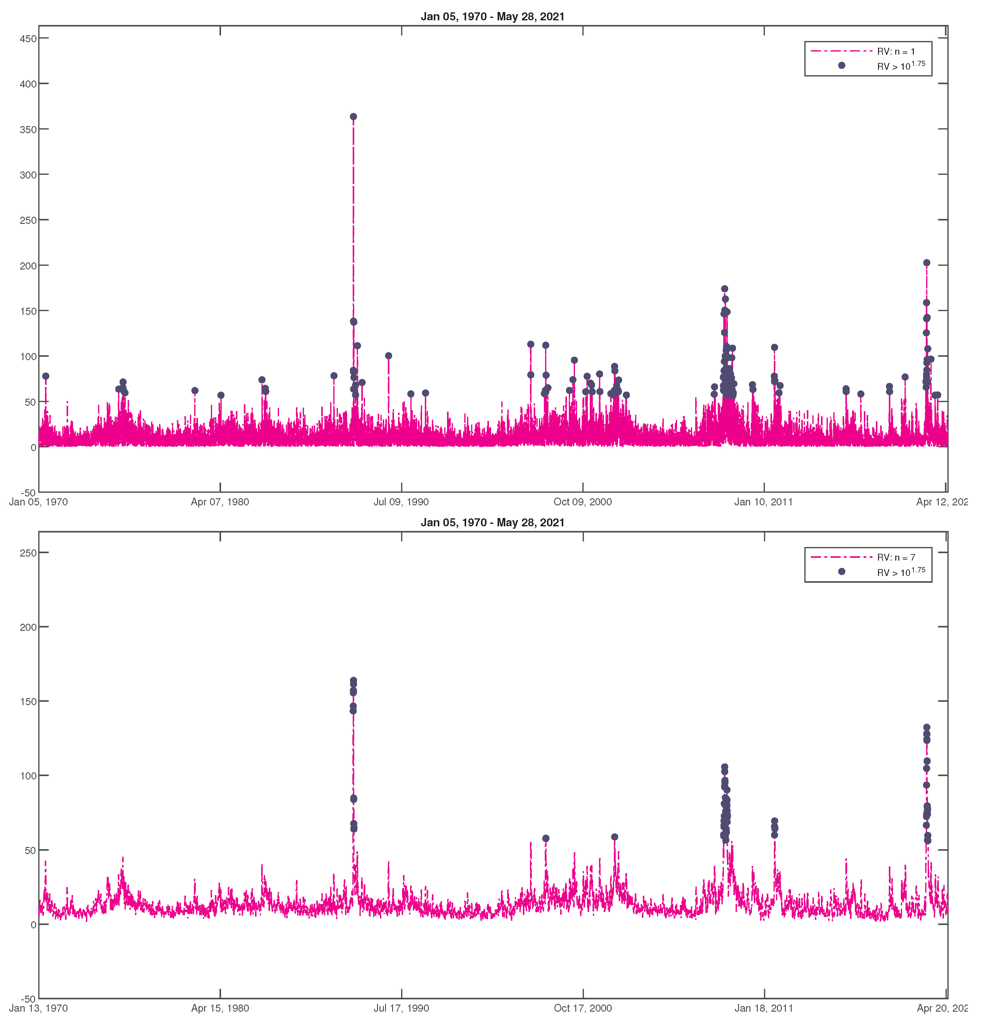
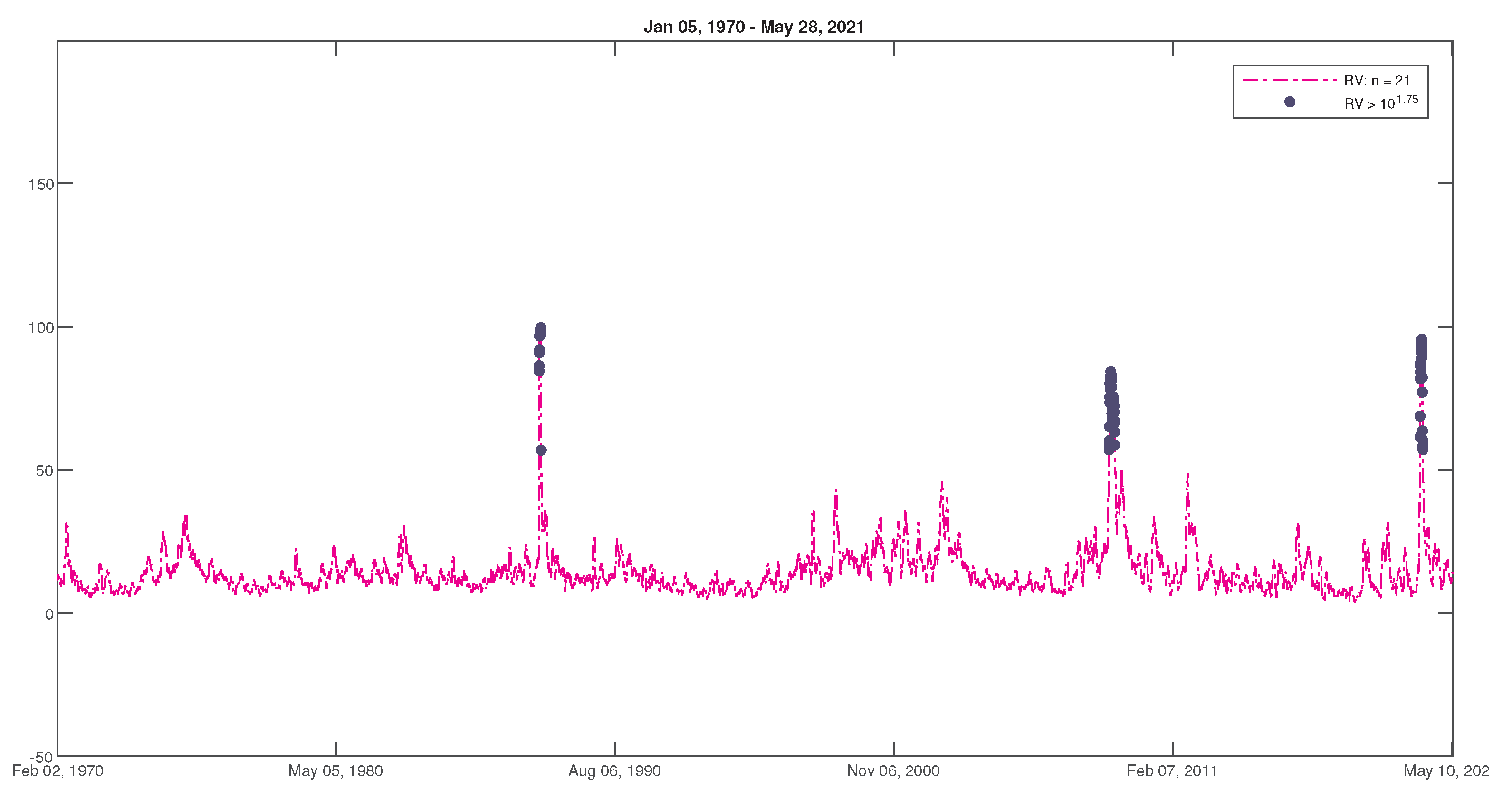
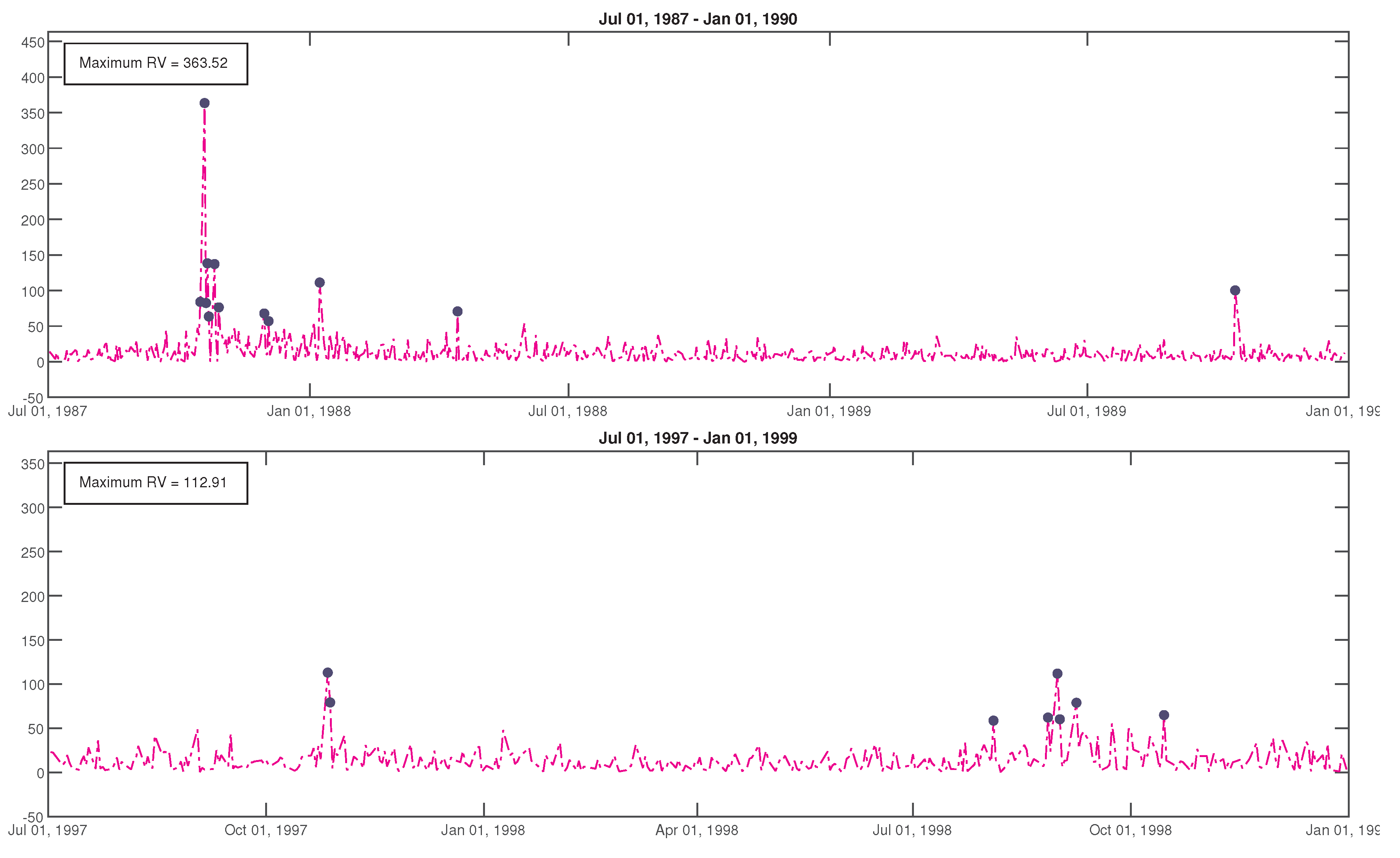
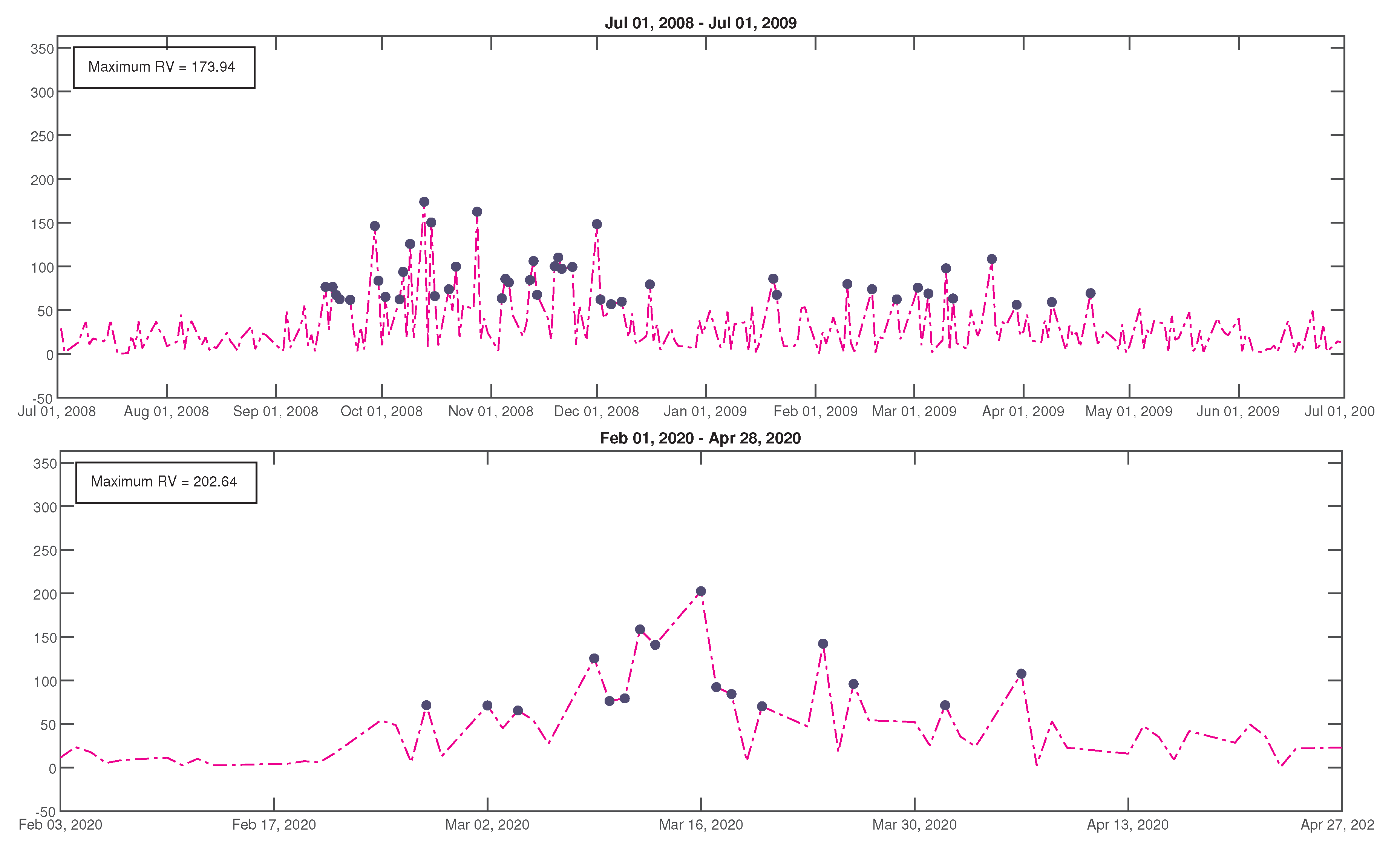
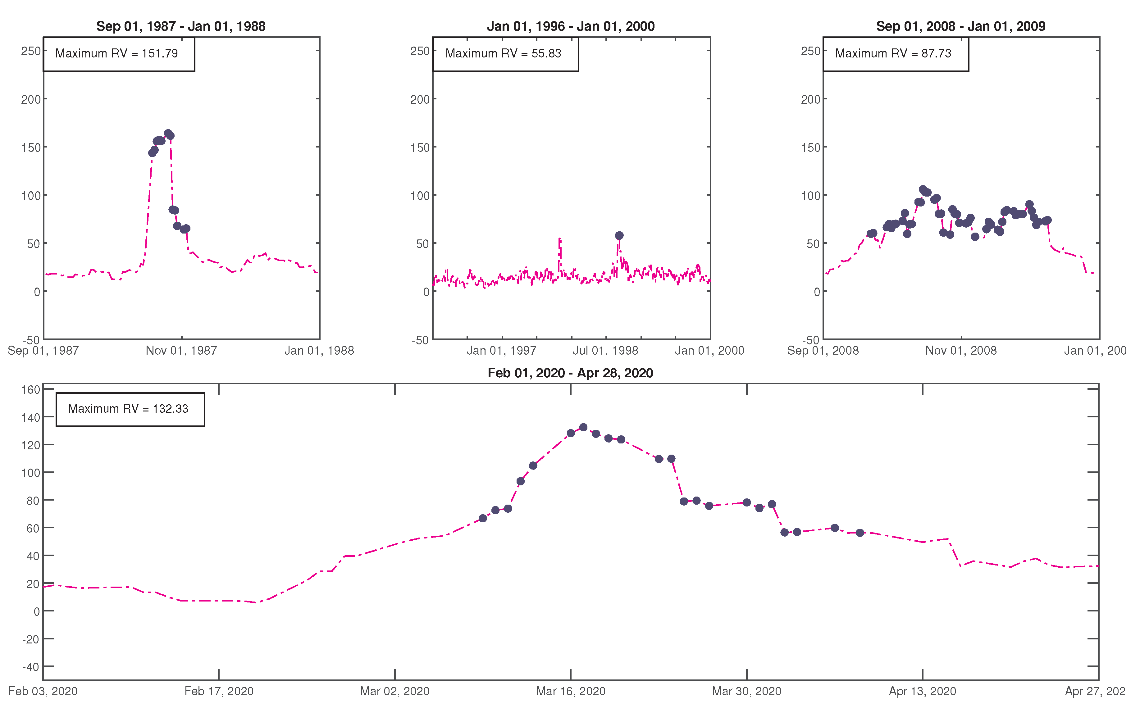
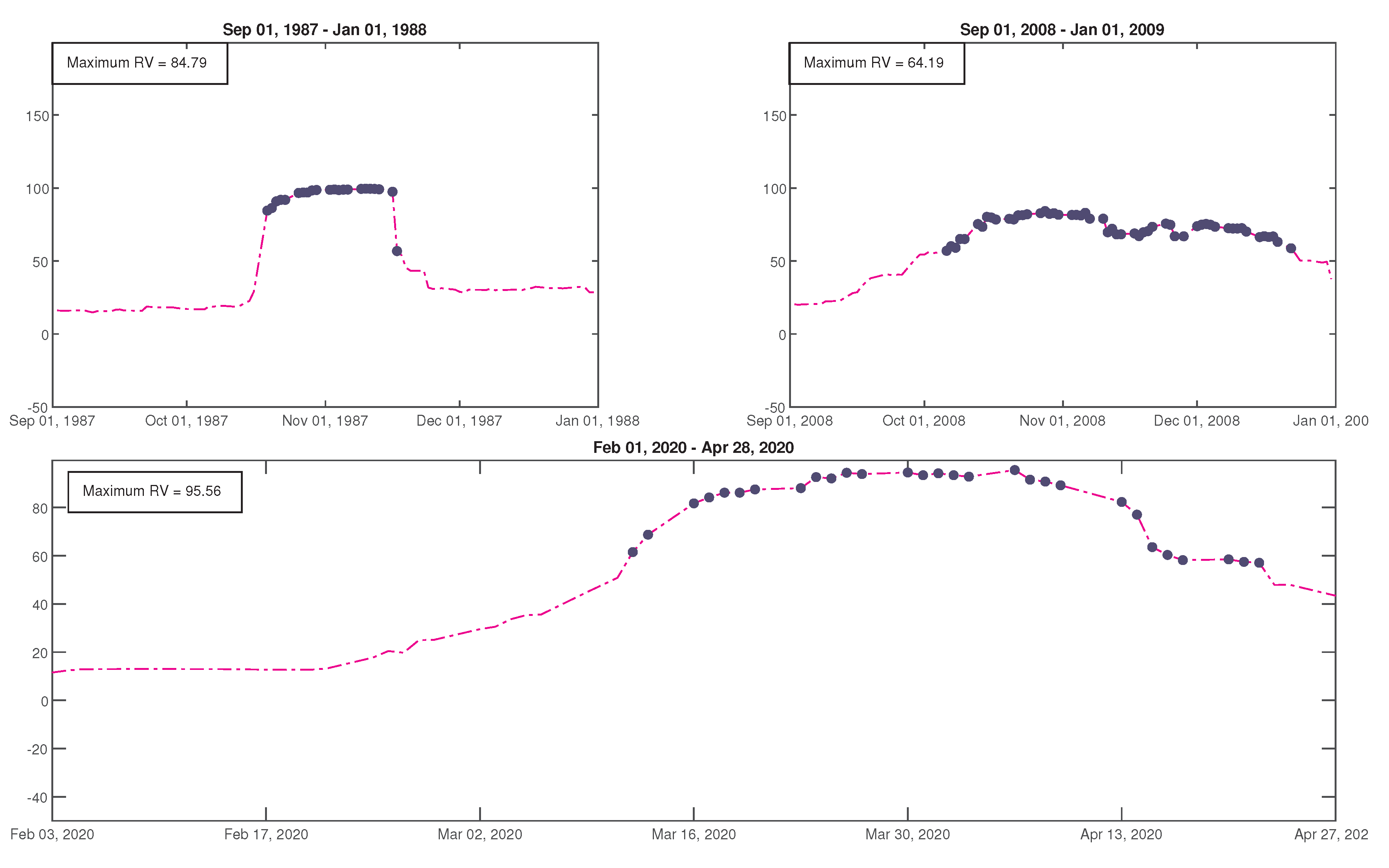
2. Time Series of Realized Volatility
3. Generalized Beta Distribution Function
4. Fitting Distribution of Realized Volatility
4.1. Methodology
4.2. Results
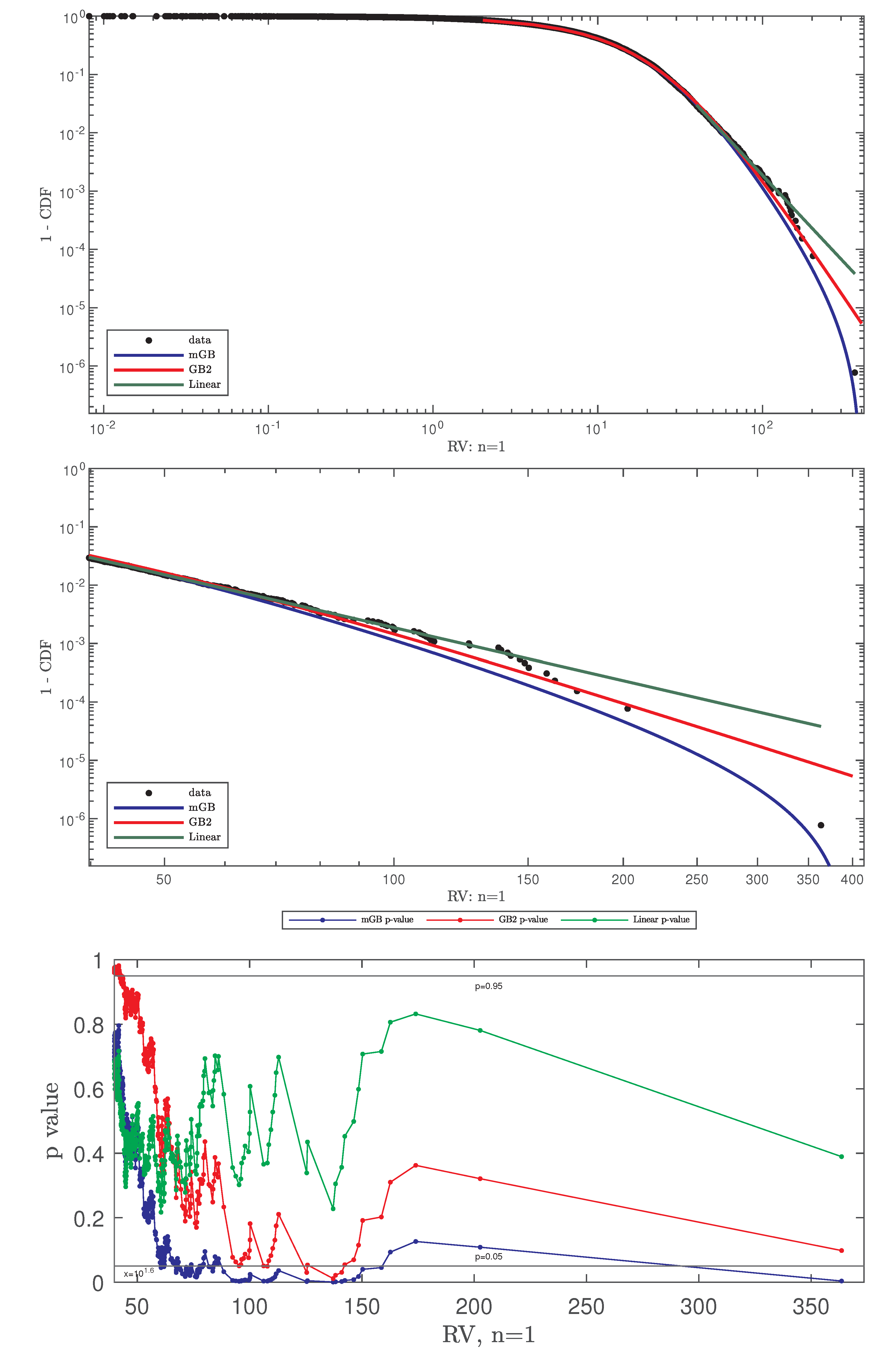
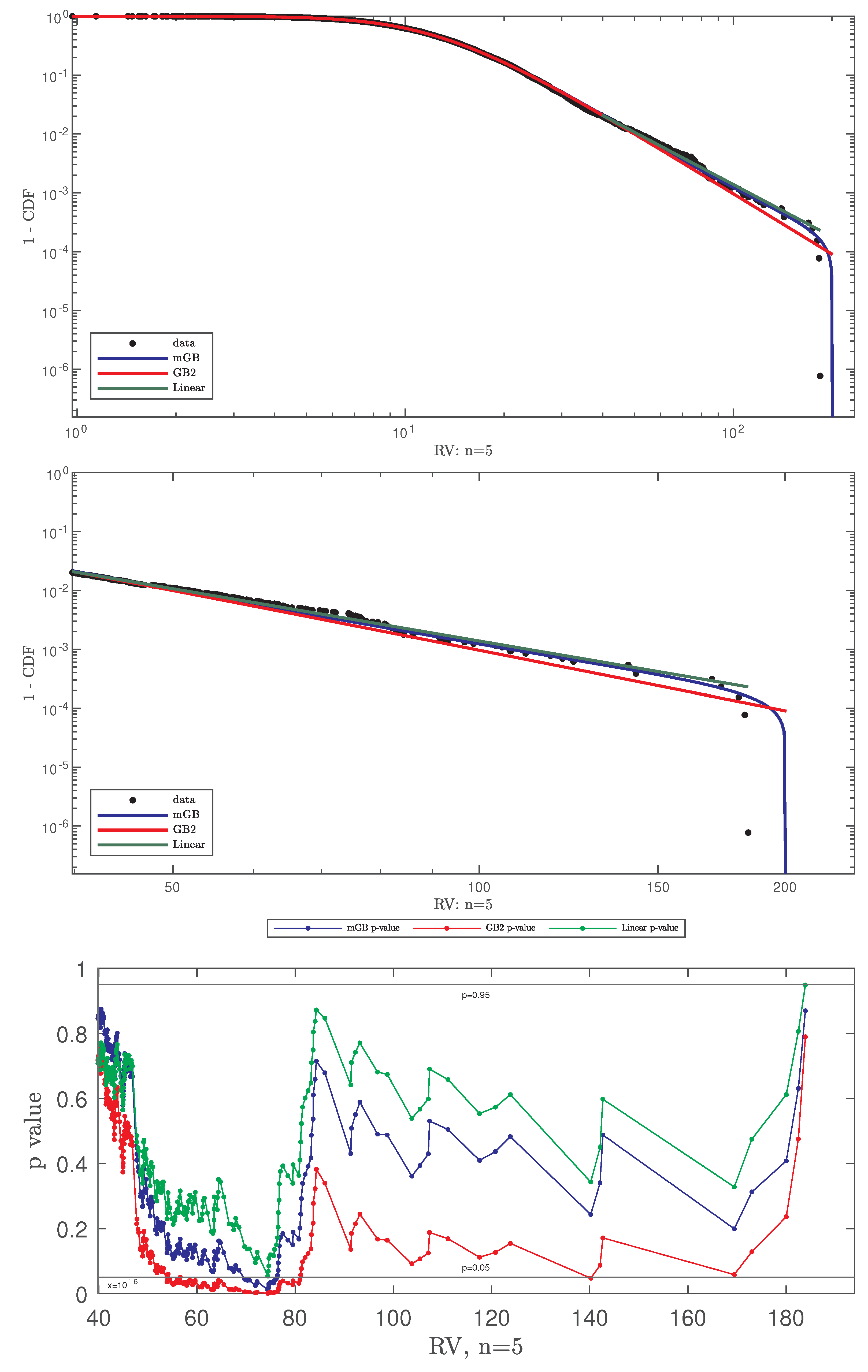
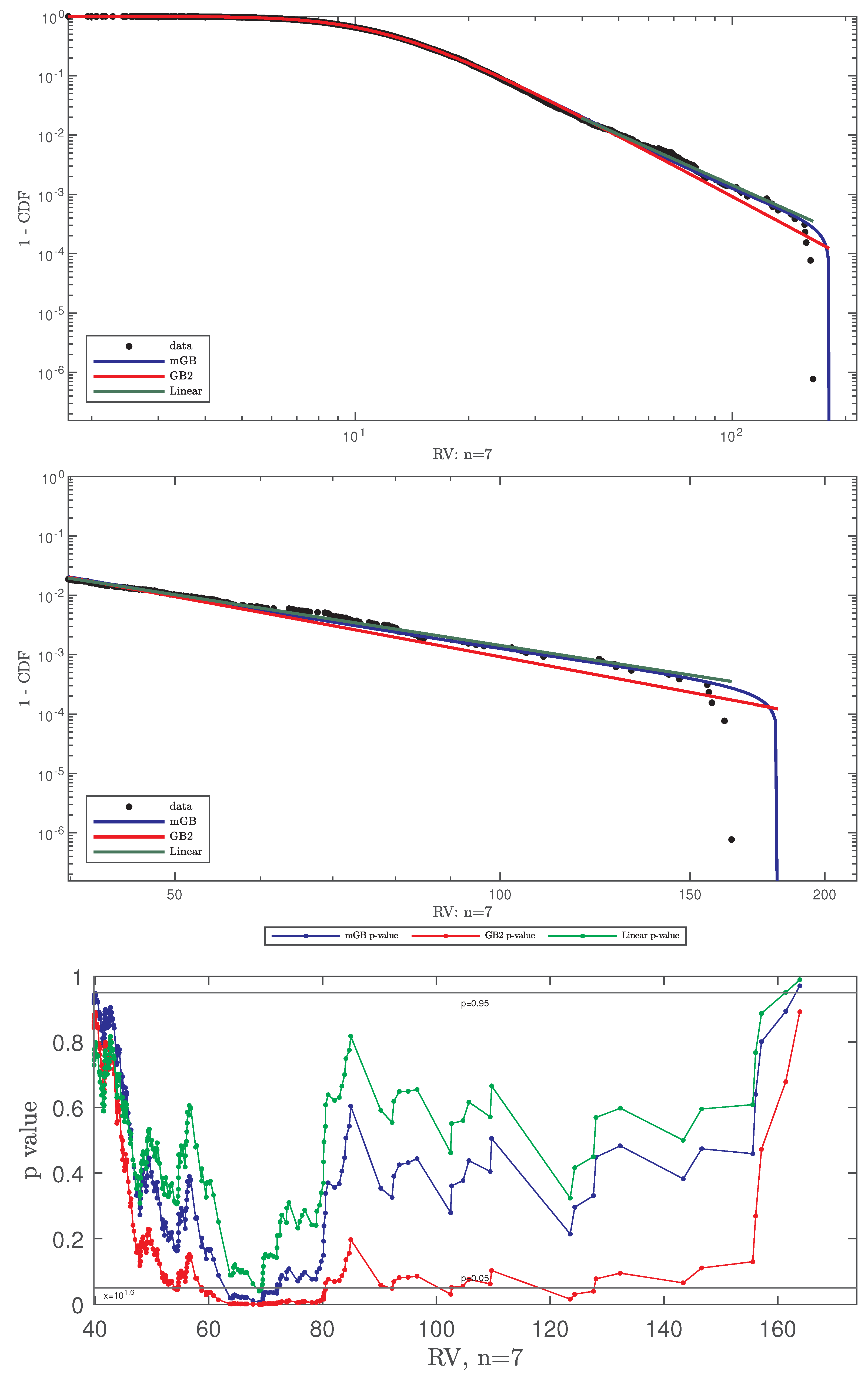
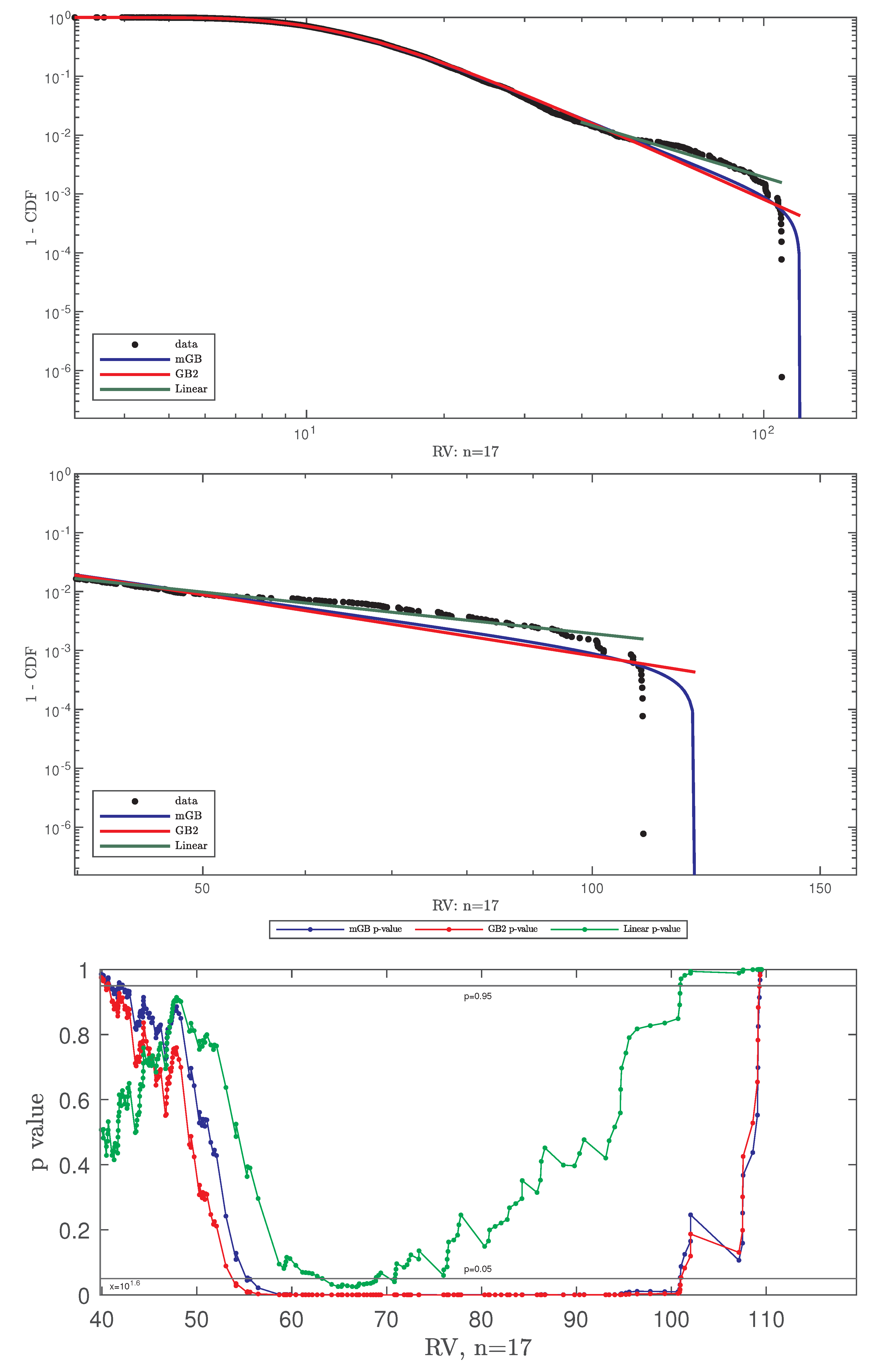
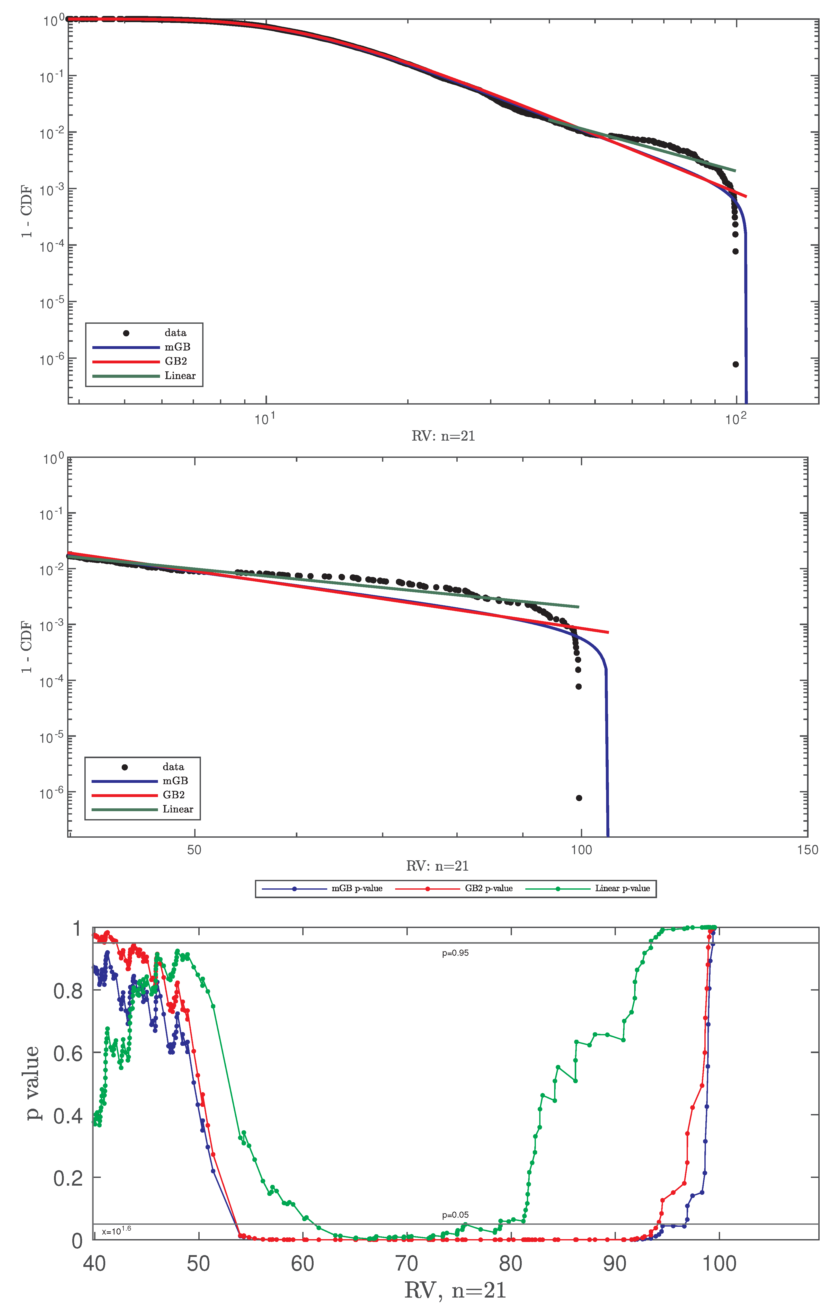
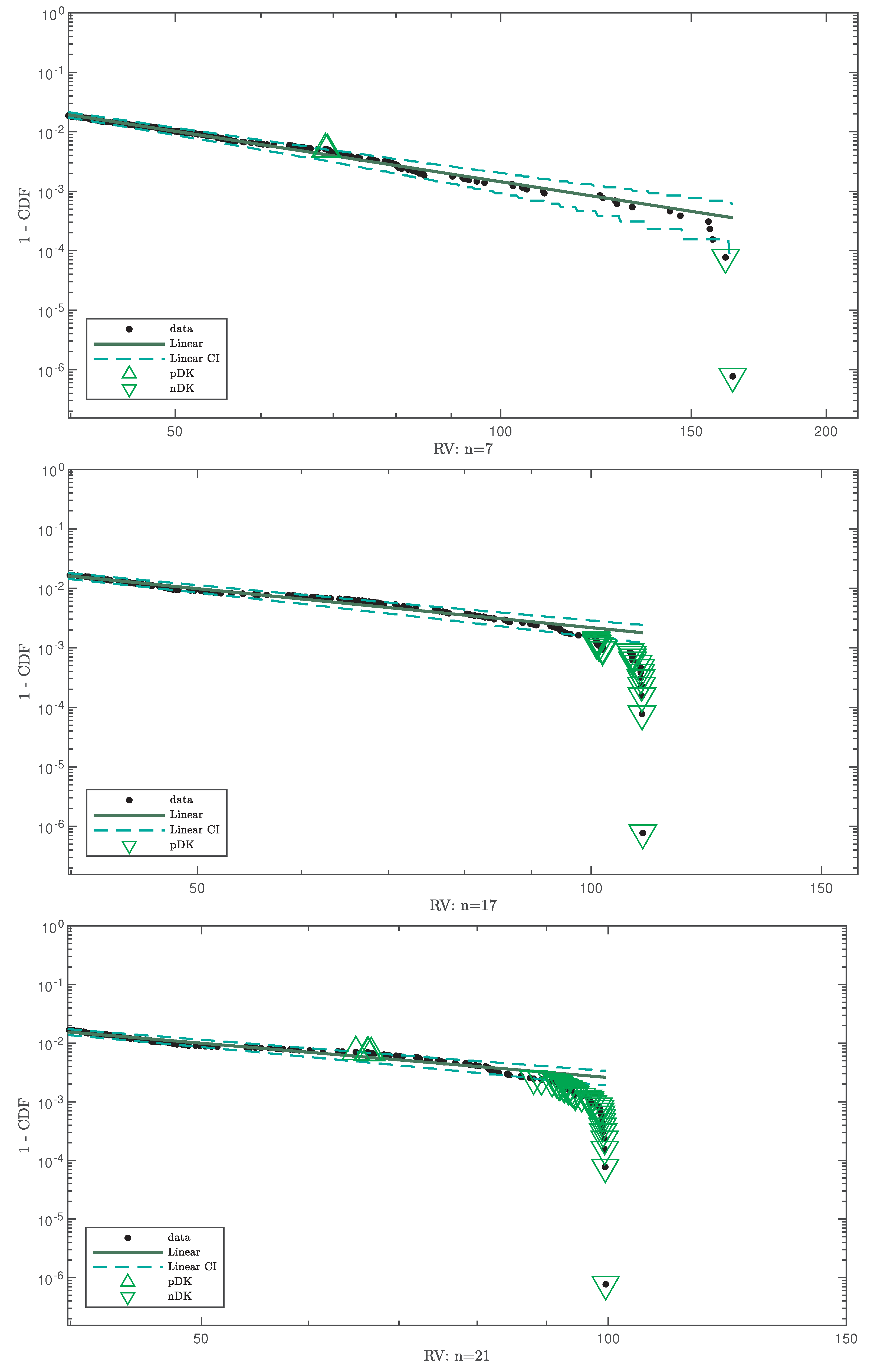
- Full data CDF fit with mGB and GB2 and LF of the tails;
- Same as above shown for ;
- p-values of all three fits for , with indicating DK and nDK;
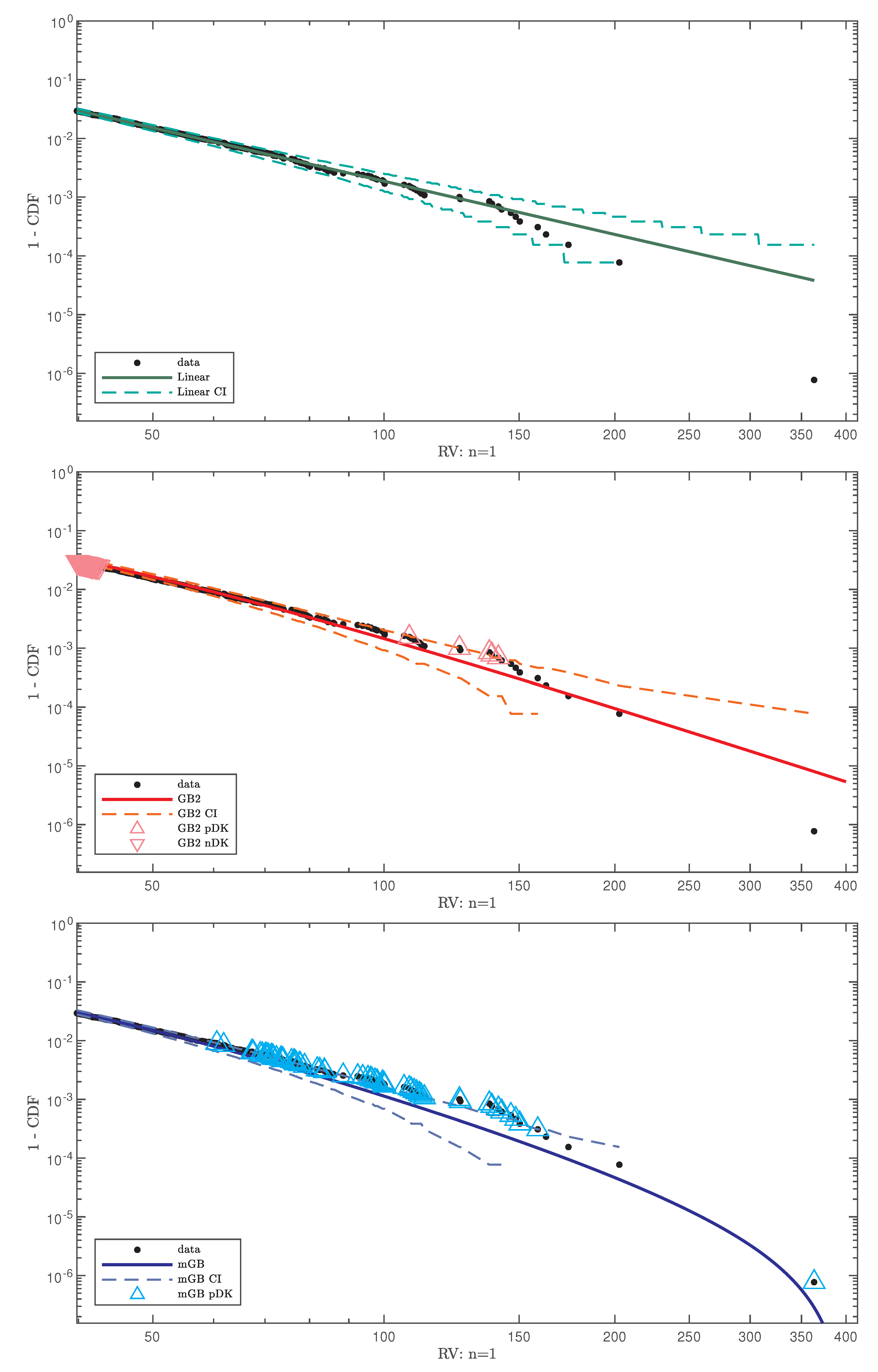
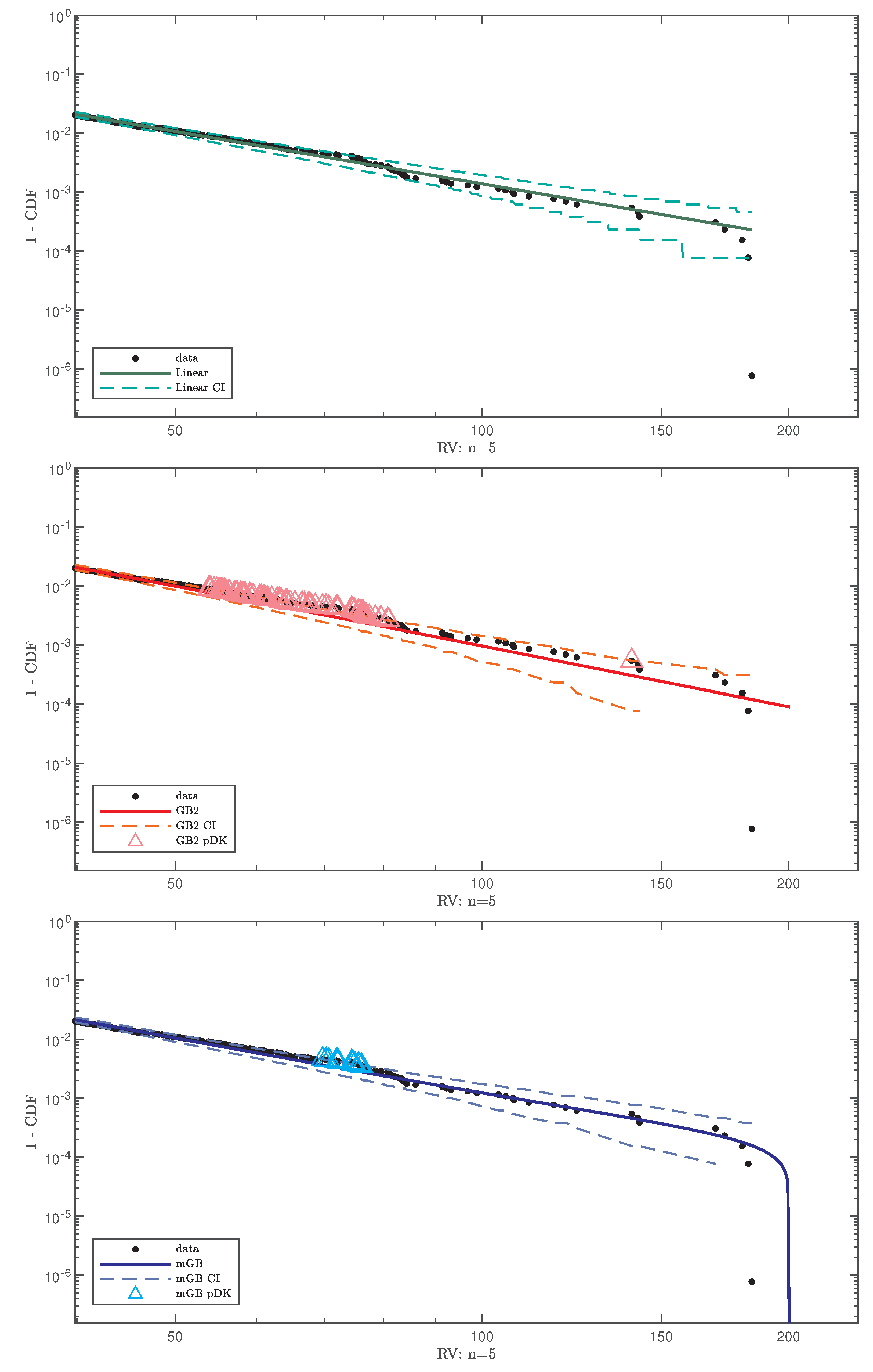
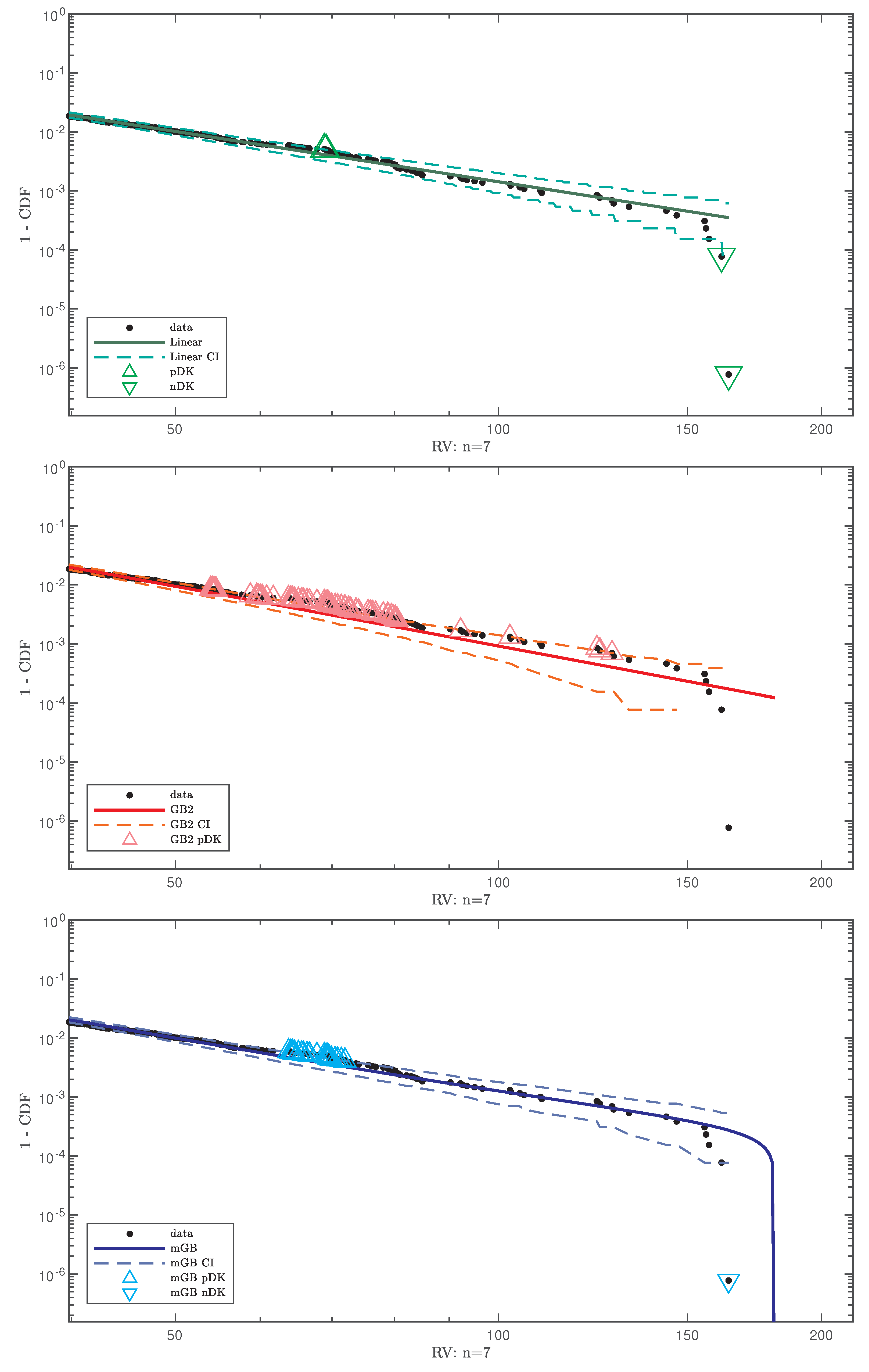
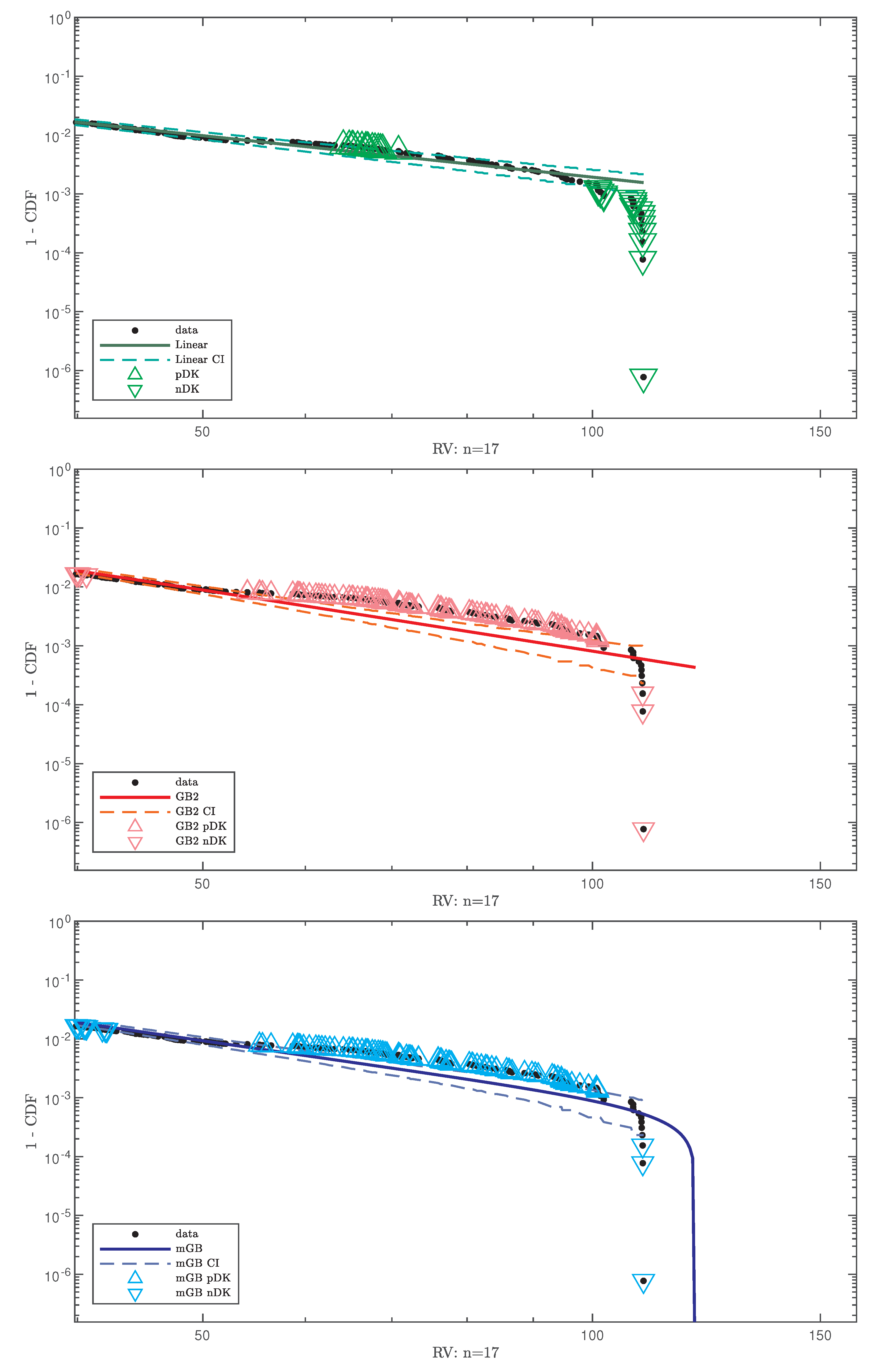
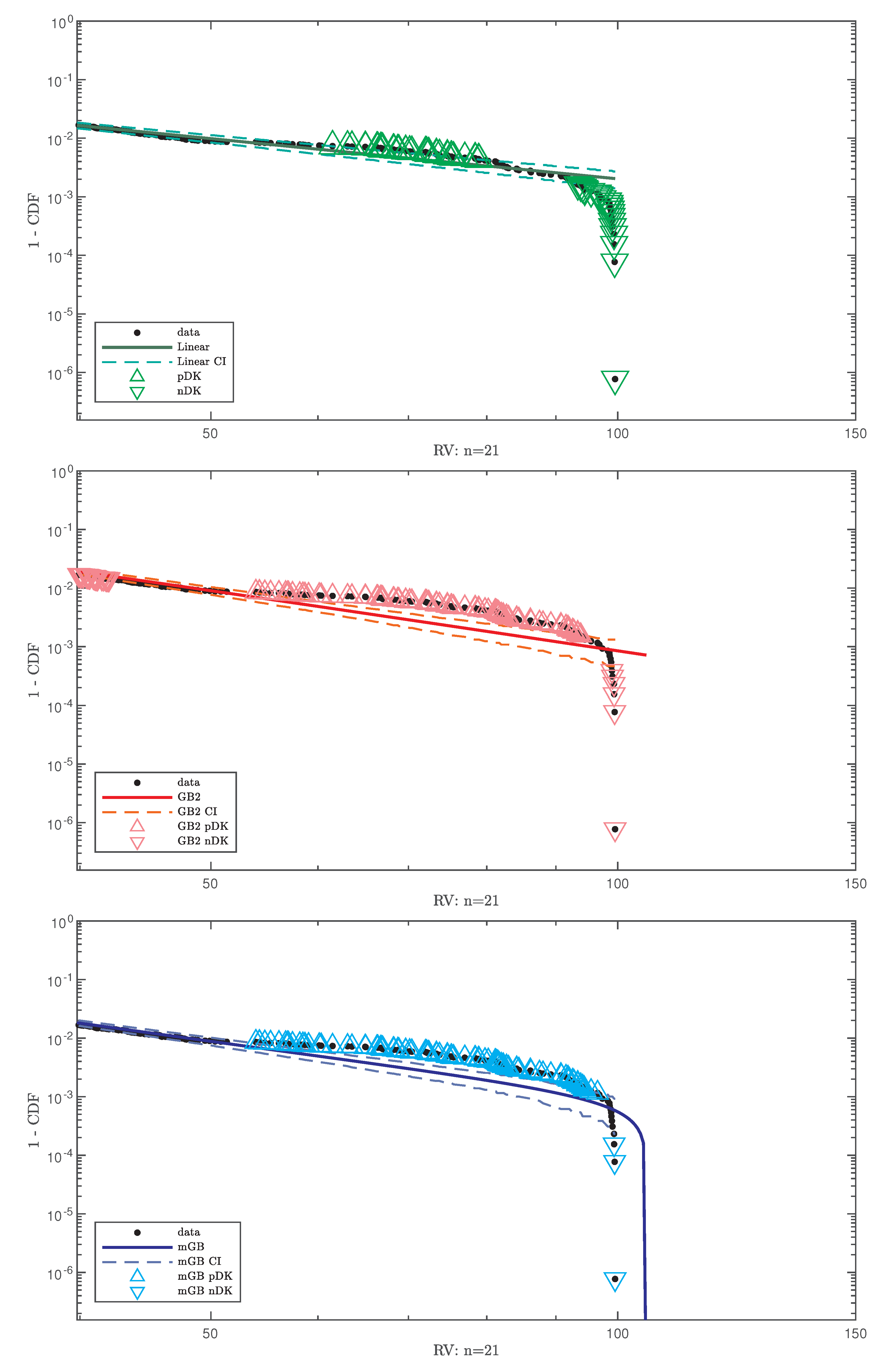
- LF with its CI;
- GB2 fit with its CI;
- mGB fit with its CI.
5. Discussion
6. Conclusions
Author Contributions
Funding
Data Availability Statement
Acknowledgments
Conflicts of Interest
References
- Clauset, A.; Shalizi, C.R.; Newman, M.E. Power-Law Distributions in Empirical Data. SIAM Rev. 2009, 51, 661–703. [Google Scholar] [CrossRef]
- Gabaix, X. Power laws in economics and finance. Annu. Rev. Econ. 2009, 1, 255–294. [Google Scholar] [CrossRef]
- Saichev, A.; Malevergne, Y.; Sornette, D. Theory of Zipf’s Law and Beyond; Lecture Notes in Economics and Mathematical Systems; Springer: Berlin/Heidelberg, Germany, 2009. [Google Scholar]
- Janczura, J.; Weron, R. Black swans or dragon-kings? A simple test for deviations from the power law. Eur. Phys. J. Spec. Top. 2012, 205, 79–93. [Google Scholar] [CrossRef]
- Pisarenko, V.F.; Sornette, D. Robust statistical tests of Dragon-Kings beyond power law distribution. Eur. Phys. J. Spec. Top. 2012, 205, 95–115. [Google Scholar] [CrossRef]
- Wheatley, S.; Sornette, D. Multiple Outlier Detection in Samples with Exponential Pareto Tails: Redeeming the Inward Approach Detecting Dragon Kings. arXiv 2015, arXiv:1507.08689. [Google Scholar] [CrossRef]
- Sornette, D. Dragon-Kings, Black Swans and the Prediction of Crises. Int. J. Terraspace Sci. Eng. 2009, 2, 1–18. [Google Scholar] [CrossRef]
- Sornette, D.; Ouillon, G. Dragon-kings: Mechanisms, statistical methods and empirical evidence. Eur. Phys. J. Spec. Top. 2012, 205, 1–26. [Google Scholar] [CrossRef]
- Golosovsky, M.; Solomon, S. Runaway events dominate the heavy tail of citation distributions. Eur. Phys. J. Spec. Top. 2012, 205, 303–311. [Google Scholar] [CrossRef]
- Medina, J.A. Extreme reaction times determine fluctuation scaling in human color vision. Phys. A 2016, 461, 125–132. [Google Scholar] [CrossRef]
- Johansen, A.; Sornette, D. Stock market crashes are outliers. Eur. Phys. J. B 1998, 1, 141–143. [Google Scholar] [CrossRef]
- Johansen, A.; Sornette, D. Large Stock Market Price Drawdowns Are Outliers. J. Risk 2001, 4, 69–110. [Google Scholar] [CrossRef]
- Sornette, D.; Johansen, A. Significance of log-periodic precursors to financial crashes. Quant. Financ. 2001, 1, 452–471. [Google Scholar] [CrossRef]
- Filimonov, V.; Sornette, D. Power law scaling and “Dragon-Kings” in distributions of intraday financial drawdowns. Chaos Solitons Fractals 2015, 74, 27–45. [Google Scholar] [CrossRef]
- CBOE VIX Index. Available online: https://www.cboe.com/tradable_products/vix/ (accessed on 1 January 2024).
- VIX Options and Futures Historical Data. Available online: http://www.cboe.com/products/vix-index-volatility/vix-options-and-futures/vix-index/vix-historical-data (accessed on 1 January 2024).
- Demeterfi, K.; Derman, E.; Kamal, M.; Zou, J. A guide to volatility and variance swaps. J. Deriv. 1999, 6, 9–32. [Google Scholar] [CrossRef]
- The CBOE Volatility Index—VIX. Previous Location of VIX White Paper, Appears to Have Been Since Removed. 2003. Available online: https://www.cboe.com/micro/vix/vixwhite.pdf (accessed on 1 January 2024).
- Chrstensen, B.J.; Prabhala, N.R. The Relation Between Implied and Realized Volaility. J. Financ. Econ. 1998, 50, 125–150. [Google Scholar] [CrossRef]
- Vodenska, I.; Chambers, W.J. Understanding the Relationship between VIX and the S&P 500 Index Volatility. In Proceedings of the 26th Australasian Finance and Banking Conference, Sydney, Australia, 17–19 December 2013. [Google Scholar]
- Kownatzki, C. How good is the VIX as a predictor of market risk? J. Account. Financ. 2016, 16, 39–60. [Google Scholar]
- Russon, M.D.; Vakil, A.F. On the non-linear relationship between VIX and realized SP500 volatility. Invest. Manag. Financ. Innov. 2017, 14, 200–206. [Google Scholar] [CrossRef]
- Dashti Moghaddam, M.; Liu, Z.; Serota, R.A. Distributions of Historic Market Data—Implied and Realized Volatility. Appl. Econ. Financ. 2019, 6, 104–130. [Google Scholar] [CrossRef]
- Dashti Moghaddam, M.; Liu, J.; Serota, R.A. Implied and Realized Volatility: A Study of Distributions and Distribution of Difference. Int. J. Financ. Econ. 2021, 26, 2581–2594. [Google Scholar] [CrossRef]
- Liu, J.; Serota, R.A. Rethinking Generalized Beta family of distributions. Eur. Phys. J. B 2023, 96, 24. [Google Scholar] [CrossRef]
- McDonald, J.B.; Xu, Y.J. A generlazition of the beta distribution with applications. J. Econom. 1996, 66, 133–152. [Google Scholar] [CrossRef]
- Risken, H. The Fokker-Planck Equation; Springer: Berlin/Heidelberg, Germany, 1996. [Google Scholar]
- Hertzler, G. “Classical” Probability Distributions for Stochastic Dynamic Models. In Proceedings of the 47th Annual Conference of the Australian Agricultural and Resource Economics Society, Fremantle, Australia, 12–14 February 2003. [Google Scholar]
- Jacobs, K. Stochastic Processes for Physicists; Cambridge University Press: Cambridge, UK, 2010. [Google Scholar]
- Dashti Moghaddam, M.; Serota, R.A. Combined Mutiplicative-Heston Model for Stochastic Volatility. Phys. A Stat. Mech. Its Appl. 2021, 561, 125263. [Google Scholar] [CrossRef]
- NIST Digital Library of Mathematical Functions. Available online: https://dlmf.nist.gov (accessed on 6 February 2024).
- Massey, F.J. The Kolmogorov-Smirnov Test for Goodness of Fit. J. Am. Stat. Assoc. 1985, 80, 954–958. [Google Scholar] [CrossRef]
- Liu, Z.; Dashti Moghaddam, M.; Serota, R.A. Distributions of Historic Market Data—Stock Returns. Eur. Phys. J. B 2019, 92, 60. [Google Scholar] [CrossRef]
- Dashti Moghaddam, M.; Liu, Z.; Serota, R.A. Distributions of historic market data: Relaxation and correlations. Eur. Phys. J. B 2021, 94, 83. [Google Scholar] [CrossRef]
- Liu, J.; Farahani, H.; Serota, R.A. Exploring distributions of housing prices and housing prices index. arXiv 2023, arXiv:2312.14325. [Google Scholar]


| n | Parameters of | Parameters of |
|---|---|---|
| 1 | ||
| 5 | ||
| 7 | ||
| 17 | ||
| 21 |
| n | SE of Parameters of | SE of Parameters of |
|---|---|---|
| 1 | ||
| 5 | ||
| 7 | ||
| 17 | ||
| 21 |
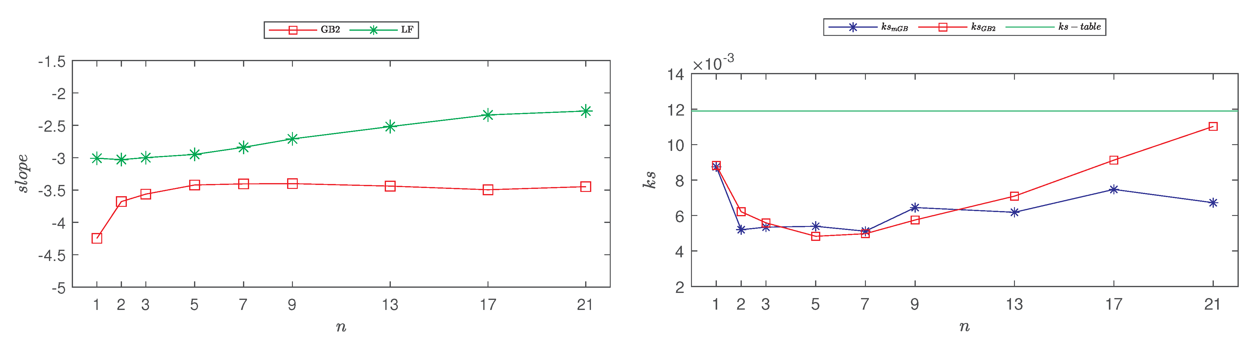
| n | LF | |
|---|---|---|
| 1 | −4.25 | −3.01 |
| 5 | −3.42 | −2.95 |
| 7 | −3.41 | −2.84 |
| 17 | −3.50 | −2.34 |
| 21 | −3.45 | −2.28 |
Disclaimer/Publisher’s Note: The statements, opinions and data contained in all publications are solely those of the individual author(s) and contributor(s) and not of MDPI and/or the editor(s). MDPI and/or the editor(s) disclaim responsibility for any injury to people or property resulting from any ideas, methods, instructions or products referred to in the content. |
© 2024 by the authors. Licensee MDPI, Basel, Switzerland. This article is an open access article distributed under the terms and conditions of the Creative Commons Attribution (CC BY) license (https://creativecommons.org/licenses/by/4.0/).
Share and Cite
Liu, J.; Dashti Moghaddam, M.; Serota, R.A. Are There Dragon Kings in the Stock Market? Foundations 2024, 4, 91-113. https://doi.org/10.3390/foundations4010008
Liu J, Dashti Moghaddam M, Serota RA. Are There Dragon Kings in the Stock Market? Foundations. 2024; 4(1):91-113. https://doi.org/10.3390/foundations4010008
Chicago/Turabian StyleLiu, Jiong, Mohammadamin Dashti Moghaddam, and Rostislav A. Serota. 2024. "Are There Dragon Kings in the Stock Market?" Foundations 4, no. 1: 91-113. https://doi.org/10.3390/foundations4010008