Comparison between Two Competing Newton-Type High Convergence Order Schemes for Equations on Banach Spaces

Abstract

We carried out a local comparison between two ninth convergence order schemes for solving nonlinear equations, relying on first-order Fréchet derivatives. Earlier investigations require the existence as well as the boundedness of derivatives of a high order to prove the convergence of these schemes. However, these derivatives are not in the schemes. These assumptions restrict the applicability of the schemes, which may converge. Numerical results along with a boundary value problem are given to examine the theoretical results. Both schemes are symmetrical not only in the theoretical results (formation and convergence order), but the numerical and dynamical results are also similar. We calculated the convergence radii of the nonlinear schemes. Moreover, we obtained the extraneous fixed points for the proposed schemes, which are repulsive and are not part of the solution space. Lastly, the theoretical and numerical results are supported by the dynamic results, where we plotted basins of attraction for a selected test function.

1. Introduction

Let $F:\mathrm{\Omega }\subset E_1\to E_2$ be an operator, where $E_1$ and $E_2$ are Banach spaces and $\mathrm{\Omega }\ne \varphi$ is an open convex subset of $E_1$. F is a Fréchet differentiable operator at each point of $\mathrm{\Omega }$. We use this scheme to find a solution $x^{*}$ of the nonlinear operator equation in the form

$$F\left(x\right)=0.$$

(1)

Newton’s scheme is most commonly used for solving such equations. However, it is only of order two under some conditions ([1,2,3]). It is defined as follows

$$x_{n+1}=x_n-F^{\prime }{\left(x_n\right)}^{-1}F\left(x_n\right),n=0,1,2,\cdots .$$

(2)

There are several papers on the variation or modification of Newton’s scheme in real ([1,4]) and in Banach space ([5,6]) to achieve a higher order.

A plethora of iterative scheme of convergence orders three or higher [7,8,9,10,11,12,13,14] have been developed in the literature provided that $E_1=E_2=R^J$. Third convergence order schemes, each involving two linear mapping inversions, are given by Cordero and Torregrosa [15], Homeier [9], Grau- Sanchez et al. [16] and Noor and Waseem [17].

Cordero et al. [18] developed a fourth-order converging scheme involving the computation of two operators, two derivatives (first) and one linear mapping inversion. Sharma and Gupta provided in [19] a fifth convergence order scheme requiring the evaluation of two operators, two derivative (first) and two linear operator inversions. Other such schemes can be found in [20] and the references therein. The convergence orders can be extended further if multistep schemes are introduced involving more than two or three steps. Let us revisit two such schemes as follows:

Let k be a natural number; $H_1$ and $H_2$ denote the iteration function of order q. Define the k step schemes for each $n=0,1,2,\cdots ,$

$$\left\{\begin{array}{c}{x}_0\in \mathrm{\Omega },\hfill \\ y_n=x_n-F^{\prime }{\left(x_n\right)}^{-1}F\left(x_n\right),\hfill \\ z_n=H_1(x_n,y_n),\hfill \\ z_n^{\left(1\right)}=z_n-{\psi }_1(x_n,y_n)F\left(z_n\right),\hfill \\ ..........\hfill \\ z_n^{(k-1)}=z_n^{(k-2)}-{\psi }_1(x_n,y_n)F\left(z_n^{(k-2)}\right),\hfill \\ x_{n+1}=z_n^{\left(k\right)}=z_n^{(k-1)}-{\psi }_1(x_n,y_n)F\left(z_n^{(k-1)}\right),\hfill \end{array}\right.$$

(3)

and

$$\left\{\begin{array}{c}{x}_0\in \mathrm{\Omega },\hfill \\ y_n=x_n-F^{\prime }{\left(x_n\right)}^{-1}F\left(x_n\right),\hfill \\ z_n=H_2(x_n,y_n),\hfill \\ z_n^{\left(1\right)}=z_n-{\psi }_2(x_n,y_n)F\left(z_n\right),\hfill \\ ..........\hfill \\ z_n^{(k-1)}=z_n^{(k-2)}-{\psi }_2(x_n,y_n)F{\left(z_n\right)}^{(k-2)},\hfill \\ x_{n+1}=z_n^{\left(k\right)}=z_n^{(k-1)}-{\psi }_2(x_n,y_n)F{\left(z_n\right)}^{(k-1)},\hfill \end{array}\right.$$

(4)

where we define $A_n=3F^{\prime }\left(y_n\right)-F^{\prime }\left(x_n\right)$, $B_n=F^{\prime }{\left(y_n\right)}^{-1}{F}^{\prime }\left(x_n\right)F^{\prime }{\left(y_n\right)}^{-1}+F^{\prime }{\left(x_n\right)}^{-1}$, ${\psi }_1(x_n,y_n)=\frac{1}{3}(4A_n^{-1}+F^{\prime }{\left(x_n\right)}^{-1})$ and ${\psi }_2(x_n,y_n)=\frac{1}{2}{B}_n$.

Notice that both the schemes require k function evaluations and two inverses per complete step. The convergence order $q+3k$ is established by Xiao and Yin in [21,22], respectively. However, there exist limitations restricting the utilizations of the aforementioned schemes. Below is a list.

$\left[l_1\right]$—The boundedness and existence of at least $F^{\prime },F^{\left(2\right)},F^{\left(3\right)},F^{\left(4\right)}$ and even higher orders is assumed although only $F^{\prime }$ is on these schemes. There even exist equations on the real line, such as the results in the previous references, which cannot assure the convergence of the schemes to a solution $x^{*}\in \mathrm{\Omega }$ of the equation $F\left(x\right)=0.$ Let $\mathrm{\Omega }=[-0.45,1.45]$.

Define the function $F:\mathrm{\Omega }\to \Re$ as

$$F\left(t\right)=\left\{\begin{array}{c}-t^4+t^5+2t^{3}lnt,fort\ne 0,\hfill \\ 0,fort=0\hfill \end{array}\right.$$

The definition of the function F gives that $F^{\prime \prime \prime }\left(t\right)=22-24t+60t^2+12lnt$. The function $F^{\prime \prime \prime }\left(t\right)$ is not continuous at $t=0$ and $t^{*}=1\in \mathrm{\Omega }$ solves the equation $F\left(t\right)=0$. Thus, all the results requiring the existence of at least the third derivative of F cannot assure the convergence of the afforementioned scheme to $t^{*}$, although they may converge.

$\left[l_2\right]$—A priori estimates of $\mid \mid (x_n-x_{*})\mid \mid$ are not provided. Thus, it is not known in advance the number of iterations to be performed to satisfy a certain predecided error tolerance.

$\left[l_3\right]$—There is no information about if there are solutions other than $x_{*}\in \mathrm{\Omega }.$

$\left[l_4\right]$—The results are restricted in ${\Re }^j$.

Notice, however, that the schemes (1) and (2) are extended in the setting of Banach space. Limitations $\left(l_1\right)$–$\left(l_4\right)$ constitute the motivation for writing this article. Moreover, the novelty of this article is that the items $\left(l_1\right)$–$\left(l_4\right)$ are addressed positively as follows:

${\left[l_1\right]}^{\prime }$—The convergence is established using only $F^{\prime }$, which is in these schemes, and the idea of generalized continuity [5,18,20].

${\left[l_2\right]}^{\prime }$—The number of iterations to reach a predecided error tolerance is calculated.

${\left[l_3\right]}^{\prime }$—The isolation of $x_{*}$ is addressed.

${\left[l_4\right]}^{\prime }$ —The results are valid in Banach space.

The techniques to achieve the aforementioned objectives are demonstrated for some specializations of schemes (1) and (2). However, the technique can be analogously used on the rest of the schemes.

Let $k=2$;

$H_1(x_n,y_n)=x_n-\frac{2}{3}(A_n^{-1}+F{\left(x_n\right)}^{-1})F\left(x_n\right)$; and

$H_2(x_n,y_n)=x_n-\frac{1}{2}(F^{\prime }{\left(y_n\right)}^{-1}+F^{\prime }{\left(x_n\right)}^{-1})F\left(x_n\right).$

These iteration functions are of convergence order three. Therefore, (1) and (2) specialize to schemes of convergence order $3+3\times 2=9$, since $q=3$ and $k=2$. In particular, these specializations are of schemes (1) and (2), respectively.

The convergence order can be found using the following formula

$$\mu \left(COC\right)=\frac{ln\left(\mid \mid (x_{n+1}-x_{*})\mid \mid /\mid \mid (x_n-x_{*})\mid \mid \right)}{ln\left(\mid \mid (x_n-x_{*})\mid \mid /\mid \mid (x_{n-1}-x_{*})\mid \mid \right)},$$

(5)

or

$${\mu }_1\left(ACOC\right)=\frac{ln\left(\mid \mid (x_{n+1}-x_n)\mid \mid /\mid \mid (x_n-x_{n-1})\mid \mid \right)}{ln\left(\mid \mid (x_n-x_{n-1})\mid \mid /\mid \mid (x_{n-1}-x_{n-2})\mid \mid \right)}.$$

(6)

These computations do not require the $F^{\prime \prime \prime }$ or $x_{*}$ (in the case of Formula (6)).

We study the ball convergence comparison of the two ninth-order iterative schemes

$$\left\{\begin{array}{c}{x}_0\in \mathrm{\Omega }\hfill \\ y_n=x_n-F^{\prime }{\left(x_n\right)}^{-1}F\left(x_n\right),\hfill \\ z_n=x_n-2/3(A_n^{-1}+F^{\prime }{\left(x_n\right)}^{-1})F\left(x_n\right),\hfill \\ w_n=z_n-1/3(4A_n^{-1}+F^{\prime }{\left(x_n\right)}^{-1})F\left(z_n\right),\hfill \\ x_{n+1}=w_n-1/3(4A_n^{-1}+F^{\prime }{\left(x_n\right)}^{-1})F\left(w_n\right),\hfill \end{array}\right.$$

(7)

and

$$\left\{\begin{array}{c}{x}_0\in \mathrm{\Omega }\hfill \\ y_n=x_n-F^{\prime }{\left(x_n\right)}^{-1}F\left(x_n\right),\hfill \\ z_n=x_n-\frac{1}{2}(F^{\prime }{\left(y_n\right)}^{-1}+F^{\prime }{\left(x_n\right)}^{-1})F\left(x_n\right),\hfill \\ w_n=z_n-\frac{1}{2}{B}_{n}F\left(z_n\right),\hfill \\ x_{n+1}=w_n-\frac{1}{2}{B}_{n}F\left(w_n\right),\hfill \end{array}\right.$$

(8)

where $F^{\prime }\left(x\right)$ is the Fréchet derivative of operator F at the point $x\in \mathrm{\Omega }$.

Numerical results consist of the comparative study of the proposed schemes along with Newton’s scheme by using the some test functions for nonlinear equations, systems of equations and a boundary value problem. One important characteristic of this work is the comparability of the dynamics of the proposed schemes along with Newton’s scheme for the solution of nonlinear equations.

2. Convergence: Scheme 1

We describe the ball convergence of proposed schemes (3) and (4), which are based on some real functions and positive parameters. Let $T=[0,\infty )$.

Suppose:

(a) There exists a nondecreasing and continuous function (NDCF) $h_0$ from $T\to T$ such that equation

$$h_0\left(t\right)-1=0$$

(9)

has a minimal positive (MP) zero $R_0$. Set $T_0=[0,R_0)$. Consider (NDCF) function h from $T_0\to T$.

(b) Equation

$$v_1\left(t\right)-1=0$$

has an MP zero $r_1\in (0,R_0),$ where

$$v_1\left(t\right)=\frac{{\int }_0^{1}h\left((1-\tau )t\right)d\tau }{1-h_0\left(t\right)}.$$

(c) Equation

$$p\left(t\right)-1=0,$$

(10)

has an MP zero denoted by $r_p$, where

$$p\left(t\right)=\frac{1}{2}(3h_0\left(v_1\left(t\right)t\right)+h_0\left(t\right)).$$

Set $R_1=min\{R_0,R_p\}$ and $T_1=[0,R_1)$. Consider (NDCF) $h_1$ from $T_1\to T$ nondecreasing and continuous.

(d) Equation

$$v_2\left(t\right)-1=0,$$

(11)

has an MP zero denoted by $r_2\in (0,R_1)$, where

$$v_2\left(t\right)=v_1\left(t\right)+\frac{\left(h_0\left(t\right)+h_0\left(v_1\left(t\right)t\right)\right){\int }_0^1{h}_1\left(\tau t\right)d\tau }{2(1-h_0\left(t\right))(1-p\left(t\right))}.$$

(e) Equation

$$h_0\left(v_2\left(t\right)t\right)-1=0$$

(12)

has an MP zero denoted by $R_2$. Set $R_3=min\{R_1,R_2\}$ and $T_2=[0,R_3)$.

(f) Equation

$$v_3\left(t\right)-1=0$$

(13)

has an MP zero denoted by $r_3\in (0,R_3)$, where

$$\begin{array}{cc}\hfill v_3\left(t\right)& =[v_1\left(v_2\left(t\right)t\right)+\frac{\left(h_0\left(t\right)+h_0\left(v_2\left(t\right)t\right)\right){\int }_0^1{h}_1\left(\tau v_2\left(t\right)t\right)d\tau }{(1-h_0\left(t\right))(1-h_0\left(v_2\left(t\right)t\right))}\hfill \\ \hfill & +\frac{\left(h_0\left(t\right)+h_0\left(v_1\left(t\right)t\right)\right){\int }_0^1{h}_1\left(\tau v_2\left(t\right)t\right)d\tau }{(1-h_0\left(t\right))(1-p\left(t\right))}]v_2\left(t\right).\hfill \end{array}$$

(g) Equation

$$h_0\left(v_3\left(t\right)t\right)-1=0$$

(14)

has an MP zero denoted by $R_4$. Set $R_5=min\{R_3,R_4\}$ and $T_3=[0,R_5)$.

(h) Equation

$$v_4\left(t\right)-1=0$$

(15)

has a minimal positive zero denoted by $r_4\in (0,R_5)$, where

$$\begin{array}{cc}\hfill v_4\left(t\right)& =[v_1\left(v_3\left(t\right)t\right)+\frac{\left(h_0\left(t\right)+h_0\left(v_3\left(t\right)t\right)\right){\int }_0^1{h}_1\left(\tau v_3\left(t\right)t\right)d\tau }{(1-h_0\left(t\right))(1-h_0\left(v_3\left(t\right)t\right))}\hfill \\ \hfill & +\frac{\left(h_0\left(t\right)+h_0\left(v_1\left(t\right)t\right)\right){\int }_0^1{h}_1\left(\tau v_3\left(t\right)t\right)d\tau }{(1-h_0\left(t\right))(1-p\left(t\right))}]v_3\left(t\right).\hfill \end{array}$$

We shall show that parameter $\rho$, given by

$$r=min\left\{r_k\right\},k=1,2,3,4,$$

(16)

is a convergence radius for scheme (3). By this definition, it follows for all $t\in [0,r)$ that

$$0\le h_0\left(t\right)<1,$$

(17)

$$0\le h_0\left(v_2\left(t\right)t\right)<1,$$

(18)

$$0\le h_0\left(v_3\left(t\right)t\right)<1,$$

(19)

$$0\le p\left(t\right)<1$$

(20)

and

$$0\le v_k\left(t\right)<1,i=1,2,3,4.$$

(21)

Let $S(x_{*},r)$ and $\overline{S}(x_{*},r)$ denote the open and closed balls in $B_1$, respectively, of center $x_{*}$ and radius $r>0.$

Next, we list the hypotheses in hypothesis $\left(A\right)$ used in our convergence analysis. They relate to the functions as described previously.

Suppose:

$\left(a_1\right)F:\mathrm{\Omega }\to B_2$ is continuously differentiable and there exists a simple solution $x_{*}$ of equation $F\left(x\right)=0$.

$\left(a_2\right)$ For all $x\in \mathrm{\Omega }$,

$$||F^{\prime }{\left(x_{*}\right)}^{-1}(F^{\prime }\left(x\right)-F^{\prime }\left(x_{*}\right)||\le h_0||(x-x_{*}||).$$

Set ${\mathrm{\Omega }}_0=\mathrm{\Omega }\cap S(x_{*},{\rho }_0).$

$\left(a_3\right)$ For all $x,y\in {\mathrm{\Omega }}_0$,

$$||F^{\prime }{\left(x_{*}\right)}^{-1}(F^{\prime }\left(y\right)-F^{\prime }\left(x_{*}\right)||\le h\left(||y-x_{*}||\right).$$

$$||F^{\prime }{\left(x_{*}\right)}^{-1}{F}^{\prime }\left(x\right)||\le h_1\left(||x-x_{*}||\right).$$

$\left(a_4\right)$$\overline{S}(x_{*},\tilde{r})\subset \mathrm{\Omega }$, where $\tilde{r}>0$ is to be determined.

$\left(a_5\right)$ There exists $r_{*}\ge \tilde{r}$ such that

$${\int }_0^1{h}_0\left(\tau r_{*}\right)d\tau <1.$$

Set

$${\mathrm{\Omega }}_1=\mathrm{\Omega }\cap \overline{S}(x_{*},r_{*}).$$

Based on hypothesis $\left(A\right)$ and the developed notation, we show the local convergence result for scheme (3).

Theorem 1.

Under the hypotheses in $\left(A\right)$ for $\tilde{r}=r$, further suppose $x_0\in S(x_{*},r)-\left\{x_{*}\right\}$. Then, the sequence generated by scheme (3) starting at $x_0$ is well defined, remains in $S(x_{*},r)-\left\{x_{*}\right\}$ and converges at $x_{*}$. Moreover, the following estimates hold true

$$||y_n-x_{*}||\le v_1\left(||x_n-x_{*}||\right)||x_n-x_{*}||\le ||x_n-x_{*}||<r,$$

(22)

$$\mid \mid z_n-x_{*}\mid \mid \le v_2(\mid \mid x_n-x_{*}\mid \mid )\mid \mid x_n-x_{*}\mid \mid \le \mid \mid x_n-x_{*}\mid \mid ,$$

(23)

$$\mid \mid w_n-x_{*}\mid \mid \le v_3(\mid \mid x_n-x_{*}\mid \mid )\mid \mid x_n-x_{*}\mid \mid \le \mid \mid x_n-x_{*}\mid \mid ,$$

(24)

$$\mid \mid x_{n+1}-x_{*}\mid \mid \le v_4(\mid \mid x_n-x_{*}\mid \mid )\mid \mid x_n-x_{*}\mid \mid \le \mid \mid x_n-x_{*}\mid \mid ,$$

(25)

where functions $v_k$ are defined earlier and r is given by (16). Furthermore, $x_{*}$ is unique as a solution of equation $F\left(x\right)=0$ in the domain ${\mathrm{\Omega }}_1$, given in $\left(a_5\right)$.

Proof. 

We shall prove items (22)–(25) using Induction. Consider $x\in S(x_{*},r)-x_{*}$. Then, using $\left(a_1\right)$ and $\left(a_2\right)$, we have

$$||F^{\prime }{\left(x_{*}\right)}^{-1}(F^{\prime }\left(x\right)-F^{\prime }\left(x_{*}\right))||\le h_0||x-x_{*}||\le h_0\left(r\right)<1.$$

Using the Banach lemma on invertible operators [12] and the preceding inequality, $F^{\prime }{\left(x\right)}^{-1}$ exists so that

$$||F^{\prime }{\left(x\right)}^{-1}{F}^{\prime }\left(x_{*}\right)||\le \frac{1}{1-h_0(\mid \mid x-x_{*}\mid \mid )}.$$

(26)

In particular, if $x=x_0$, $F^{\prime }{\left(x_0\right)}^{-1}$ exists, since $x_0\in S(x_{*},r)$. Then, the iterate $y_0$ exists by the first substep of scheme (3). We can write

$$\begin{array}{cc}\hfill ||y_0-x_{*}||& =||x_0-x_{*}-F^{\prime }{\left(x_0\right)}^{-1}F\left(x_0\right)||\hfill \\ \hfill & \le ||F^{\prime }{\left(x_0\right)}^{-1}{F}^{\prime }\left(x_{*}\right)||\hfill \\ \hfill & \times ||{\int }_0^1{F}^{\prime }{\left(x_{*}\right)}^{-1}\left(F^{\prime }(x_{*}+\tau (x_0-x_{*}))-F^{\prime }\left(x_0\right)\right)(x_0-x_{*})d\tau ||\hfill \end{array}$$

So, by conditions $\left(a_1\right)$, $\left(a_3\right)$ and (16) and (26),

$$\begin{array}{ccc}\hfill ||y_0-x_{*}||& \le & \frac{{\int }_0^{1}h\left((1-\tau )\right)||x_0-x_{*}||d\tau ||x_0-x_{*}||}{1-h_0\left(||x_0-x_{*}||\right)}\hfill \\ \hfill & \le & v_1(\mid \mid x_0-x_{*}\mid \mid )\mid \mid x_0-x_{*}\mid \mid \hfill \\ \hfill & \le & \mid \mid x_0-x_{*}\mid \mid \hfill \\ & <& r.\hfill \end{array}$$

(27)

Hence, the iterate $y_0\in S(x_{*},r)$ and (22) is valid for n = 0. We should show $A_0$ is invertible, so $z_0,v_0$ and $x_1$ exist by scheme (3) for n = 0. Indeed, we have by $\left(a_2\right)$, (17), (26) and (27)

$$\begin{array}{ccc}\hfill & & ||{\left(2F^{\prime }\left(x_{*}\right)\right)}^{-1}(A_0-2F^{\prime }\left(x_{*}\right))||\hfill \\ \hfill & \le & ||{\left(2F^{\prime }\left(x_{*}\right)\right)}^{-1}(3(F^{\prime }\left(y_0\right)-F^{\prime }\left(x_{*}\right))+(F^{\prime }\left(x_{*}\right)-F^{\prime }\left(x_0\right))||\hfill \\ \hfill & \le & \frac{1}{2}{[3\mid \mid F^{\prime }\left(x_{*}\right))}^{-1}(F^{\prime }\left(y_0\right)-F^{\prime }\left(x_{*}\right))\mid \mid +\mid \mid F^{\prime }\left(x_{*}\right){)}^{-1}(F^{\prime }\left(x_0\right)-F^{\prime }\left(x_{*}\right))\mid \mid ]\hfill \\ \hfill & \le & \frac{1}{2}(h_0(\mid \mid x_0-x_{*}\mid \mid )+3h_0(\mid \mid y_0-x_{*}\mid \mid ))\hfill \\ \hfill & \le & \frac{1}{2}(h_0(\mid \mid x_0-x_{*}\mid \mid )+3h_0(v_1(\mid \mid x_0-x_{*}\mid \mid )\mid \mid x_0-x_{*}\mid \mid ))\hfill \\ \hfill & \le & p(\mid \mid x_0-x_{*}\mid \mid )\le p\left(r\right)<1.\hfill \end{array}$$

Thus, the linear operator $A_0$ is invertible and

$$||A_0^{-1}{F}^{\prime }\left(x_{*}\right)||\le \frac{1}{2(1-p(\mid \mid x_0-x_{*}\mid \mid ))}.$$

(28)

Then, using the second substep of schemes (3), (11), (21) (for i = 2), (23) (for $x=x_0)$, (26) and (28), we first have

$$\begin{array}{ccc}\hfill z_0-x_{*}& =& x_0-x_{*}-F^{\prime }{\left(x_0\right)}^{-1}F\left(x_0\right)+(F^{\prime }{\left(x_0\right)}^{-1}-\frac{2}{3}{A}_0^{-1}-\frac{2}{3}{F}^{\prime }{\left(x_0\right)}^{-1})F\left(x_0\right)\hfill \\ \hfill & =& x_0-x_{*}-F^{\prime }{\left(x_0\right)}^{-1}F\left(x_0\right)+\frac{1}{3}{F}^{\prime }{\left(x_0\right)}^{-1}(3F^{\prime }\left(y_0\right)-F^{\prime }\left(x_0\right)-2F^{\prime }\left(x_0\right))A_0^{-1}F\left(x_0\right)\hfill \\ \hfill & =& (x_0-x_{*}-F^{\prime }{\left(x_0\right)}^{-1}F\left(x_0\right))+(F^{\prime }{\left(x_0\right)}^{-1}(F^{\prime }\left(y_0\right)-F^{\prime }\left(x_0\right))A_0^{-1}F\left(x_0\right).\hfill \end{array}$$

So, we obtain, by using also the triangle inequality,

$$\begin{array}{cc}\hfill \mid \mid z_0-x_{*}\mid \mid & \le [v_1(\mid \mid x_0-x_{*}\mid \mid )\hfill \\ \hfill & +\frac{(h_0(\mid \mid y_0-x_{*}\mid \mid )+h_0(\mid \mid x_0-x_{*}\mid \mid )){\int }_0^1{h}_1(\tau \mid \mid x_0-x_{*}\mid \mid )d\tau }{2(1-h_0(\mid \mid x_0-x_{*}\mid \mid ))(1-p(\mid \mid x_0-x_{*}\mid \mid ))}]||x_0-x_{*}||\hfill \\ \hfill & \le v_2(\mid \mid x_0-x_{*}\mid \mid )\mid \mid x_0-x_{*}\mid \mid \hfill \\ \hfill & \le \mid \mid x_0-x_{*}\mid \mid .\hfill \end{array}$$

(29)

Hence, the iterate $z_0\in S(x_{*},r)$ and (23) is valid for $n=0$. By the third substep of scheme (3) for $n=0$, we write

$$\begin{array}{cc}\hfill w_0-x_{*}& =z_0-x_{*}-F^{\prime }{\left(z_0\right)}^{-1}F\left(z_0\right)+(F^{\prime }{\left(z_0\right)}^{-1}-\frac{4}{3}{A}_0^{-1}-\frac{1}{3}{F}^{\prime }{\left(x_0\right)}^{-1})F\left(z_0\right)\hfill \\ \hfill & =(z_0-x_{*}-F^{\prime }{\left(z_0\right)}^{-1}F\left(z_0\right))\hfill \\ \hfill & +F^{\prime }{\left(z_0\right)}^{-1}(F^{\prime }\left(x_0\right)-F^{\prime }\left(z_0\right))F^{\prime }{\left(x_0\right)}^{-1}F\left(z_0\right)+2F^{\prime }{\left(x_0\right)}^{-1}\hfill \\ \hfill & \times (F^{\prime }\left(y_0\right)-F^{\prime }\left(x_0\right))A_0^{-1}F\left(z_0\right).\hfill \end{array}$$

(30)

Then, using (12), (13), (16) (for $m=3$), (21) (for $x=z_0)$ and (24)–(30), we have

$$\begin{array}{ccc}\hfill & & \mid \mid w_0-x_{*}\mid \mid \hfill \\ \hfill & \le & [v_1(\mid \mid z_0-x_{*}\mid \mid )+\frac{(h_0(\mid \mid z_0-x_{*}\mid \mid )+h_0(\mid \mid x_0-x_{*}\mid \mid )){\int }_0^1{h}_1(\tau \mid \mid z_0-x_{*}\mid \mid )d\tau }{(1-h_0(\mid \mid z_0-x_{*}\mid \mid ))(1-h_0(\mid \mid x_0-x_{*}\mid \mid ))}\hfill \\ \hfill & +& \frac{(h_0(\mid \mid y_0-x_{*}\mid \mid )+h_0(\mid \mid x_0-x_{*}\mid \mid )){\int }_0^1{h}_1(\tau \mid \mid z_0-x_{*}\mid \mid )d\tau }{(1-h_0(\mid \mid x_0-x_{*}\mid \mid ))(1-p(\mid \mid x_0-x_{*}\mid \mid ))}]||(z_0-x_{*})||\hfill \\ \hfill & \le & v_3(\mid \mid x_0-x_{*}\mid \mid )\mid \mid x_0-x_{*}\mid \mid \hfill \\ & \le & ||x_0-x_{*}||<r.\hfill \end{array}$$

(31)

So, the iterate $w_0\in S(x_{*},r)$ and (24) holds true for n = 0. Similarly, if we exchange the role of $z_0$ with $w_0$ we first obtain

$$\begin{array}{cc}\hfill x_1-x_{*}& =w_0-x_{*}-F^{\prime }{\left(w_0\right)}^{-1}F\left(w_0\right)\hfill \\ \hfill & +\left(F^{\prime }{\left(w_0\right)}^{-1}(F^{\prime }\left(x_0\right)-F^{\prime }\left(w_0\right))F^{\prime }{\left(x_0\right)}^{-1}+2F^{\prime }{\left(x_0\right)}^{-1}\left(F^{\prime }{y}_0\right)-F^{\prime }\left(x_0\right)A_0^{-1}\right)F\left(w_0\right).\hfill \end{array}$$

Hence, we see that

$$\begin{array}{cc}\hfill & \mid \mid x_1-x_{*}\mid \mid \hfill \\ \hfill & \le [v_1(\mid \mid w_0-x_{*}\mid \mid )+\frac{(h_0(\mid \mid w_0-x_{*}\mid \mid )+h_0\left((\mid \mid x_0-x_{*}\mid \mid )\right){\int }_0^1{h}_1\mid \tau \mid \mid \mid w_0-x_{*}\mid \mid )d\tau }{(1-h_0(\mid \mid x_0-x_{*}\mid \mid ))(1-h_0(\mid \mid w_0-x_{*}\mid \mid ))}\hfill \\ \hfill & +\frac{(h_0(\mid \mid y_0-x_{*}\mid \mid )+h_0((x_0-x_{*}){\int }_0^1{h}_1(\tau \mid \mid w_0-x_{*}\mid \mid )d\tau }{(1-h_0(\mid \mid x_0-x_{*}\mid \mid ))(1-p_0(\mid \mid (x_0-x_{*})\mid \mid ))}]||w_0-x_{*}||\hfill \\ \hfill & \le v_4(\mid \mid x_0-x_{*}\mid \mid )\mid \mid x_0-x_{*}\mid \mid \hfill \\ \hfill & \le \mid \mid x_0-x_{*}\mid \mid <r.\hfill \end{array}$$

(32)

Replace $x_0,y_0,z_0,v_0$ and $x_1$ with $x_m,y_m,z_m,w_m$ and $x_{m+1}$ in the previous calculations to complete the induction for items (22)–(25). It then follows by the estimation

$$\mid \mid x_{m+1}-x_{*}\mid \mid \le q(\mid \mid x_m-x_{*}\mid \mid )<\tilde{r}$$

(33)

with $q=v_4(\mid \mid x_0-x_{*}\mid \mid )\in [0,1)$, that ${lim}_{m\to \infty }{x}_m=x_{*}$ and $x_{m+1}\in S(x_{*},\tilde{r})$. Set $M={\int }_0^1{F}^{\prime }(x_{*}+\tau (x_{**}-x_{*}))d\tau$ for some $x_{**}\in {\mathrm{\Omega }}_1$ with $F\left(x_{**}\right)=0$. Then, by $\left(a_1\right)$, $\left(a_2\right)$ and $\left(a_5\right)$, we see in turn that, in view of $\left(a2\right)$ and $\left(a6\right)$,

$$||F^{\prime }{\left(x_{*}\right)}^{-1}(M-F^{\prime }\left(x_{*}\right))||\le {\int }_0^1{h}_0\left((1-\tau )||x_{*}-x_{**}||\right)d\tau \le {\int }_0^1{h}_0\left(\tau r_{*}\right)d\tau <1.$$

Therefore, from the invertability of M and the estimate $0=F\left(x_{**}\right)-F\left(x_{*}\right)=M(x_{**}-x_{*})$, we conclude that $x_{**}=x_{*}$. □

3. Convergence: Scheme 2

In a similar way, we provide the local convergence analysis for scheme (4). In this case, the functions $\overline{v_1}$, $\overline{v_2}$, $\overline{v_3}$ and $\overline{v_4}$ are defined as follows

$$\overline{v_1}=v_1,$$

$$\overline{v_2}\left(t\right)=\overline{v_1}\left(t\right)+\frac{\left(h_0\left(t\right)+h_0\left(\overline{v_1}\left(t\right)t\right)\right){\int }_0^1{h}_1\left(\tau t\right)d\tau }{2(1-h_0\left(t\right))(1-h_0\left(\overline{v_1}\left(t\right)t\right))},$$

$$\begin{array}{ccc}\hfill \overline{v_3}\left(t\right)& =& [\overline{v_1}\left(\overline{v_2}\left(t\right)t\right)+\frac{\left(h_0\left(\overline{v_2}\left(t\right)t\right)+h_0\left(\overline{v_1}\left(t\right)t\right)\right){\int }_0^1{h}_1\left(\tau \overline{v_2}\left(t\right)t\right)d\tau }{(1-h_0\left(\overline{v_2}\left(t\right)t\right))(1-h_0\left(\overline{v_1}\left(t\right)t\right))}\hfill \\ & +& \frac{1}{2}\frac{\left(h_0\left(\overline{v_1}\left(t\right)t\right)+h_0\left(t\right)\right){\int }_0^1{h}_1\left(\tau \overline{v_2}\left(t\right)t\right)d\tau }{(1-h_0\left(\overline{v_1}\left(t\right)t\right))(1-h_0\left(t\right))}\hfill \\ & +& \frac{1}{2}\frac{\left(h_0\left(\overline{v_1}\left(t\right)t\right)+h_0\left(t\right)\right){\int }_0^1{h}_1\left(\tau \overline{v_2}\left(t\right)t\right)d\tau }{{(1-h_0\left(\overline{v_1}\left(t\right)t\right))}^2}]\overline{v_2}\left(t\right),\hfill \end{array}$$

$$\begin{array}{ccc}\hfill \overline{v_4}\left(t\right)& =& [\overline{v_1}\left(\overline{v_3}\left(t\right)t\right)+\frac{(h_0\left(\overline{v_1}\left(t\right)t\right)+h_0\left(\overline{v_3}\left(t\right)t\right)){\int }_0^1{h}_1\left(\tau \overline{v_3}\left(t\right)t\right)d\tau }{(1-h_0\left(\overline{v_3}\left(t\right)t\right))(1-h_0\left(\overline{v_1}\left(t\right)t\right))}\hfill \\ & +& \frac{1}{2}\frac{(h_0\left(t\right)+h_0\left(\overline{v_1}\left(t\right)t\right)){\int }_0^1{h}_1\left(\tau \overline{v_3}\left(t\right)t\right)d\tau }{(1-h_0\left(t\right))(1-h_0\left(\overline{v_1}\left(t\right)t\right))}\hfill \\ & +& \frac{1}{2}\frac{(h_0\left(t\right)+h_0\left(\overline{v_1}\left(t\right)t\right)){\int }_0^1{h}_1\left(\tau \overline{v_3}\left(t\right)t\right)d\tau }{{(1-h_0\left(\overline{v_1}\left(t\right)t\right))}^2}]\overline{v_3}\left(t\right).\hfill \end{array}$$

Define $\overline{r}$ by

$$\overline{r}=min\left\{\overline{r_k}\right\},$$

(34)

where we suppose that the MP zero $\overline{r_k}$ exits for equations

$$\overline{v_k}\left(t\right)-1=0$$

(35)

Then, we have, as in scheme (4),

$$\begin{array}{ccc}\hfill z_n-x_{*}& =& x_n-x_{*}-F^{\prime }{\left(x_n\right)}^{-1}F\left(x_n\right)-\frac{1}{2}(F^{\prime }{\left(y_n\right)}^{-1}-F^{\prime }{\left(x_n\right)}^{-1})F\left(x_n\right)\hfill \\ & =& x_n-x_{*}-F^{\prime }{\left(x_n\right)}^{-1}F\left(x_n\right)-\frac{1}{2}{F}^{\prime }{\left(y_n\right)}^{-1}(F^{\prime }\left(x_n\right)-F^{\prime }\left(y_n\right))F^{\prime }{\left(x_n\right)}^{-1}F\left(x_n\right).\hfill \end{array}$$

Therefore, we have

$$\begin{array}{cc}\hfill \mid \mid z_n-x_{*}\mid \mid & \le [\overline{v_1}(\mid \mid x_n-x_{*}\mid \mid )\hfill \\ \hfill & +\frac{(h_0(\mid \mid y_n-x_{*}\mid \mid )+h_0(\mid \mid x_n-x_{*}\mid \mid )){\int }_0^1{h}_1\left(\tau (\mid \mid x_n-x_{*}\mid \mid )\right)d\tau }{2(1-h_0(\mid \mid x_n-x_{*}\mid \mid ))(1-h_0(\mid \mid y_n-x_{*}\mid \mid ))}]||x_n-x_{*}||\hfill \\ \hfill & \le \overline{v_2}(\mid \mid x_n-x_{*}\mid \mid )\mid \mid x_n-x_{*}\mid \mid \hfill \\ \hfill & \le \mid \mid x_n-x_{*}\mid \mid \hfill \\ \hfill & <\overline{r}.\hfill \end{array}$$

Moreover, we can write

$$\begin{array}{cc}\hfill & w_n-x_{*}\hfill \\ \hfill & =z_n-x_{*}-F^{\prime }{\left(z_n\right)}^{-1}F\left(z_n\right)+\left(F^{\prime }{\left(z_n\right)}^{-1}-\frac{1}{2}{F}^{\prime }{\left(y_n\right)}^{-1}{F}^{\prime }\left(x_n\right)F^{\prime }{\left(y_n\right)}^{-1}-\frac{1}{2}{F}^{\prime }{\left(x_n\right)}^{-1}\right)F\left(z_n\right)\hfill \\ \hfill & =z_n-x_{*}-F^{\prime }{\left(z_n\right)}^{-1}F\left(z_n\right)+[(F^{\prime }{\left(z_n\right)}^{-1}+F^{\prime }{\left(y_n\right)}^{-1})+\frac{1}{2}(F^{\prime }{\left(y_n\right)}^{-1}-F^{\prime }{\left(x_n\right)}^{-1})\hfill \\ \hfill & +\frac{1}{2}{F}^{\prime }{\left(y_n\right)}^{-1}(F^{\prime }\left(y_n\right)-F^{\prime }\left(x_n\right))F^{\prime }{\left(y_n\right)}^{-1}]F^{\prime }\left(z_n\right),\hfill \end{array}$$

leading to

$$\begin{array}{cc}\hfill \mid \mid w_n-x_{*}\mid \mid & \le [\overline{v_1}(\mid \mid z_n-x_{*}\mid \mid )\hfill \\ \hfill & +\frac{(h_0(\mid \mid z_n-x_{*}\mid \mid )+h_0(\mid \mid y_n-x_{*}\mid \mid )){\int }_0^1{w}_1\left(\tau (\mid \mid z_n-x_{*}\mid \mid )\right)d\tau }{(1-h_0(\mid \mid z_n-x_{*}\mid \mid ))(1-h_0(\mid \mid y_n-x_{*}\mid \mid ))}\hfill \\ \hfill & +\frac{1}{2}\frac{(h_0(\mid \mid y_n-x_{*}\mid \mid )+h_0(\mid \mid x_n-x_{*}\mid \mid )){\int }_0^1{w}_1\left(\tau (\mid \mid z_n-x_{*}\mid \mid )\right)d\tau }{(1-h_0(\mid \mid y_n-x_{*}\mid \mid ))(1-h_0(\mid \mid x_n-x_{*}\mid \mid ))}\hfill \\ \hfill & +\frac{1}{2}\frac{(h_0(\mid \mid y_n-x_{*}\mid \mid )+h_0(\mid \mid x_n-x_{*}\mid \mid )){\int }_0^1{h}_1\left(\tau (\mid \mid z_n-x_{*}\mid \mid )\right)d\tau }{{(1-h_0(\mid \mid y_n-x_{*}\mid \mid ))}^2}]||z_n-x_{*}||\hfill \\ \hfill & \le \overline{v_3}(\mid \mid x_n-x_{*}\mid \mid )\mid \mid x_n-x_{*}\mid \mid \hfill \\ \hfill & \le \mid \mid x_n-x_{*}\mid \mid \hfill \\ \hfill & <\overline{r}.\hfill \end{array}$$

Next, by the third substep of scheme (4),

$$\begin{array}{cc}\hfill & x_{n+1}-x_{*}\hfill \\ \hfill & =w_n-x_{*}-F^{\prime }{\left(w_n\right)}^{-1}F\left(w_n\right)+\left(F^{\prime }{\left(w_n\right)}^{-1}-\frac{1}{2}{F}^{\prime }{\left(y_n\right)}^{-1}{F}^{\prime }\left(x_n\right)F^{\prime }{\left(y_n\right)}^{-1}-\frac{1}{2}{F}^{\prime }{\left(x_n\right)}^{-1}\right)F\left(w_n\right)\hfill \\ \hfill & =w_n-x_{*}-F^{\prime }{\left(w_n\right)}^{-1}F\left(w_n\right)+[(F^{\prime }{\left(w_n\right)}^{-1}-F^{\prime }{\left(y_n\right)}^{-1})+\frac{1}{2}(F^{\prime }{\left(y_n\right)}^{-1}-F^{\prime }{\left(x_n\right)}^{-1})\hfill \\ \hfill & +\frac{1}{2}{F}^{\prime }{\left(y_n\right)}^{-1}(F^{\prime }\left(y_n\right)-F^{\prime }\left(x_n\right))F^{\prime }{\left(y_n\right)}^{-1}]F^{\prime }\left(w_n\right).\hfill \end{array}$$

Hence, we have

$$\begin{array}{cc}\hfill \mid \mid x_{n+1}-x_{*}\mid \mid & \le [\overline{v_1}(\mid \mid w_n-x_{*}\mid \mid )\hfill \\ \hfill & +\frac{(h_0(\mid \mid w_n-x_{*}\mid \mid )+h_0(\mid \mid y_n-x_{*}\mid \mid )){\int }_0^1{h}_1\left(\tau (\mid \mid w_n-x_{*}\mid \mid )\right)d\tau }{(1-h_0(\mid \mid w_n-x_{*}\mid \mid ))(1-h_0(\mid \mid y_n-x_{*}\mid \mid ))}\hfill \\ \hfill & +\frac{1}{2}\frac{(h_0(\mid \mid y_n-x_{*}\mid \mid )+h_0(\mid \mid x_n-x_{*}\mid \mid )){\int }_0^1{h}_1\left(\tau (\mid \mid w_n-x_{*}\mid \mid )\right)d\tau }{(1-h_0(\mid \mid y_n-x_{*}\mid \mid ))(1-h_0(\mid \mid x_n-x_{*}\mid \mid ))}\hfill \\ \hfill & +\frac{1}{2}\frac{(h_0(\mid \mid y_n-x_{*}\mid \mid )+h_0(\mid \mid x_n-x_{*}\mid \mid )){\int }_0^1{h}_1\left(\tau (\mid \mid w_n-x_{*}\mid \mid )\right)d\tau }{{(1-h_0(\mid \mid y_n-x_{*}\mid \mid ))}^2}]\hfill \\ \hfill & \times (\mid \mid w_n-x_{*}\mid \mid )\hfill \\ \hfill & \le \overline{v_4}(\mid \mid x_n-x_{*}\mid \mid )\mid \mid x_n-x_{*}\mid \mid \hfill \\ \hfill & \le \mid \mid x_n-x_{*}\mid \mid \hfill \\ \hfill & <\overline{r}.\hfill \end{array}$$

Hence, we arrive at the local convergence result for scheme (4) corresponding to scheme (3).

Theorem 2.

Under hypotheses A with $\tilde{r}=\overline{r}$, choose $x_0\in S(x_{*},\overline{r})-x_{*}$. Then, the conclusions of Theorem 1 hold for scheme (4) but with $\overline{v_k}$ and $\overline{r}$ replacing $v_k$ and r, respectively.

4. Numerical Results

In this section, we study the efficiency of iterative proposed schemes (3) and (4). We performed a comparative study of schemes (3) and (4) along with the classical Newton’s scheme.

Example 1.

Let $E_1,E_2=R,\mathrm{\Omega }=(-1,1)$ and $F:\mathrm{\Omega }\to \Re$ be a function defined by

$$F\left(x\right)=e^x-1,\forall x\in \mathrm{\Omega }.$$

Then, F is Fréchet differentiable and its Fréchet derivative $F^{{}^{\prime }}\left(x\right)$ at any point $x\in \mathrm{\Omega }$ is given by

$$F^{{}^{\prime }}\left(x\right)=e^x.$$

We computed the numerical results with the help of MATLAB 2007 and the stopping criterion used for the computation is $|x_{n+1}-x^{*}|+|f\left(x_{n+1}\right)|<{10}^{-14}.$ The initial approximation is 1.0 and approximate solution is 0. The numerical solutions for example 1 using the second-order Newton scheme and the proposed ninth-order scheme are given in

Table 1. Comparison of different schemes for example 1.

Scheme	N	x	$\mathit{f}\left(\mathit{x}\right)$
	1	1.00000000	1.71828182845905
	2	0.36787944117144	0.44466786100977
	3	0.06008006872679	0.06192156984951
Newton scheme	4	0.00176919944264	0.00177076539934
	5	$1.564110789898428\times {10}^{-6}$	1.564112013019425 $\times {10}^{-6}$
	6	1.223321565989411 $\times {10}^{-12}$	1.223243728531998 $\times {10}^{-12}$
	7	7.783745890945912 $\times {10}^{-17}$	0.00000000
	1	1.00000000	1.71828182845905
Proposed scheme (3)	2	−8.566001524658931 $\times {10}^{-4}$	−8.562333752899498 $\times {10}^{-4}$
	3	8.017605522905244 $\times {10}^{-18}$	0.00000000
	1	1.00000000	1.71828182845905
Proposed scheme (4)	2	0.00180663140457	0.00180826434631
	3	3.652768952695270 $\times {10}^{-17}$	0.00000000

. The numerical results in Table 1 reveal that the proposed schemes (3) and (4) perform with the same number of iterations with a little advantage to proposed scheme (3).

Example 2.

Let $E_1=E_2=\Re ,\mathrm{\Omega }=(-2,2)$ and $F:\mathrm{\Omega }\to \Re$ be an operator defined by

$$F\left(x\right)=x^3-1,\forall x\in \mathrm{\Omega }.$$

Then, F is Fréchet differentiable and its Fréchet derivative $F^{{}^{\prime }}\left(x\right)$ at any point $x\in \mathrm{\Omega }$ is given by

$$F^{\prime }\left(x\right)=3x^2.$$

We computed the numerical results with the help of MATLAB 2007 and the stopping criterion is $|x_{n+1}-x^{*}|+|f\left(x_{n+1}\right)|<{10}^{-14}.$ The initial approximation is 3.5 and the approximate solution is 1.0. The numerical solutions for example 2 using different schemes are given in

Table 2. Comparison of different schemes for example 2.

Scheme	N	x	$\mathit{f}\left(\mathit{x}\right)$
	1	3.50000000	41.87500000000000
	2	2.36054421768707	12.15335132155504
	3	1.63351725484243	3.35884252127395
	4	1.21393130681298	0.78888464195259
Newton scheme	5	1.03548645503746	0.11028191827017
	6	1.00120223985296	0.00361105743855
	7	1.00000144306722	4.329207893061238 $\times {10}^{-6}$
	8	1.00000000000208	6.247669048775606 $\times {10}^{-12}$
	9	1.0000000000	0.00000000
	1	3.50000000	41.87500000000000
	3	0.80025523102213	−0.48750980007799
Proposed scheme (3)	3	1.00000382289483	1.146872833501789 $\times {10}^{-5}$
	4	1.0000000000	0.00000000
	1	3.50000000	41.87500000000000
	3	1.25206208985764	0.96280700078081
Proposed scheme (4)	3	1.00000264945961	7.948399889379232 $\times {10}^{-6}$
	4	1.0000000000	0.00000000

. The numerical results in Table 2 reveal that the proposed schemes (3) and (4) perform with the same number of iterations with a little advantage to proposed scheme (4).

Example 3.

Let $\mathrm{\Omega }=E_1=E_2={\Re }^2$. Consider an operator $F:{\Re }^2\to {\Re }^2$ defined by

$$F\left(x\right)=\left(x^2-y-0.2,-x+y^2-0.3\right),\forall x=(x,y)\in {\Re }^2.$$

The starting vector is [0.1, 0.1] and the approximate solution is [−0.2860321636288604, −0.11818560136979284]. The numerical solutions for example 3 using different methods are given in

Table 3. Comparison of different schemes for example 3.

Scheme	N	x	y	$\mathit{f}(\mathit{x},\mathit{y})$	$\mathit{g}(\mathit{x},\mathit{y})$
Newton scheme	1	0.15000	0.15000	−0.3275	−0.4275
	2	−0.427747	−0.350824	0.333792	0.250825
	3	−0.38617	−0.0526016	0.00172869	0.0889367
	4	−0.289566	−0.125484	0.00933237	0.00531187
	5	−0.286091	−0.118164	0.0000120741	0.0000535827
	6	−0.286032	−0.118186	$3.44119\times {10}^{-9}$	$4.61865\times {10}^{-10}$
	7	−0.286032	−0.118186	0.000	0.000
Proposed scheme (3)	1	0.15000	0.15000	−0.3275	−0.4275
	2	−0.182026	−0.240876	0.0740096	−0.0599525
	3	−0.285858	−0.119056	0.000770476	0.0000322954
	4	−0.286032	−0.118186	0.000	0.000
Proposed scheme (4)	1	0.15000	0.15000	−0.3275	−0.4275
	2	−3.35161	3.60474	7.42857	16.0457
	3	−0.692548	−0.017514	0.297137	0.39285
	4	−0.283154	−0.117859	−0.00196551	−0.00295
	5	−0.286032	−0.118186	0.000	0.000

. The numerical results show that the proposed scheme (3) converges at the solution in fewer iterations in comparison with scheme (4).

Example 4.

Consider the following boundary problem

$$x^{\prime \prime }+3x{x}^{\prime }=0,x\left(0\right)=0,x\left(2\right)=1.$$

We take $t_0=0<t_1<t_2<t_3<\cdots ,<t_{n-1}<t_n=2,t_{i+1}=t_i+h,$ and $h=\frac{2}{n}.$ Here, $x_0=x\left(t_0\right)=0,x_1=x\left(t_1\right),x_2=x\left(t_2\right),x_3=x\left(t_3\right),\cdots ,x_{n-1}=x\left(t_{n-1}\right)$ and $x_n=x\left(t_n\right)=1.$

We discretize the above problem by using the central difference schemes for the first and second-order derivatives, i.e.,

$$x_i^{\prime \prime }=\frac{x_{i-1}-2x_i+x_{i+1}}{h^2},i=1,2,3,\cdots ,n-1,$$

$$x_i^{\prime }=\frac{x_{i+1}-x_{i-1}}{2h},i=1,2,3,\cdots ,n-1,$$

$$x_i=\frac{x_{i+1}+x_{i-1}}{2},i=1,2,3,\cdots ,n-1.$$

Thus, we have an $(n-1)\times (n-1)$ nonlinear system:

$$4(x_{i-1}-2x_i+x_{i+1})+3h(x_{i+1}^2-x_{i-1}^2)=0,i=1,2,3,\cdots ,n-1.$$

(36)

Next, we solve the above problem for $n=3$ with the proposed scheme along with Newton’s scheme using the initial approximations $x_0=[0.1,0.1]$. The solution [0.7321436796857499, 0.9820632479169275] of the problem is shown in

Table 4. Solution for example 4 (B V P) using the proposed scheme.

Scheme	N	x	y	$\mathit{f}(\mathit{x},\mathit{y})$	$\mathit{g}(\mathit{x},\mathit{y})$
N S	1	0.100000	0.100000	0.3800000	5.580000
	2	0.546677740863787	0.998504983388704	1.614622410348670	−0.3990420083663530
	3	0.743165400858219	0.993160847303442	0.0000571195809957458	−0.077214801060175
	4	0.732143079420105	0.982093540416835	0.0002449705634444132	−0.0002429831397698922
	5	0.732143679421334	0.982063247881604	1.835275931227897 $\times {10}^{-9}$	−7.20090653771876 $\times {10}^{-13}$
	6	0.732143679685749	0.982063247916927	−2.22044604925031 $\times {10}^{-16}$	0.000000
P S (3)	1	0.100000	0.100000	0.380000	5.580000
	2	0.722765263946543	0.978781853059981	0.0490331324266399	0.01602697777088990
	3	0.732143693471214	0.982063269995640	6.47619073923522 $\times {10}^{-8}$	−1.618596074948186 $\times {10}^{-7}$
	4	0.732143679685749	0.982063247916927	−2.22044604925031 $\times {10}^{-16}$	0.000000
P S (4)	1	0.100000	0.100000	0.380000	5.580000
	2	0.732171811623760	0.982089790124268	0.0000146207603477499	−0.0001821979719456301
	3	0.732143679685749	0.982063247916927	−2.22044604925031 $\times {10}^{-16}$	0.000000

with $x=[x_1,x_2]$ and $F=[f,g]$. From Table 4, it is confirmed that scheme (4) converges at the root in fewer iterations and, hence, scheme (4) is better than (3). Notice that accelerated methods are vital for multivariable problems (see, e.g., [23]).

5. Extraneous Fixed Points

The Newton-like iterative schemes described in earlier sections may be viewed as fixed-point iteration:

$$x_{n+1}=x_n-E_f\left(x_n\right)\frac{f\left(x_n\right)}{f^{\prime }\left(x_n\right)},n=0,1,2,\cdots .$$

(37)

Clearly, the root $x^{*}$ of $f\left(x\right)=0$ is a fixed point in the scheme. If the right side of (37) also vanishes at some points $\xi \ne x^{*}$ for $E_f\left(\xi \right)=0$, then $\xi$ is also a fixed point in the scheme. These fixed points are known as extraneous fixed points (see [2]). Now, we describe the extraneous fixed points of some Newton-like scheme for $z^3-1$.

Remark 1.

Newton’s scheme does not have any extraneous fixed points as for Newton’s scheme, $E_f\left(x_n\right)=1.$

Theorem 3.

The proposed scheme given by Equation (3) has 106 extraneous fixed points.

Proof. 

For proposed scheme (3), $E_f\left(x_n\right)$ is given by the following equation $1/(-1$$+z^3)z^2(6z+(2+6z^3-8z^9)/\left(3(z^2+4z^5+z^8)\right)-\left({(-1+z^3)}^3(1+4z^3+13z^6)(-8-204z^3-1641z^6-5438z^9-6672z^{1}2-618z^{1}5+z^{1}8)\right)/\left(2187z^8{(1+4z^3+z^6)}^4\right)-({(1+2z^3)}^2(-1+(-8-212z^3-419z^6+\mathrm{20,760}{z}^9+\mathrm{218,580}{z}^{1}2+\mathrm{1,011,516}{z}^{1}5+\mathrm{2,454,006}{z}^{1}8+\mathrm{2,937,180}{z}^{2}1$$+\mathrm{1,389,756}{z}^{2}4+\mathrm{428,120}{z}^{2}7+\mathrm{43,061}{z}^{3}0+716z^{3}3{)}^3/(\mathrm{282,429,536,481}{z}^{2}4{(1+4z^3+z^6)}^{1}2\left)\right))$$/\left(3z^2(1+4z^3+z^6)\right)$. In this equation, the numerator is of degree 106 and, hence, proposed scheme (3) has 106 extraneous fixed points.

$$\begin{gathered} z=-2.0563466004961662355811893-0.3095651829791553623908596I, \\ z=-2.0563466004961662355811893+0.3095651829791553623908596I, \\ z=-1.983769642614411418048416-0.116719374008501542977146I, \\ z=-1.983769642614411418048416+0.116719374008501542977146I, \\ z=-1.908911702325388970327643, \\ \dots \\ \dots \\ \dots \\ z=1.2324703408496331888011102+1.1027252320147195003269012I, \\ z=1.2962646128352097743260829-1.6260658035258724274991578I, \\ z=1.2962646128352097743260829+1.6260658035258724274991578I. \end{gathered}$$

These fixed points are repulsive since the magnitude of the derivative at these points is $>1$. □

Theorem 4.

The proposed scheme given by Equation (4) has 129 extraneous fixed points.

Proof. 

For proposed scheme (4), $E_f\left(x_n\right)$ given by the following equation. $(1/\left(2(-1+z^3)\right))3z^2(4z+(1+3z^3+9z^6-13z^9)/\left(3{(z+2z^4)}^2\right)-(1/\left(3z^2\right)+\left(27z^{1}0\right)/{(1+2z^3)}^4)(-1+{(1+9z^3+33z^6+11z^9)}^3/\left(216{(z+2z^4)}^6\right))+(1/\left(3z^2\right)+\left(27z^{1}0\right)/{(1+2z^3)}^4)(-1+{(z+(1+3z^3+9z^6-13z^9)/\left(6{(z+2z^4)}^2\right)-1/2(1/\left(3z^2\right)+\left(27z^{1}0\right)/{(1+2z^3)}^4)(-1+{(1+9z^3+33z^6+11z^9)}^3/\left(216{(z+2z^4)}^6\right)))}^3))$. In this equation, the numerator is of degree 129 and, hence, proposed scheme (4) has 129 extraneous fixed points.

$$\begin{gathered} z=-1.3906494250828819032610349, \\ z=-1.3089391963407268999831171-0.3564555150226694666922243I, \\ z=-1.3089391963407268999831171+0.3564555150226694666922243I, \\ z=-1.11019566319196274717, \\ z=-1.09582782332284367467-0.00666195819164429163I, \\ z=-1.09582782332284367467+0.00666195819164429163I \\ \dots \\ \dots \\ \dots \\ z=0.7824279535043961805671-0.6482932690512660338217I, \\ z=0.7824279535043961805671+0.6482932690512660338217I, \\ z=0.9631691294990608108553360-0.9553468385289218973982227I, \\ z=0.9631691294990608108553360+0.9553468385289218973982227I. \end{gathered}$$

Since the magnitude of the derivative at these points is $>1$, these fixed points are repulsive. □

Remark 2.

As the magnitude of the derivative at these points is $>1$, these fixed points are repulsive. These fixed points can be seen in the basins of attraction plot for example 3 ($z^3-1$), Figure 2 (see Section 6.2).

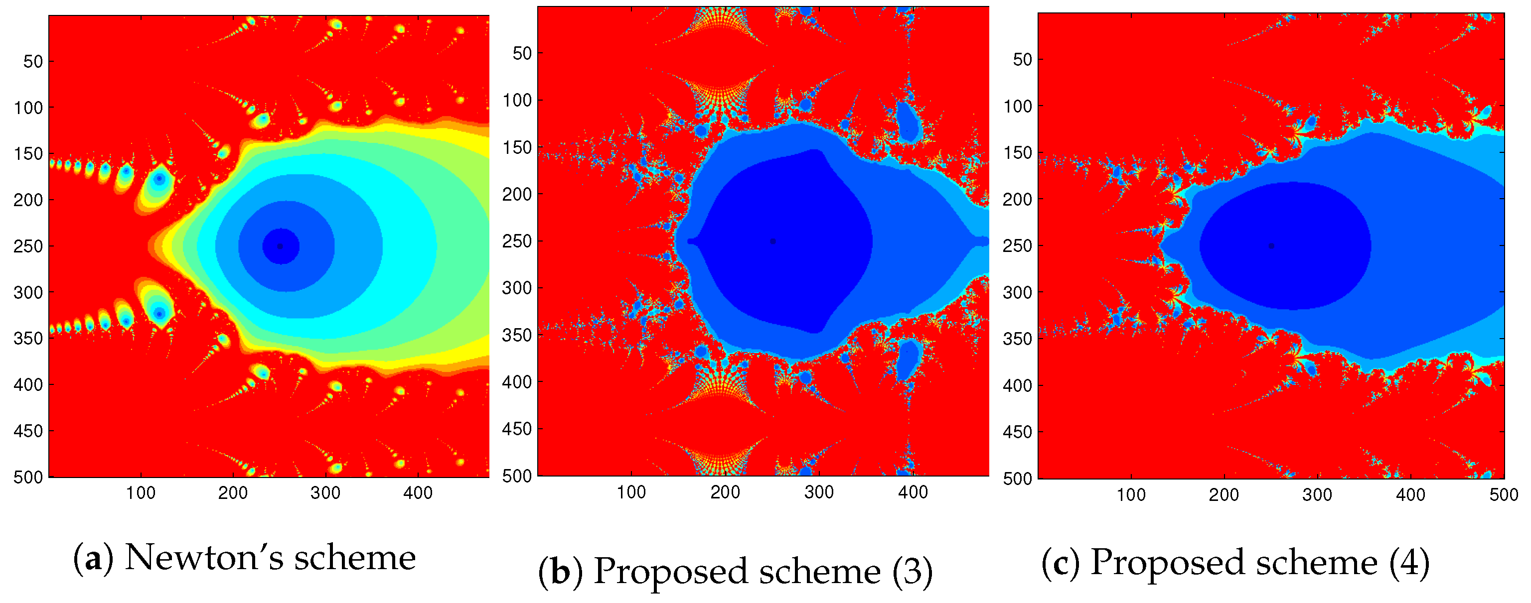
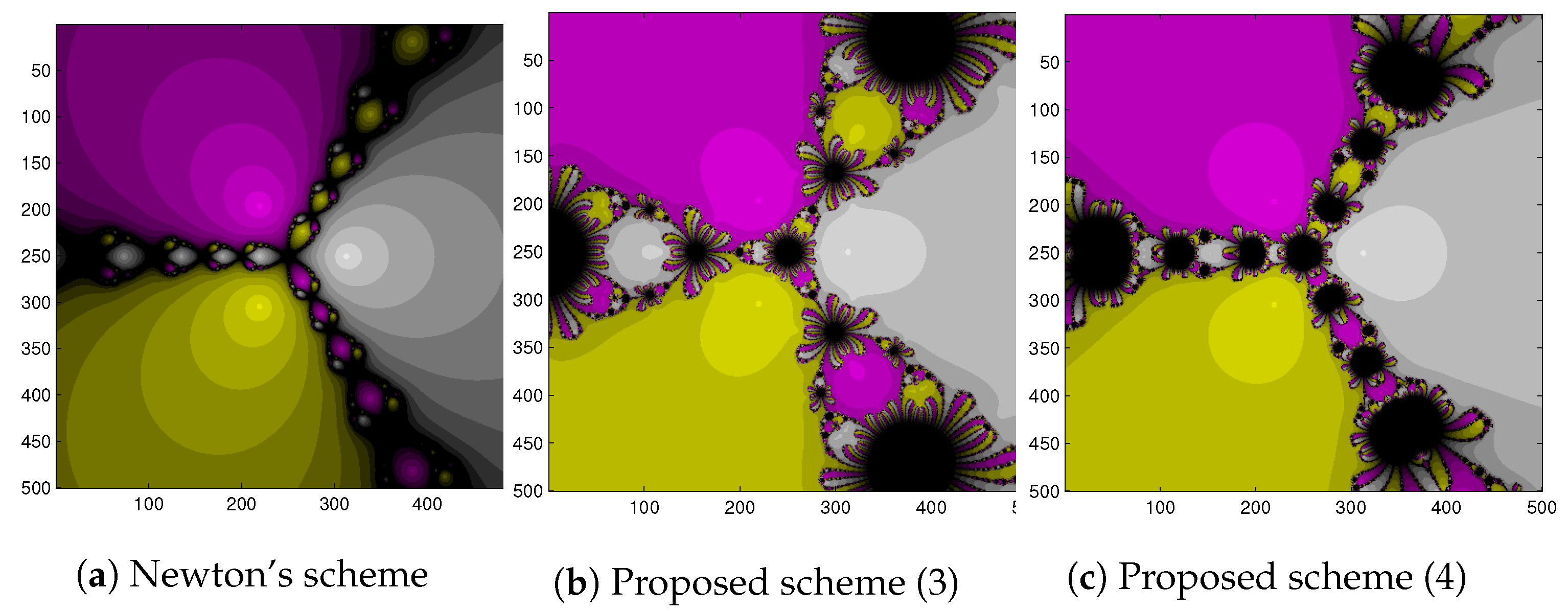
6. Dynamics of Scheme

We studied the dynamics and fractal patterns of the functions in example 1 $\left(F\right(z)=exp(z)-1)$ and example 2 ($F\left(z\right)=z^3-1$ ) by using proposed iterative schemes (3) and (4) along with Newton’s scheme. The dynamical analysis help us to study the convergence and stability of the schemes (see [6]).

6.1. For Example 1

We considered a square $R\times R=[-4.0,4.0]\times [-4.0,4.0]$ of $500\times 500$ points with a tolerance- $|f\left(z_n\right)|<5\times {10}^{-2}$ and a maximum of 11 iterations to study the dynamics of the function $F\left(z\right)=exp\left(z\right)-1$. We described the basins of attraction with a fixed color for the second-order Newton scheme, the ninth-order proposed scheme (3) and the ninth-order proposed scheme (4) for finding complex roots of the above-mentioned functions (Figure 1).

1.

The basins for all the iterative schemes contain a fractal Julia set and the basins of all the schemes look almost similar.

2.

The basins of attraction of the second-order Newton scheme contain a higher number of orbits and are less dark in comparison with the ninth-order schemes.

3.

Again, the Fatou set with blue color shows the basins of the schemes. The blue-colored area shows that the proposed scheme (4) contains the Fatou set with bigger and darker orbits.

6.2. For Example 2

We plotted the fractal pattern graph of example 2 ($F\left(z\right)=z^3-1$ ) for the different iterative schemes under the same previous conditions with a different color fixed to each root of the basins of attraction.

The basins of attraction for schemes to find the complex roots of example 2 ($F\left(z\right)=z^3-1$) are shown in Figure 2. We can see that there are no extraneous fixed points for the second-order Newton scheme, which is in agreement with the findings of the section Extraneous Fixed Points. Again, there are 106 extraneous fixed points for the proposed ninth-order scheme (3) and 129 extraneous fixed points for the proposed ninth-order scheme (4). Since, the magnitude of the derivative at these points is $>1$, these fixed points are repulsive. Thus, we see that scheme (3) is better in terms of extraneous fixed points.

7. Convergence Radii

In the next two examples, we compute the convergence radii for proposed schemes (3) and (4).

Example 5.

By the example in the Section 1, conditions (A) are satisfied if we choose $h_0\left(t\right)=h\left(t\right)=97t$ and $h_1\left(t\right)=2.$ Then, by solving the convergence radii, we have

$$r_1=0.010256678622334536$$

$$r_2=0.36382236284223446,0.0103087361577125$$

$$r_3=0.10153752845355392,0.22527857007361768,1.3993484775051468$$

$$r_4=0.11929997098554257,0.21910981171003618$$

and

$$\overline{r_1}=0.010256678622334536$$

$$\overline{r_2}=0.08299300112444563$$

$$\overline{r_3}=0.5291548166116622$$

$$\overline{r_4}=0.5420088529012402$$

Example 6.

Let $B_1$ and $B_2$ be the space of continuous functions on the interval $[0,1]$ with the max-norm and $\mathrm{\Omega }=\overline{S}(0,1)$. Define $F:\mathrm{\Omega }\to B_2$ by

$$F\left(\psi \right)\left(x\right)=\psi \left(x\right)-{\int }_0^{1}x\tau \psi {\left(\tau \right)}^{3}d\tau .$$

Then, the Fréchet derivative is given as

$$F\left(\psi \left(\mu \right)\right)\left(x\right)=\mu \left(x\right)-3{\int }_0^{1}x\tau \psi {\left(\tau \right)}^2\mu d\tau$$

for all $\mu \in \mathrm{\Omega }$. Then, conditions (A) are satisfied if we choose $h_0\left(t\right)=1.5t,h\left(t\right)=3t$ and $h_1\left(t\right)=2.$

Then, we have

$$r_1=0.4574271077563381$$

$$r_2=0.7496405298576232,0.46028836028846015$$

$$r_3=0.7444569229567777,0.5894382155567577,0.501131729398928$$

$$r_4=-0.6180132678614112$$

and

$$\overline{r_1}=0.4574271077563381$$

$$\overline{r_2}=0.8074036383761246,-0.7071105546988605,0.5879931572730634,0.486927560161037$$

$$\overline{r_3}=0.5291548166116622$$

$$\overline{r_4}=0.5420088529012402$$

8. Conclusions

We developed two ninth-order Newton-like schemes for solving nonlinear equations in Banach space and discussed the ball convergence analysis for both of them. We performed a local convergence comparison with the use of only the first-order derivative. The study is used to prove the convergence for scheme (3) and scheme (4) under weak conditions, extending the usage of these schemes. Earlier work relies on the existence and boundedness of $F^4$, which is not in these schemes. Thus, these results are not applicable in cases where these hypothesis are violated. However, these schemes may converge. We checked the theoretical results by using the numerical examples along with the boundary value problem. We also examined the numerical results with the basins of attraction for some selected examples. All the results (theoretical, numerical, dynamical) are generative for the advanced study of higher-order Newton-like schemes. The new approach is applicable in other schemes. This is revealing for our future research.

References

1. Singh, M.K. A Six-order variant of Newton’s method for solving non linear equations. Comput. Meth. Sci. Technol. 2009, 15, 185–193. [Google Scholar] [CrossRef]
2. Vrscay, E.R.; Gilbert, W.J. Extraneous fixed points, basin boundaries and chaotic dynamics for Schroder and Konig rational iteration functions. Numer. Math. 1987, 52, 1–16. [Google Scholar] [CrossRef]
3. Wang, K.; Kou, J.; Gu, C. Semilocal convergence of a sixth-order jarrat method in Banach spaces. Numer. Algorithms 2011, 57, 441456. [Google Scholar] [CrossRef]
4. Singh, M.K.; Singh, A.K. Variant of Newton’s Method Using Simpson’s 3/8th Rule. Int. J. Appl. Comput. 2020, 6, 20. [Google Scholar] [CrossRef]
5. Argyros, I.K. Convergence and Applications of Newton-Type Iterations; Springer: Berlin, Germany, 2008. [Google Scholar]
6. Argyros, I.K.; Magrenan, A.A. Iterative Methods and Their Dynamics with Applications: A Contemporary Study; Taylor and Francis: Boca Raton, FL, USA, 2017. [Google Scholar]
7. Cordero, A.; Torregrosa, J.R. Variants of Newton’s method using fifth-order quadrature formulas. Appl. Math. Comput. 2007, 190, 686–698. [Google Scholar] [CrossRef]
8. Grau-Sánchez, M.; Grau, A.; Noguera, M. On the computational efficiency index and some iterative methods for solving systems of nonlinear equations. J. Comput. Appl. Math. 2011, 236, 1259–1266. [Google Scholar] [CrossRef]
9. Homeier, H.H.H. A modified Newton method with cubic convergence: The multivariable case. J. Comput. Appl. Math. 2004, 169, 161–169. [Google Scholar] [CrossRef]
10. Homeier, H.H.H. On Newton-type methods with cubic convergence. J. Comput. Appl. Math. 2005, 176, 425–432. [Google Scholar] [CrossRef]
11. Jarratt, P. Some fourth order multipoint iterative methods for solving equations. Math. Comput. 1996, 20, 434–437. [Google Scholar] [CrossRef]
12. Kantorovich, L.V.; Akilov, G.P. Funtional Analysis; Pergamon Press: Oxford, UK, 1982. [Google Scholar]
13. Xiao, X.Y.; Yin, H.W. Accelerating the convergence speed of iterative methods for solving nonlinear systems. Appl. Math. Compt. 2018, 333, 8–19. [Google Scholar] [CrossRef]
14. Xiao, X.Y.; Yin, H. Achieving higher order of convergence for solving systems of nonlinear equations. Appl. Math. Compt. 2017, 311, 251–261. [Google Scholar] [CrossRef]
15. Cordero, A.; Torregrosa, J.R. Variants of Newton’s method for functions of several variables. Appl. Math. Comput. 2006, 183, 199–208. [Google Scholar] [CrossRef]
16. Sharma, J.R.; Guha, R.K.; Sharma, R. An efficient fourth order weighted-Newton method for systems of nonlinear equations. Numer. Algorithms 2013, 62, 307–323. [Google Scholar] [CrossRef]
17. Noor, M.A.; Waseem, M. Some iterative methods for solving a system of nonlinear equations. Comput. Math. Appl. 2009, 57, 101–106. [Google Scholar] [CrossRef]
18. Cordero, A.; Martínez, E.; Torregrosa, J.R. Iterative methods of order four and five for systems of nonlinear equations. J. Comput. Appl. Math. 2009, 231, 541–551. [Google Scholar] [CrossRef]
19. Sharma, J.R.; Gupta, P. An efficient fifth order method for solving systems of nonlinear equations. Comput. Math. Appl. 2014, 67, 591–601. [Google Scholar] [CrossRef]
20. Argyros, I.K. Computational Theory of Iterative Methods, Series: Studies in Computational Mathematics; Elsevier Publishing Company: New York, NY, USA, 2007. [Google Scholar]
21. Xiao, X.Y.; Yin, H.W. A new class of methods with higher order of convergence for solving systems of nonlinear equations. Appl. Math. Comput. 2015, 264, 300–309. [Google Scholar] [CrossRef]
22. Xiao, X.Y.; Yin, H.W. Increasing the order of convergence for iterative methods to solve nonlinear systems. Calcolo 2016, 53, 285–300. [Google Scholar] [CrossRef]
23. Sandor, K. Optimizing single Slater determinant for electronic Hamiltonian with Lagrange multipliers and Newton-Raphson methods as an alternative to ground state calculations via Hartree-Fock self consistent field. AIP Conf. Proc. 2019, 2116, 450030. [Google Scholar] [CrossRef]
Figure 1. Basin of attraction for e x p ( z ) 1 with different schemes.
Foundations 03 00039 g001
Figure 2. Basin of attraction for f 2 = z 3 1 with different schemes.
Foundations 03 00039 g002