
Hydroxyl Spectroscopy of Laboratory Air Laser-Ignition

Physics and Astronomy Department, University of Tennessee, University of Tennessee Space Institute, Center for Laser Applications, 411 B.H. Goethert Parkway, Tullahoma, TN 37388-9700, USA
Foundations 2022, 2(4), 934-948; https://doi.org/10.3390/foundations2040064
Submission received: 12 September 2022
/
Revised: 14 October 2022
/
Accepted: 14 October 2022
/
Published: 18 October 2022
(This article belongs to the Special Issue Advances in Fundamental Physics II)
Abstract
:This work investigates spatial and temporal distributions of hydroxyl, OH, in laser-plasma in laboratory air at standard ambient temperature and pressure. Of interest are determination of temperature and density of OH and establishment of a correlation of molecular OH emission spectra with shadow graphs for time delays of 50 to 100 μs, analogous to previous work on shadow graph and emission spectroscopy correlation for cyanide, CN, in gas mixtures and for time delays of the order of 1 μs. Wavelength- and sensitivity-corrected spatiotemporal data analysis focuses on temperature inferences using molecular OH emission spectroscopy. Near-IR radiation from a Q-switched laser device initiates optical breakdown in laboratory air. The laser device provides 6 ns, up to 850 milli Joule, pulses at a wavelength of 1064 nm, and focal irradiance in the range of 1 to 10 terawatt per centimeter-squared. Frequency doubled beams are utilized for capturing shadow graphs for visualization of the breakdown kernel at time delays in the range of 0.1 to 100 μs. OH emission spectra of the laser plasma, spatially resolved along the slit dimension, are recorded in the wavelength range of 298 nm to 321 nm, and with gate widths adjusted to 10 μs for the intensified charge-coupled device that is mounted at the exit plane of a 0.64 m Czerny-Turner configuration spectrometer. Diatomic OH signals occur due to recombination of the plasma and are clearly distinguishable for time delays larger than 50 μs, but are masked by spectra of N2 early in the plasma decay.
1. Introduction
Hydroxyl, OH, spectroscopy shows applications in diverse research endeavors including plasma physics, analytical chemistry, astrophysics, and obviously, in combustion physics and associated combustion chemistry [1,2,3,4,5,6]. The astrophysics OH interest [5] led to the first hydroxyl radical detection in the near infrared emission spectra of an exoplanet atmosphere. The work presented in this paper is centered on the near-uv spectra of OH in laser-plasma, yet combustion diagnosis of hydrogen flame temperatures in a research rocket combustor may focus on hyperfine structure with experimental resolution of 50 pm for OH-radical fingerprints [6]. The experimental component initiates laser-plasma [7,8,9,10] in standard ambient temperature and pressure (SATP) laboratory air. The analysis component utilizes line strength data that show an accuracy of better than one-thousandth of a nanometer (nm) or 1 picometer (pm) [11] with a typical laser-plasma experiments instrumental resolution of 0.35 nm, or 350 pm [11,12].
The primary reason for occurrence of OH is the presence of moisture in SATP air. However, OH emission signals show spectroscopic interference from the N2 Second Positive system that usually occurs in nitrogen discharges [13]. Recorded spectra in air breakdown dwarf signal strengths that can be measured in combustion processes that utilize oxygen as oxidizer, for example, combustion of hydrocarbons [14,15]. However, when exploring combustion and laser-plasma in gases, usually strong signals define the spectroscopy of emanating light with notable contributions of diatomic carbon (C2) Swan bands, cyanide (CN), and atomic signatures of the hydrogen Balmer series, e.g., hydrogen-beta line [16,17,18,19,20,21]. Laser-plasma in air, and for the wavelength range of 298 nm to 321 nm, reveals significant contributions from the N2 Second Positive system of nitrogen at time delays of typically 10 to 30 μs after optical breakdown [11,12], and OH emission signals are clearly discernible in the time delay range of 50 μs to 110 μs. Spatiotemporal information is obtained by utilizing the slit dimension for the spatial resolution. The temporal resolution is obtained from a systematic set of time delays that are selected for an intensified charge-coupled device (ICCD) mounted at the exit plane of a spectrometer. The experimental methodology, including choice of laser-plasma generation by aligning beam propagation and focusing parallel to the slit, is analogous to that designed for recent cyanide, CN, diatomic molecular studies [22]. The shadow graphs are recorded by employing a digital camera, thereby allowing one to associate spatial connections with the time-resolved, recorded spectra. The concentration of OH molecules is inferred from equilibrium species distributions computations that employ freely available code for chemical equilibrium with applications [23,24].
2. Materials and Methods
The experimental arrangement for recording of spatiotemporal molecular distributions has been communicated previously. however, for completeness it is included in this work. The standard experimental components are used for laser-induced breakdown spectroscopy and have been summarized previously, e.g., see Ref. [11].
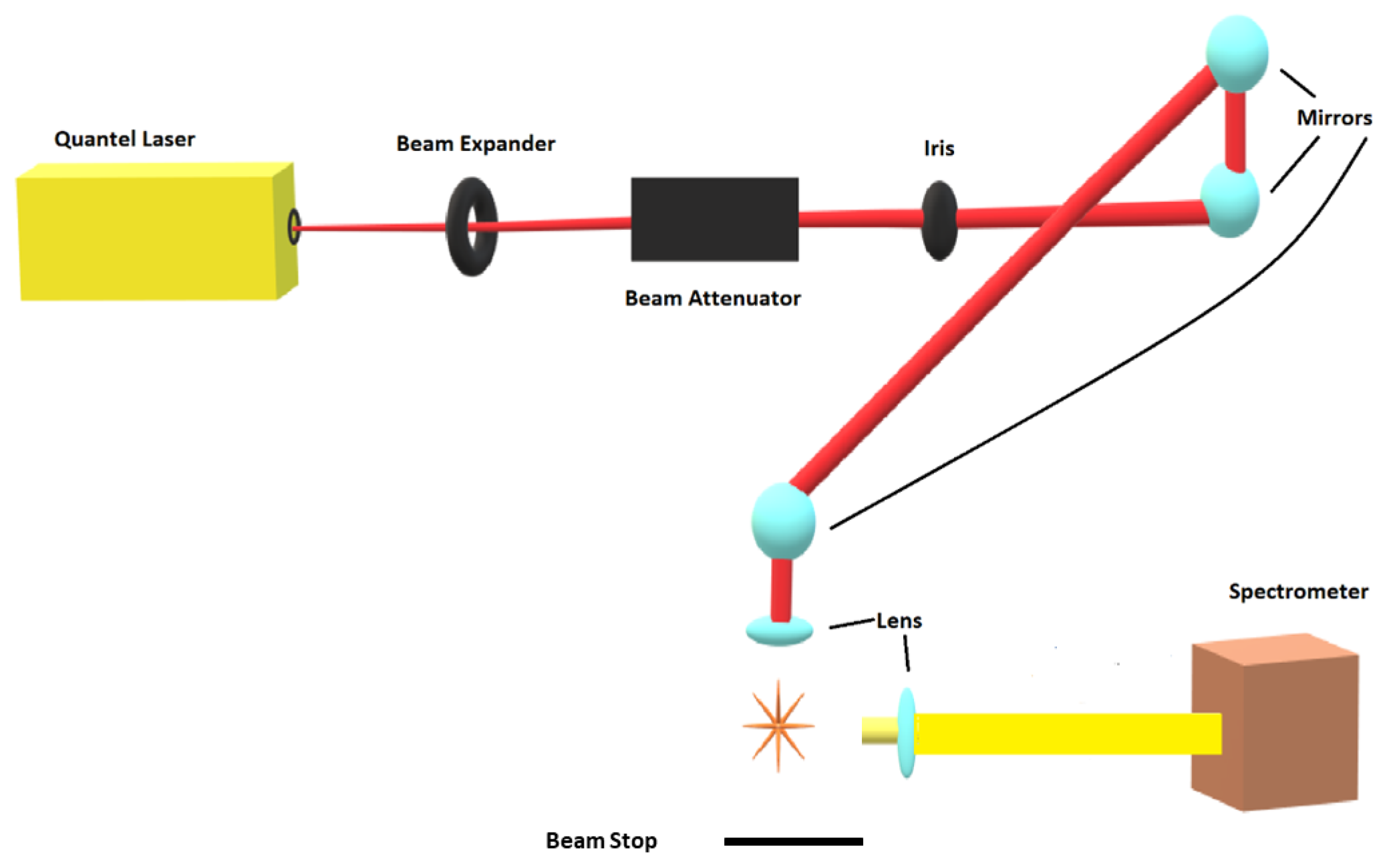
The experimental arrangement consists of a set of components typical for time-resolved, laser-induced optical emission spectroscopy, or nanosecond laser-induced breakdown spectroscopy (LIBS). Figure 1 displays the principal schematic of the experimental arrangement.
Primary instrumentations include a Q-switched Nd:YAG device, Quantel model Q-smart 850, operated at the fundamental wavelength of 1064-nm to produce full-width-at-half-maximum 6-ns laser radiation with an energy of up to 850 mJ per IR pulse, a laboratory type Czerny–Turner spectrometer, Jobin Yvon model HR 640, with a 0.64 m focal length and equipped with a 1200 grooves/mm grating, an intensified charge-coupled device, Andor Technology model iStar DH334T-25U-03, for recording of temporally and spatially resolved spectral data, a laboratory chamber or cell with inlet and outlet ports together with a vacuum system, electronic components for synchronization, and various optical elements for beam shaping, steering and focusing. For 1:1 imaging of the plasma onto the 100 μm spectrometer slit, a fused silica plano-convex lens, Thorlabs model LA4545, is employed. For the OH experiments, the laser pulse energy is attenuated with beam splitters and apertures from 850 to 170 mJ/pulse. The residual, transmitted laser pulse is captured by the beam stop that is indicated in Figure 1.
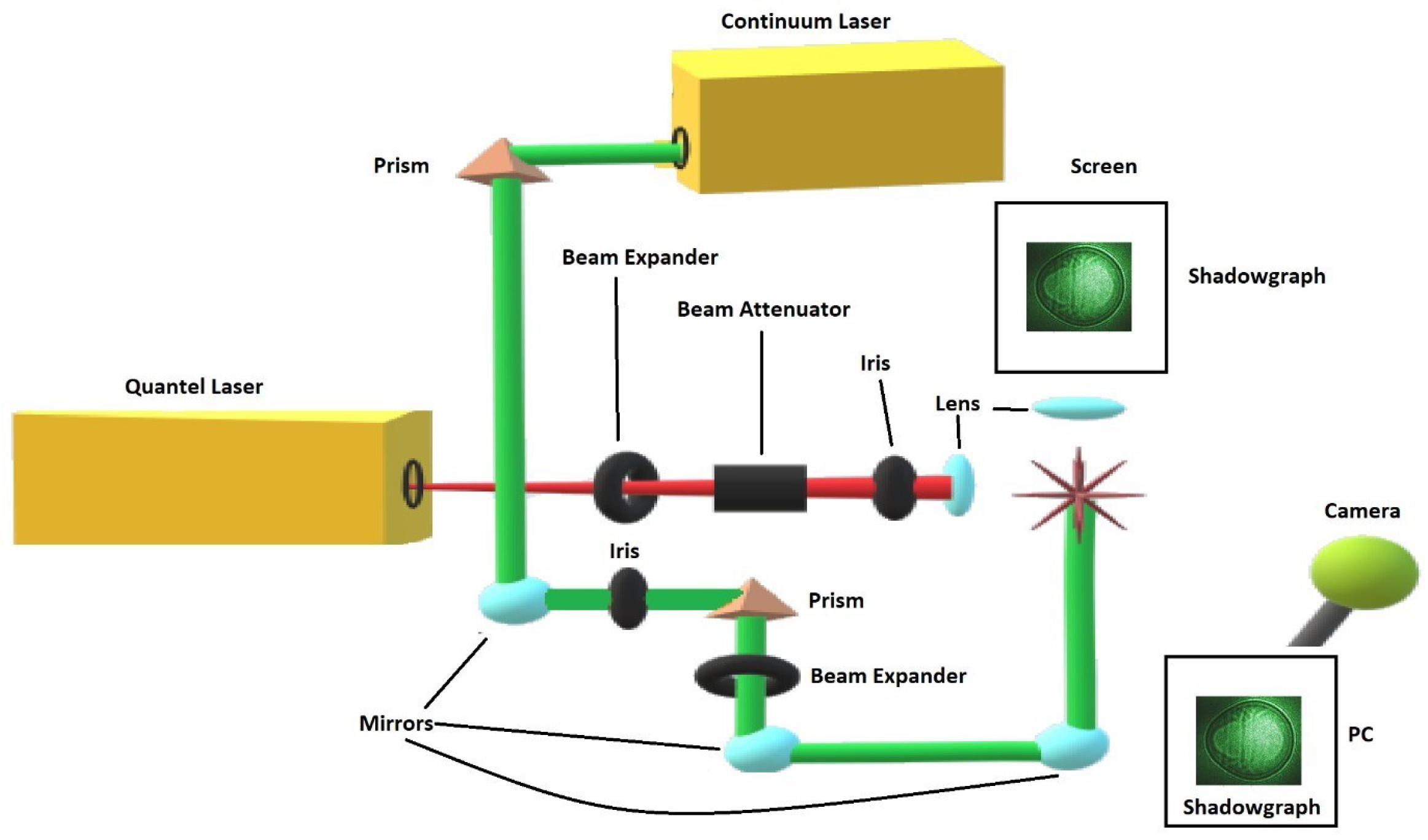
For visualization studies reported here, a separate laser device, Continuum Surelite model SL I-10, delivers two frequency-doubled beams at the 2nd harmonic, 532-nm wavelength, and both breakdown and shadow graph beams are spatially overlapped. The pulses for shadowgraphy can be delivered with a minimum time delay of 300 ns and with a well defined time delay showing less than ±1 ns trigger-jitter between the pulses. Shadow graphs are recorded by external synchronization of the Surelite and Quantel laser devices and by externally triggering the camera, a Silicon Video 9C10 color camera, that records the images that are projected onto a screen. Single-event shadow graphs were captured independent from the measurements of optical breakdown spectra. The color camera shows 3488 width- × 2616 height-pixels, but for the shadow graphs the pixels were grouped in 4 × 4 pixel packets. Furthermore, the width to height was adjusted to 600 × 500 for these 4 × 4 pixel packets. Consequently, displayed shadow graphs, e.g., would on average cover ≃12 μm × 12 μm per 4 × 4 pixel packet. Figure 2 illustrates the modular setup for recording of shadow graphs.
In studies with time-resolved spectroscopy, optical breakdown at a rate of 10 Hz was generated by focusing from the top (see Figure 1) the expanded laser beam with f/5 optics with an anti-reflection coated, 25.4-mm (1 in.) lens, or parallel to the slit, analogous to recently reported CN laser spectroscopy [22]. The air-breakdown plasma is imaged 1:1 with a 50.8-mm lens. Time-resolved data are recorded with an intensified charge-coupled device positioned at the exit plane of the spectrometer.
In the experiments, the irradiance is of the order of 10× more than that needed for optical breakdown in dry air [25]. However, from CO2 laser breakdown investigations, the breakdown threshold in the moist air troposphere can exceed that of dry air by 20 to 30 percent [26]. A similar breakdown increase is inferred for 1064-nm Nd:YAG radiation and for 25% humidity during the experimental data collection. The detector pixels are grouped together in four-pixel tracks with a total linear dimension of 54 μm along the slit direction, resulting in obtaining 256 tracks covering 13.8 mm for each time delay. Typically, 4 mm of the central third of the four-pixel tracks of the detector recorded OH spectra, showing a spatial resolution of ∼54 μm each for ∼75 tracks when assuming perfect vertical mapping of spectrometer input (slit) to output plane (detector). Measurements comprise accumulation of 100 consecutive laser-plasma events for 11 separate time delays at 10 μs steps with a 10 μs gate centered at the selected time delay. The selected series explores the plasma decay with specific attention to recognition of OH molecular data that are free from spectroscopic interference. However, the 0-0 OH band edge is marginally recognizable for time delays of 10 μs and 20 μs, but almost N2 interference-free data are captured for time delays as early as about 50 μs.
Computation of hydroxyl spectra utilizes well-established line-strength data for the diatomic OH molecule. Application of standard quantum mechanics establishes within the concept of line strengths [27] consistent computation of diatomic spectra. The OH line-strength data are published as a supplement to a recent paper on hydroxyl [11]. However, an abridged data file containing sets of three values, i.e., transition wave numbers, lower-level term values, and transition-strengths, is sufficient for routine computation of diatomic OH spectra using widely available MATLAB software [28] and convenient scripts [29] for computation of spectra and for fitting of recorded spectra.
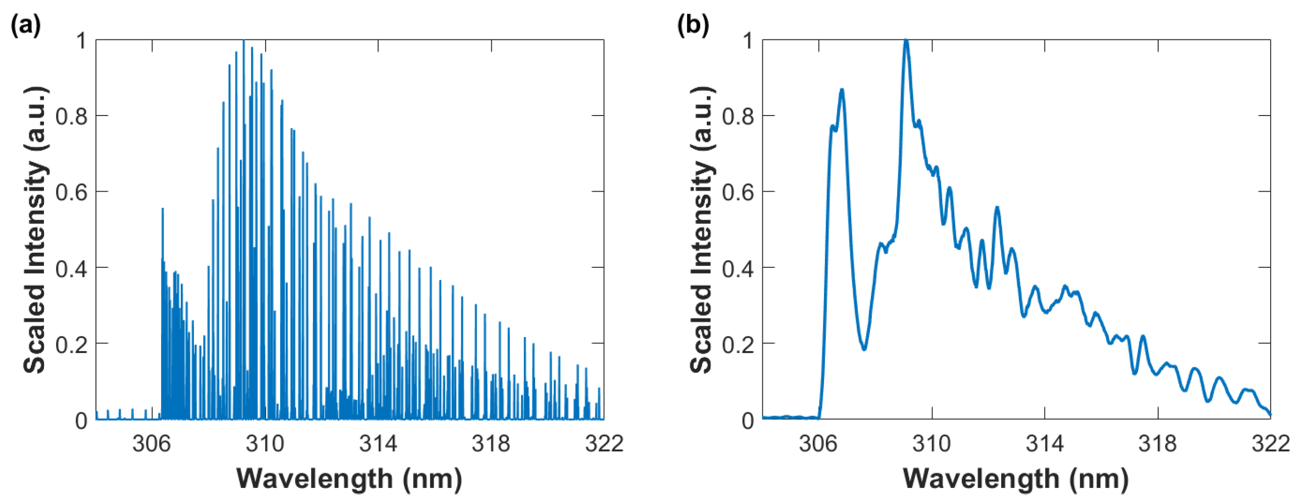
Figure 3 illustrates computed OH data using the MATLAB BESP.m script [29] for spectral resolutions of 0.001 nm and 0.35 nm, the latter corresponds to a typical resolution in laser-induced spectroscopy with intensified array detectors and the former is used for nominal pico-meter resolution stick-spectra. OH spectra in the indicated 304 nm to 322 nm wavelength range clearly show the 0-0 band edge near 306 nm of the red shaded A X ultraviolet system, the 1-1 band edge is near 312 nm, and the 2-2 band edge near 318 nm [11].
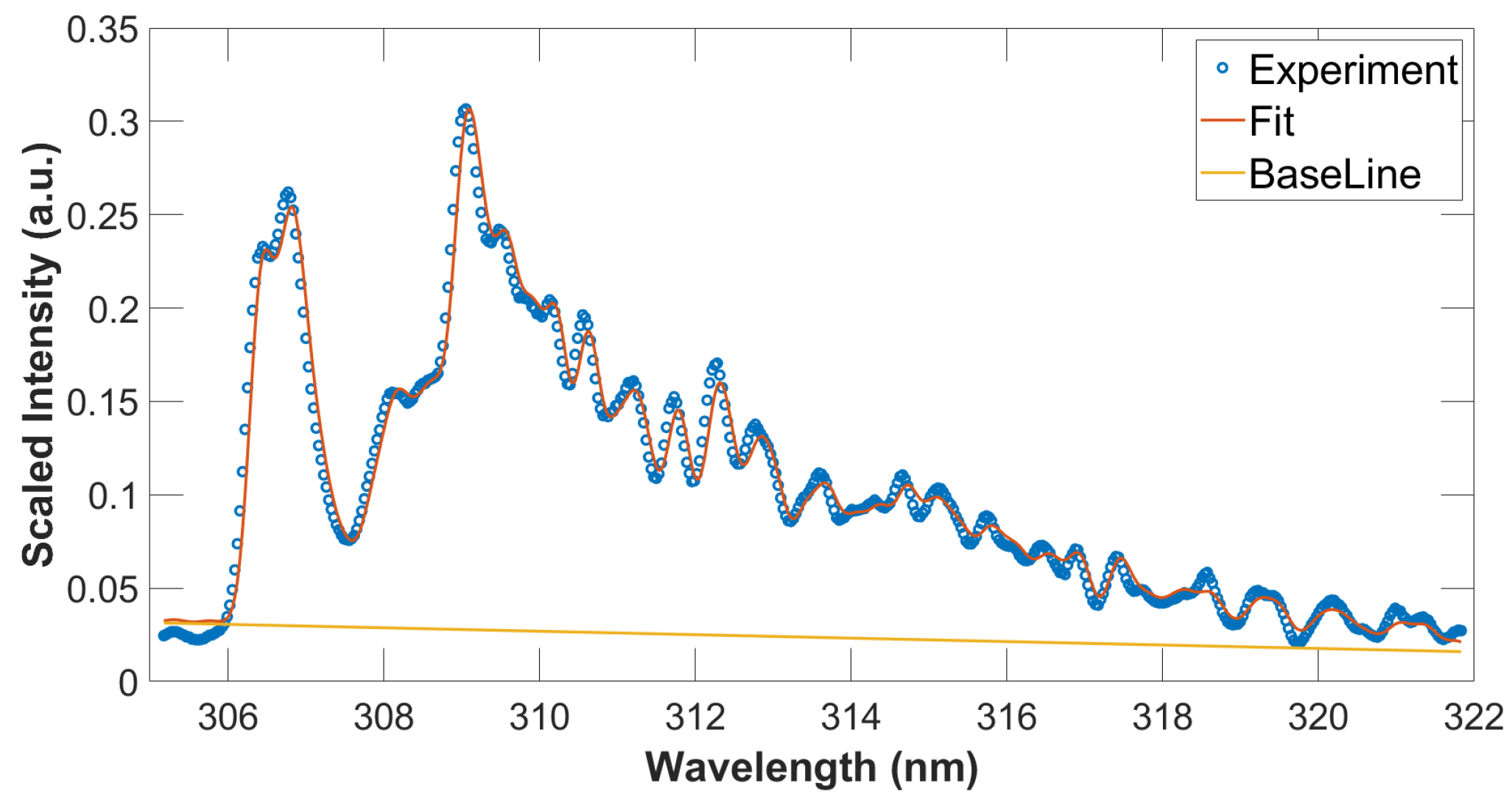
For the OH analysis, the MATLAB NMT.m script [29] was utilized. This particular script allows one to fit measured to computed data employing the Nelder–Mead nonlinear fitting algorithm. As an example, previously measured and communicated data [11,12] are analyzed for determination of temperature using MATLAB. Figure 4 displays the results, consisted with previous temperature inferences [16,17] with temperature errors of the order of 1 percent obtained by Monte Carlo simulations when assuming random 10 percent spectral data variations for each wavelength position.
The calculation of the spectra relies on the use of OH line strength data [11]. Computation of diatomic spectra utilizes high resolution data for determination of molecular constants of selected molecular transitions from an upper to a lower energy level. Numerical solutions of the Schrödinger equation for potentials yield r-centroids associated with vibrational transitions usually involving Frank-Condon factors. Calculated rotational factors are interpreted as selection rules because these factors are zero for forbidden transitions, viz. Hönl-London factors.
3. Results and Discussion
3.1. Shadow Graphs
Investigations of expanding laser-induced shockwaves and fluid-physics phenomena utilize effectively high shutter-speed shadow graph photography. Figure 5, Figure 6 and Figure 7 display selected shadow graphs for time delays in the range of 0.1 μs to 104.25 μs.
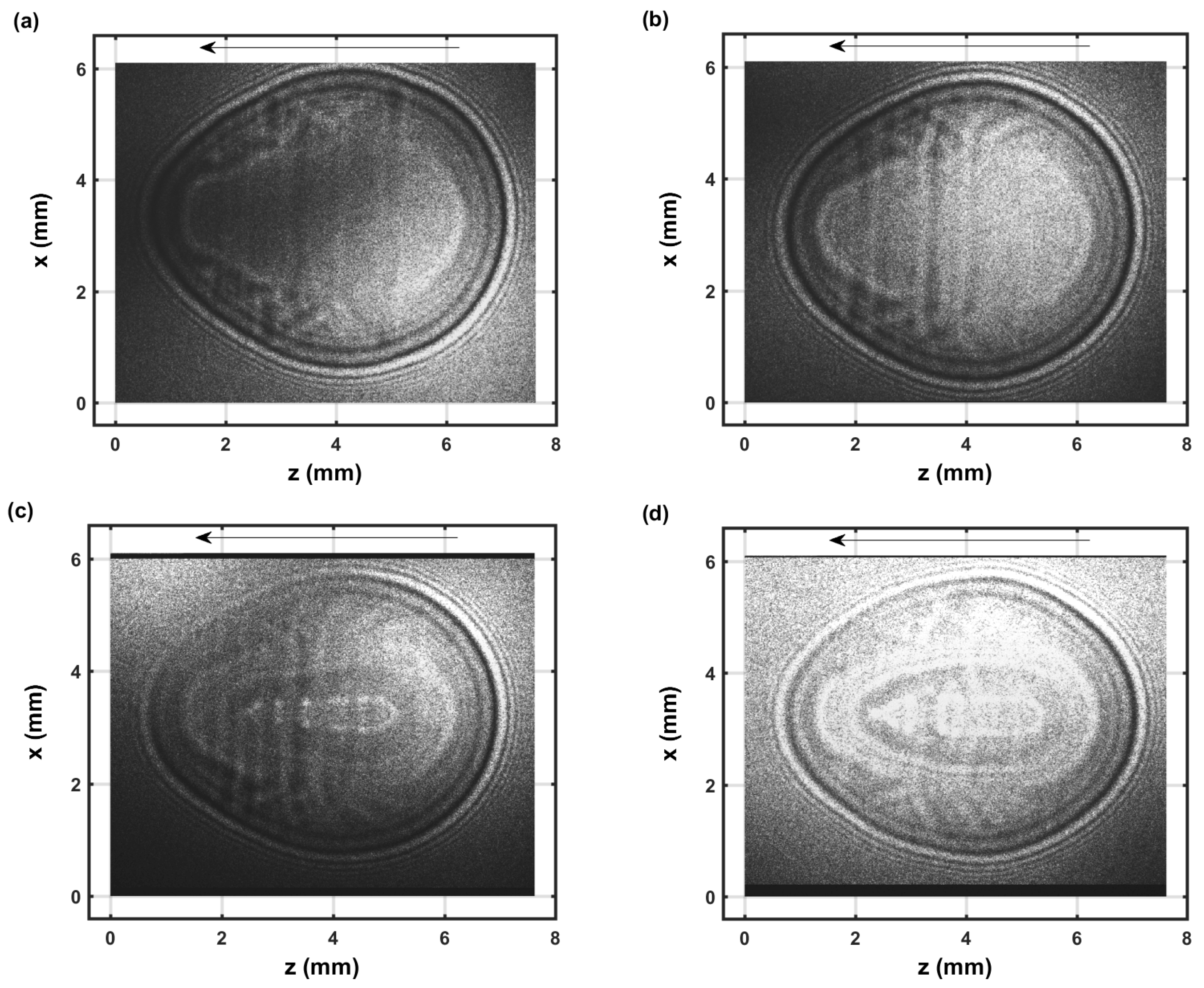
The IR laser beam is focused from right to left as indicated by the arrow in the images. The shock wave appears nearly symmetrical for the 1.15 μs images, see Figure 5, that evolved from a spheroidal image captured for time delays of 0.1 μs. In the 0.1 to 1 μs range, CN recombination spectra are measured [22]. The species density increase of electrons and diatomic molecular CN near the shockwave can be determined using Abel integral inversion [22]. The dark, close to spherically symmetric ring near the edges of the images for the 1.15 μs time delay shadow graph, see Figure 5a,b, corresponds to the radius of the shockwave, with minor dark/bright diffraction rings due to the use of a coherent back-light for shadowgraphy. The dark spheroidally shaped edge of >0.1 mm in the double exposure images and for 0.1 μs time delays, see Figure 5c,d, would indicate an expansion speed >20 km/s during the 5-ns pulse width of the back-light laser beam. From CN spectroscopy and for ∼1 μs time delay, one can infer that the primary dark/bright section corresponds to higher species density than inside and outside of the shock wave. Similarly, this work on OH spectroscopy indicates that the primary dark sections for ∼50 to 100 μs time delays correspond as well to higher species density than in the nearby regions.
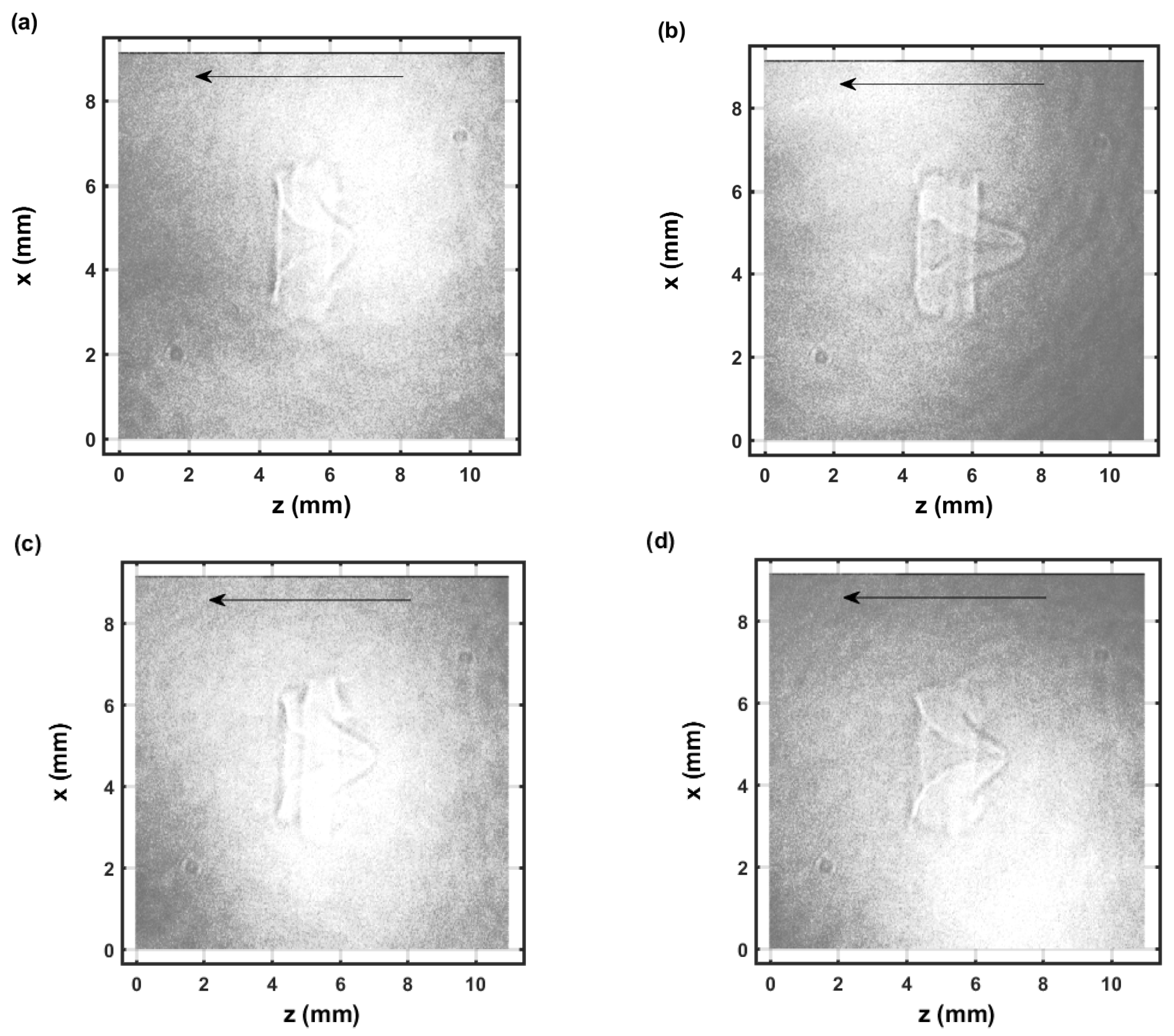
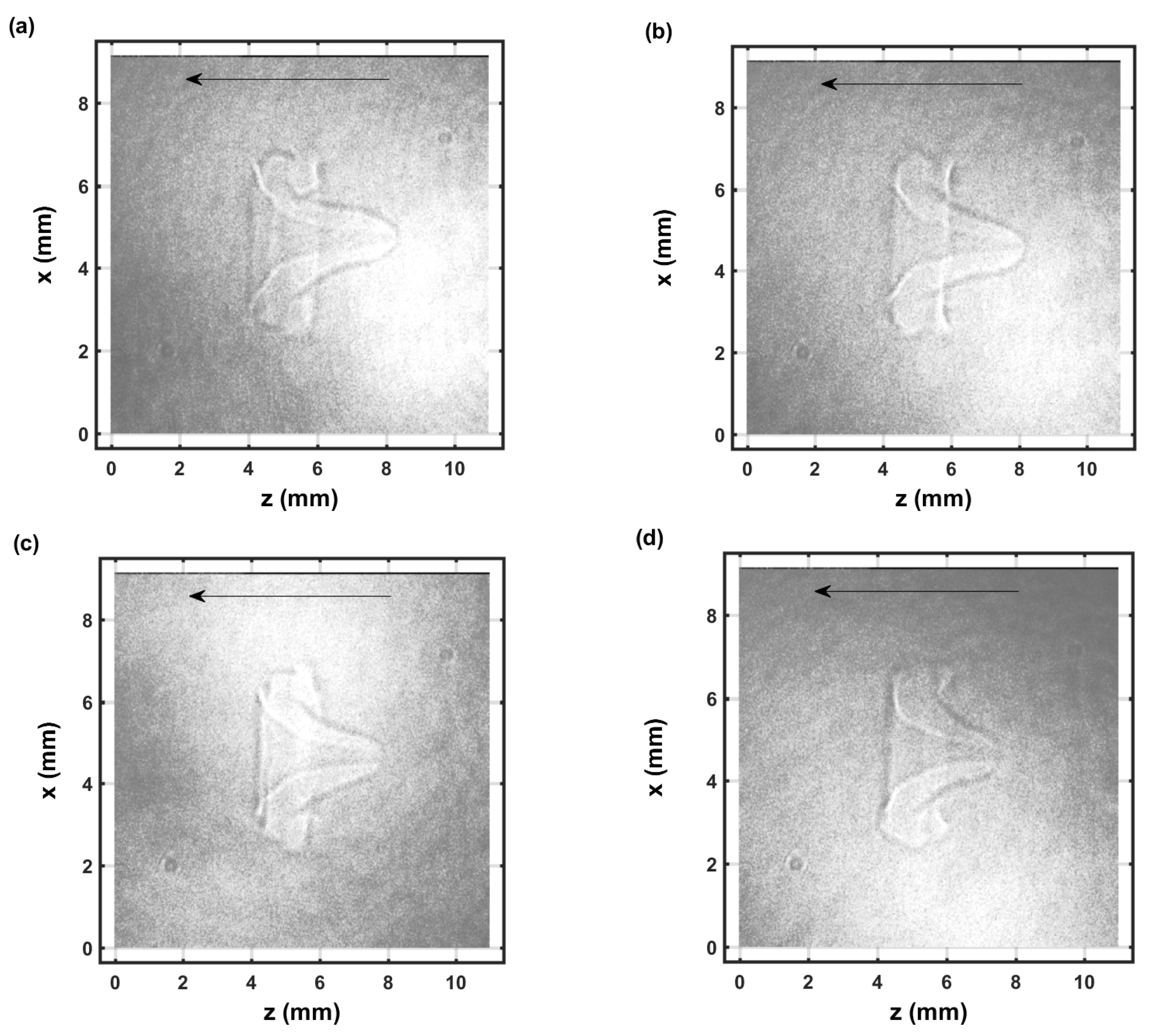
Figure 6 and Figure 7 illustrate selected shadow graphs for time delays of 54.25 μs and 104.25 μs, respectively. Well-developed vortices and fluid flow occur towards the incoming laser beam. The captured images for 54.25-μs time delays (Figure 6) appear to show slightly more apparent variations than those for 104.25-μs time delays (Figure 7). However, spatial variations are not obvious in the measured spatiotemporal OH spectra that are communicated in the next section.
In view of laser spectroscopy, time-resolved data taken for a narrow slice along the direction of the laser beam would be affected by fluid dynamics. By comparison, Figure 5 indicates close to spherical symmetry allowing one to utilize Abel inverse transform algorithms [22]. Spectroscopic diagnosis and correlation with the shadow graphs of Figure 6 and Figure 7 is expected to require simultaneous measurements in multiple or at least two directions, in other words, desirable is a computed tomography approach that utilizes Radon inverse transform [30,31,32]. For the employed experimental arrangement, integration occurs along the line-of-sight causing ambiguities in inferences of densities for obviously non-spherical expansion. However, the overall fluid expansion has been measured and computed previously in combustion research along with experimental studies utilizing planar laser-induced fluorescence [14,15].
3.2. Emission Spectra
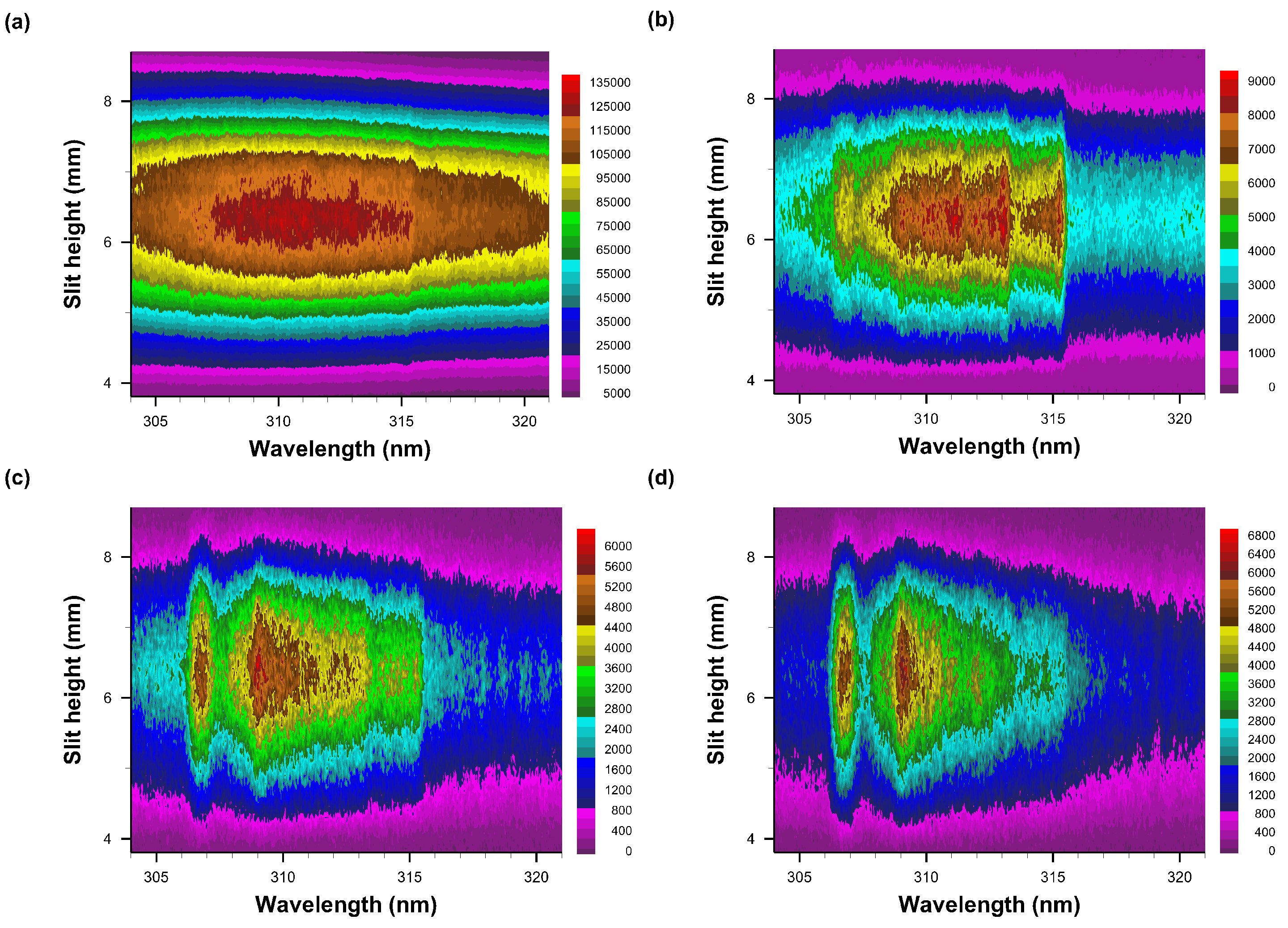
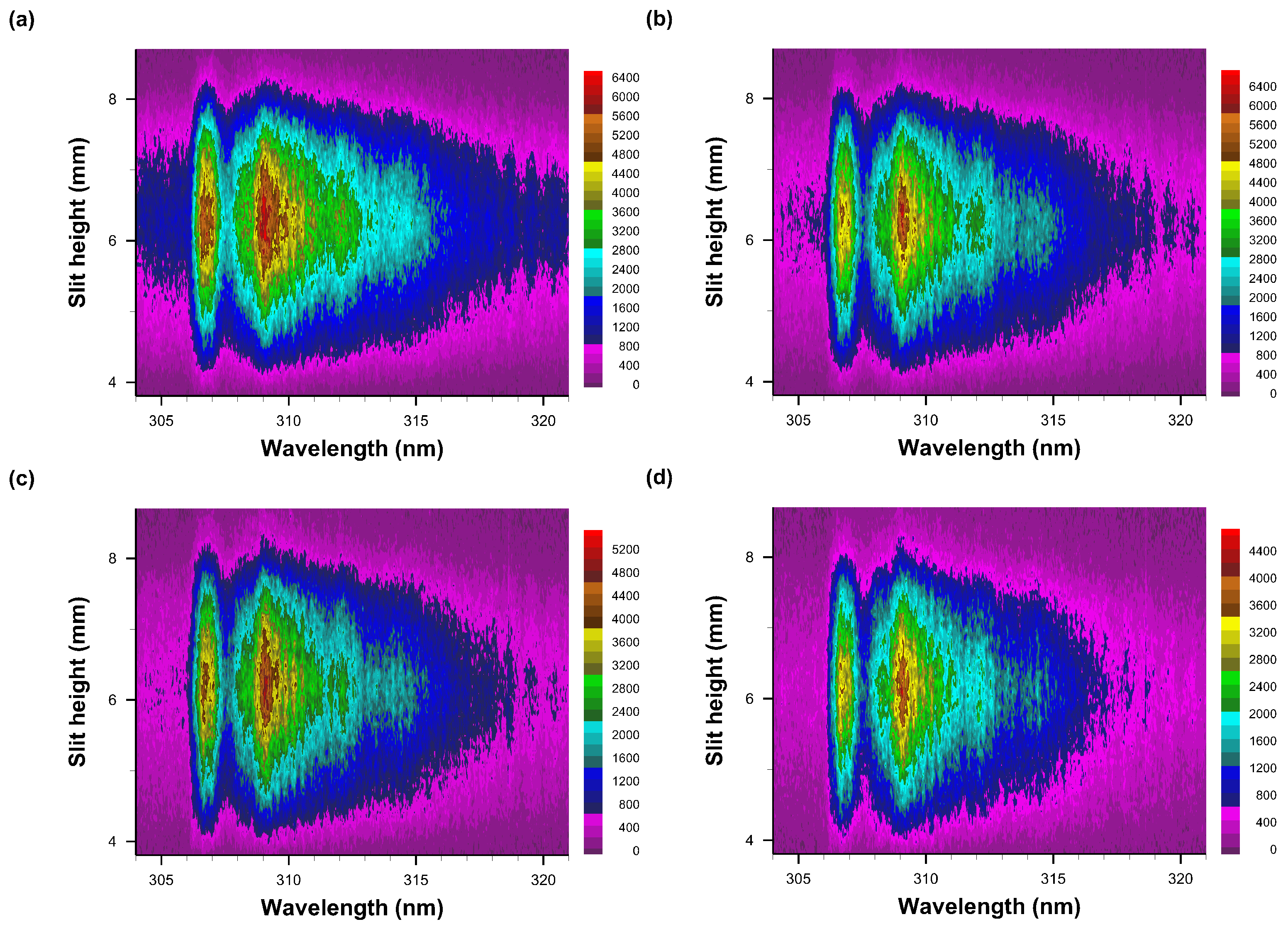
Figure 8, Figure 9 and Figure 10 illustrate recorded emission spectra along the slit height and in the range of 304 nm to 321.3 nm, and for time delays of 10 μs to 110 μs in 10 μs steps. All images are individually scaled from measured intensity (detector counts) minimum to maximum and processed for pseudo-color display.
The intensified detector has the capability of recording 1024 spatially resolved data, however, 4 pixels along the slit dimension, i.e., vertical, are grouped together for increased sensitivity of the actually recorded 256 spectra. The figures illustrate reasonable integrated signals from 100 consecutive laser-plasma events that are dispersed in approximately 100 spectra in the central region of the detector. Figure 8a displays faint N2 Second Positive band-edge signals near 315 nm, but Figure 8b reveals the OH A-X 0-0 band edge near 306 nm together with well demarcated N2 signals. Figure 8c,d depict how N2 signals diminish as OH becomes apparent.
Experimental averaging over 100 consecutive laser-plasma events enhances the signal to noise ratio by one order of magnitude. Conversely, as one collapses the 1024 vertical pixels to a single super-pixel, one mimics a linear diode array capable of recording single-shot OH spectra in laboratory air. Inspection of the spectra reveals that there is a slight curvature that would cause decreased resolution when averaging the central spectra.
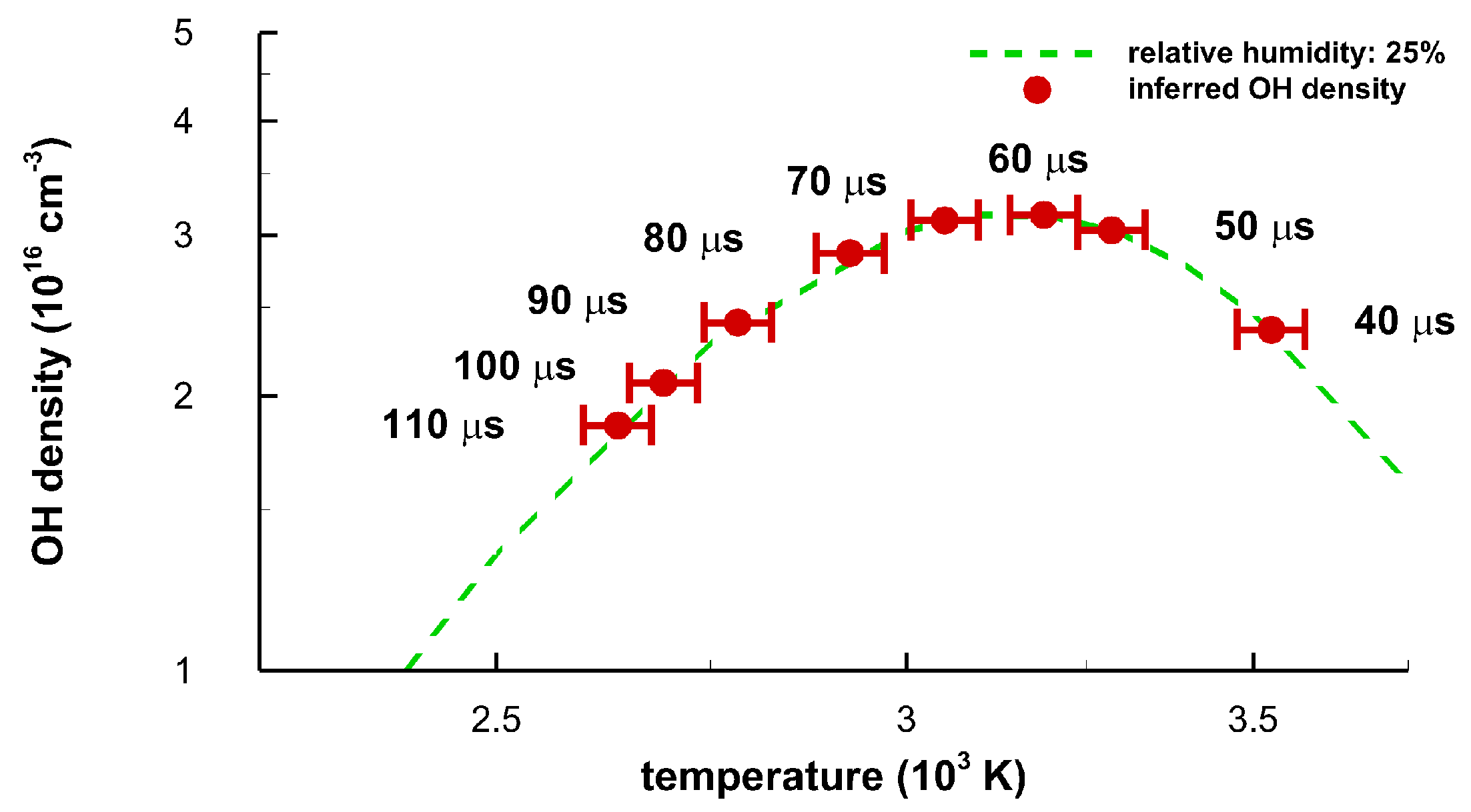
Figure 9a,b indicate similar, OH-band integrated signals or close to maximum OH signals as function of temperature if one computes the equilibrium species density v. temperature [11] and for a measured level of humidity. For air with 25% relative humidity, the OH density reaches a maximum of ≃3 × 1016 cm−3 at a temperature of T ≃ 3100 K.
Figure 10 illustrates the persistence of OH emission spectra for time delays of 90 μs to 110 μs, including two resolved peaks near the A-X 0-0 OH band edge that can be seen for an experimental spectral resolution of 0.35 nm.
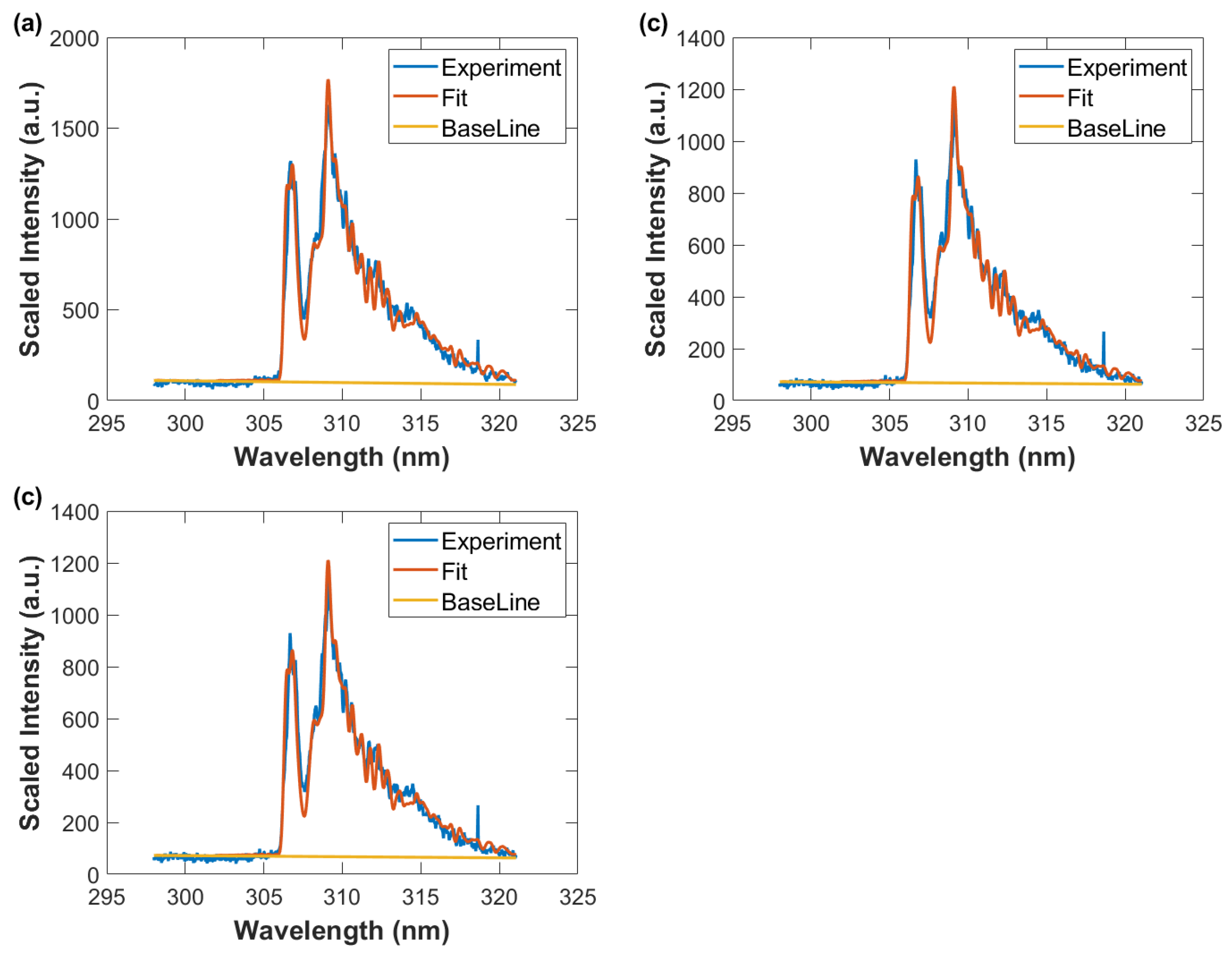
Measurement of OH in moisture-laden laboratory air can be accomplished at the single-shot level as elaborated above, i.e., when grouping together all vertical bins, thereby simulating a linear diode array. Figure 11, Figure 12 and Figure 13 display averages of the 5.44 mm central portion of the spatiotemporal data in Figure 8, Figure 9 and Figure 10.
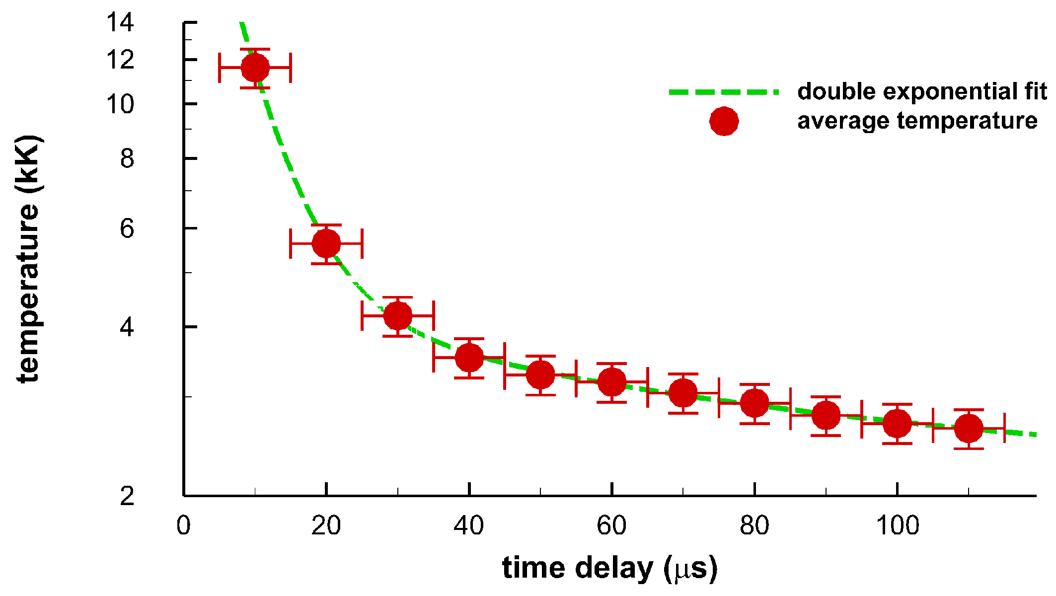
Figure 14 illustrates inferred temperatures from averages of wavelength calibrated and sensitivity corrected data in Figure 11, Figure 12 and Figure 13 of the displayed images in Figure 8, Figure 9 and Figure 10. The fitting procedures uses the Nelder–Mead algorithm and OH line-strength data for spectra fitting with constant instrument resolution of 0.35 nm and allowing a straight line background correction as well. The quoted instrument resolution is associated with the center wavelength of the displayed data. OH line strength data are utilized in terms of transition and lower term value wave-numbers that are adjusted to air wavelengths in the fitting program. For the 10-μs time-delay data, the temperature is estimated to be 1 eV, or 11,600 K, guided by Wien’s displacement law [33],
Wien’s displacement constant equals, , indicates the peak of the spectral radiance of black-body radiation, and T is the absolute temperature.
The double exponential fit, Figure 14, utilizes the MATLAB fit.m function to parameters a, b1, c1, b2, c2, for the function . The fitting routine finds the respective values of 2.14, 31.7, 0.146, 2.41, 0.0144, when using kK and μs units in the fitting routine. From Figure 10a, one would infer from Equation (1) a temperature of 9350 K. However, diatomic spectra of OH and N2 second positive are already developed. Consequently, the temperature is estimated to be higher than indicated by the peak in the 10-μs average data. Temperatures for the 20 μs to 110 μs data range are inferred from only fitting OH. The temperature error bars indicate an estimated experimental range of ±8 percent. However, further analysis with Monte Carlo simulations with random variations of the order of 10 percent along the lines discussed in Refs. [16,17] is expected to yield 1 percent error margins for OH spectra that show little or no spectral interference from other species, viz for time delays of the order of 100 μs [16,17]. The horizontal error bars indicate the gate-width of 10 μs.
3.3. Correlation of OH Emission Spectra and of Shadow Graphs
The recorded optical emission data of OH are difficult to connect with the measured shadow graphs [11]. However, expansive analysis of spatiotemporal data allows one to establish initial connections. First, average temperatures are associated with the equilibrium OH density for the spatiotemporal data, and second, spatially resolved temperatures are associated with OH density variations indicated in the shadow graphs.
The equilibrium OH concentrations are computed from the mole fraction data for the experiments in SATP laboratory air. The CEA program computes a volley of species for equilibrium conditions. Table 1 shows all species for selected temperatures in the range of 2500 K and 3750 K. The OH mole fraction peaks at 3144 K, and the OH mole fraction ratio at 6000 K and at 3100 K would amount to 3.6 × 10⁻³.
Figure 15 displays equilibrium OH density versus temperature for the majority of the time-delays selected in the experiment. The OH concentration is computed using the program for chemical equilibrium with applications [23,24]. The ±8 percent temperature error bars are shortened to ±1.5 percent for the purpose of readability. However, Monte Carlo simulations, for the purpose of estimating error bars with a random error magnitude of 0.1 to 0.2 of the mean spectral data recorded with a linear diode array, revealed 1 to 2 percent variations of temperature inferred from OH spectra that show minimal interference from other species in previous air breakdown studies [16,17]. It would be expected that a similar numerical analysis would show temperature error bars of the order of 1 percent.
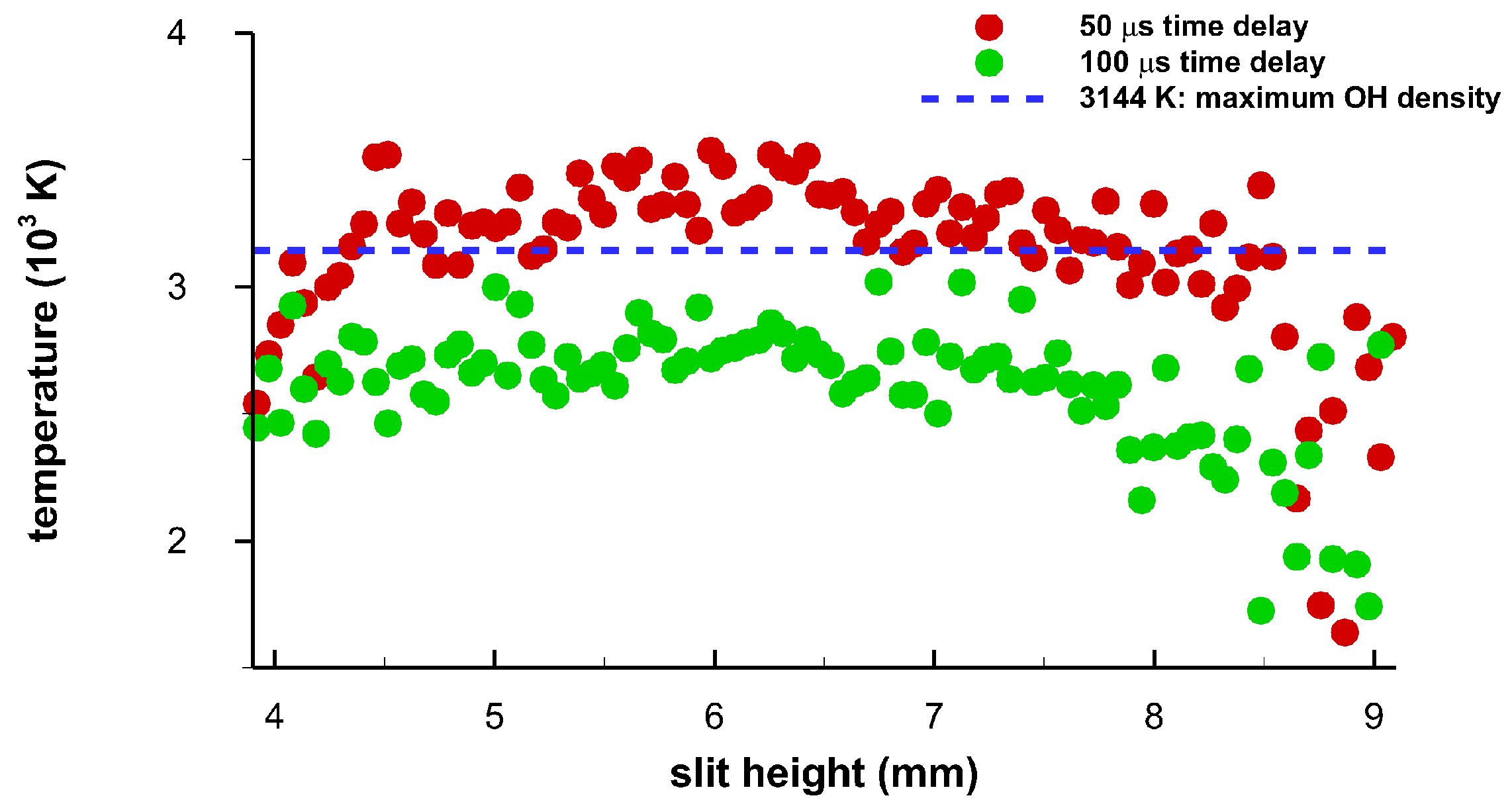
Analysis of the 1100 spectra in the central region of the 2816 captured spatially- and temporally-resolved data reveals subtle differences along the plasma, i.e., along the spectrometer slit dimension. For the time delays of 50 μs and 100 μs, Figure 16 displays temperature vs. slit height. Near 4 mm and 6 mm, there appear to be lower OH concentrations, corresponding to the toroid in the center of Figure 6 and Figure 7. In turn, in the other regions, OH concentrations appear higher than near the toroid edges as the temperatures are closer to the maximum OH concentration line at 3144 K for 25% relative humidity. Furthermore, OH concentration appears to be elevated towards 9 mm, but is comparable to those in the central region. A slight OH concentration increase towards the top of the slit, or towards the incoming laser beam and especially for the 100 μs-data, may be indicative of the apparent fluid-dynamic expansion towards to the incoming beam. The fluid dynamics expansion can be seen in the shadow graphs and are illustrated for time delays of 50 μs and 100 μs, see Figure 6 and Figure 7. The variation of individual results is expected due to the collection of spatiotemporal spectra for 100 breakdown events and for each time delay.
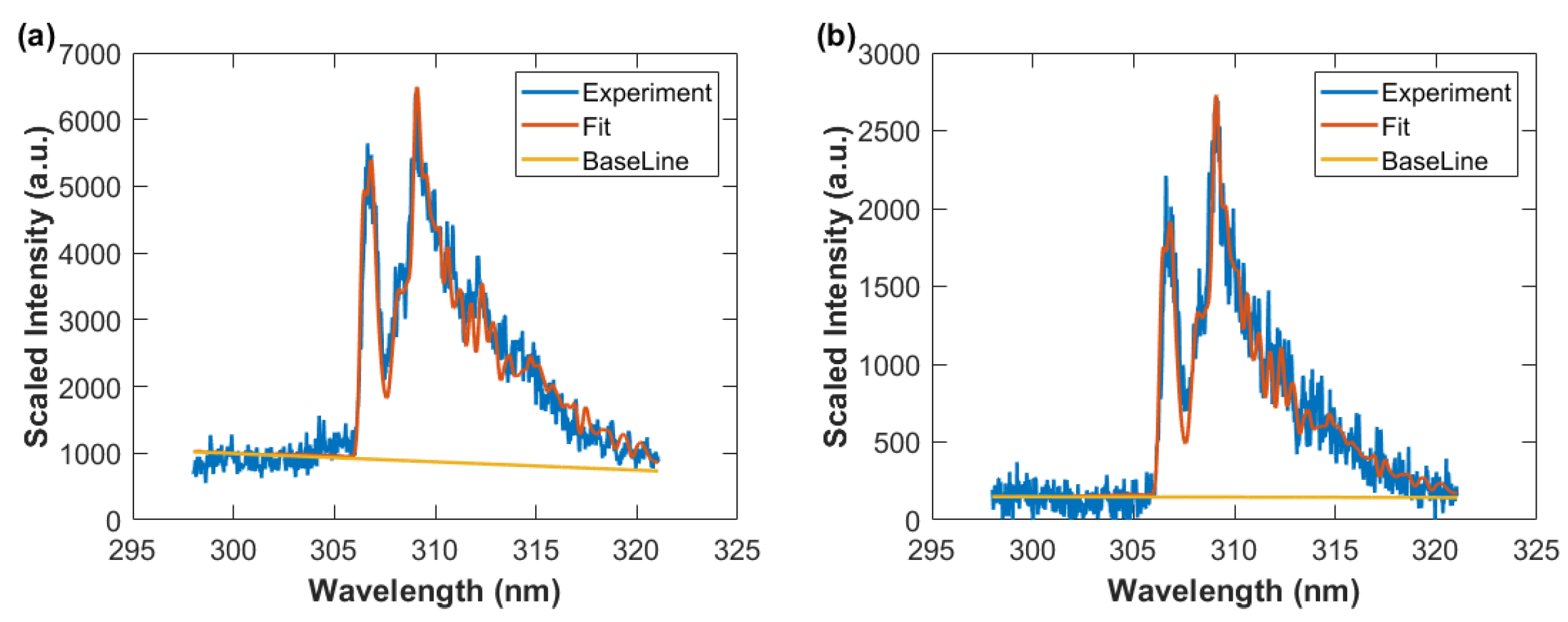
The individual data points in Figure 16 are obtained by fitting the captured data to computed OH spectra. Figure 17 illustrates the results for time delays of 50 μs and 100 μs at the the slit height of 6.43 mm.
In combustion investigation of for example hydrocarbon laser ignition, OH signals are significantly larger than those obtained in laboratory air breakdown. However, planar laser induced fluorescence, or planar LIF, is usually applied in laser-initiated combustion that allows one to correlate shadow graphs with fluid physics expansion of the kernel [14,15]. However, spectra of CN that are recorded within the first μs after initiation of laser plasma in laboratory can be associated with the expanding shock wave [22]. An increase in electron density is inferred near the shockwave from analysis of a carbon atomic line superposed with the CN emission spectrum, and Abel inversion techniques allows one to associate increased CN density near the expanding shock wave.
4. Conclusions
A correlation of spatially- and temporally- resolved OH emission spectra and of shadow graphs is challenging. OH signals are discernible early in the laser-plasma and appear spectrally interference-free at time delays of typically 50 μs after optical air breakdown. For time delays of the order of 50 to 100 μs, fluid physics phenomena become apparent and appear cylindrically symmetric, but the laser-plasma kernel can not be modeled as spherically symmetry. For time delays of 1 μs, the shock wave appears spherically symmetric allowing one to utilize Abel inverse integral techniques for determination of the spatial electron density and diatomic molecular CN distribution. However, when utilizing chemical equilibrium distribution predictions for moisture laden air, one can associate shadow graphs, captured for time delays of typically 50 μs and 100 μs, with corresponding spatiotemporally resolved OH emission. From the fitted OH temperature one can infer OH densities of ∼3 × 1016 cm−3 for 25% relative humidity laboratory air, and slight OH density variations that are associated with optical-breakdown-kernel fluid dynamic expansion for time delays of the order of 100 μs.
Funding
This research received no specific grant-number external funding.
Institutional Review Board Statement
Not applicable.
Informed Consent Statement
Not applicable.
Data Availability Statement
Not applicable.
Acknowledgments
The author acknowledges support in part the State of Tennessee funded Center for Laser Applications at the University of Tennessee Space Institute.
Conflicts of Interest
The author declares no conflict of interest. The funders had no role in the design of the study; in the collection, analyses, or interpretation of data; in the writing of the manuscript, or in the decision to publish the results.
Abbreviations
The following abbreviations are used in this manuscript:
| CN | Cyanide |
| BESP | Boltzmann Equilibrium Spectrum Program |
| ICCD | intensified Charge-Coupled Device |
| LIBS | Laser-Induced Breakdown Spectroscopy |
| Nd:YAG | Neodymium-doped Yttrium Aluminium Garnet |
| NMT | Nelder-Mead Temperature |
| OH | Hydroxyl |
| SATP | Standard Ambient Temperature Pressure |
References
- Kunze, H.-J. Introduction to Plasma Spectroscopy; Springer: Berlin/Heidelberg, Germany, 2009. [Google Scholar]
- Fujimoto, T. Plasma Spectroscopy; Clarendon Press: Oxford, UK, 2004. [Google Scholar]
- Ochkin, V.N. Spectroscopy of Low Temperature Plasma; Wiley-VCH: Weinheim, Germany, 2009. [Google Scholar]
- Boulos, M.I.; Fauchais, P.; Pfender, E. Thermal Plasmas. Fundamentals and Applications; Plenum Press: London, UK, 1994. [Google Scholar]
- Nugroho, S.K.; Kawahara, H.; Gibson, N.P.; de Mooij, E.J.W.; Hirano, T.; Kotani, T.; Kawashima, Y.; Masuda, K.; Brogi, M.; Birkby, J.L.; et al. First Detection of Hydroxyl Radical Emission from an Exoplanet Atmosphere: High-dispersion Characterization of WSAP-33b Using Subaru/IRD. Astrophys. J. Lett. 2021, 910, L9. [Google Scholar] [CrossRef]
- Stützer, R.; Oschwald, M. The Hyperfine Structure of the OH* Emission Spectrum and its Benefits for Combustion Analysis. In Proceedings of the 8th European Conference for Aeronautics and Space Sciences (EUCASS), Madrid, Spain, 1–4 July 2019; p. 2019–839. [Google Scholar]
- Radziemski, L.J.; Cremers, D.A. (Eds.) Laser-Induced Plasmas and Applications; Dekker: New York, NY, USA, 1989. [Google Scholar]
- Miziolek, A.W.; Palleschi, V.; Schechter, I. (Eds.) Laser Induced Breakdown Spectroscopy (LIBS): Fundamentals and Applications; Cambridge University Press: New York, NY, USA, 2006. [Google Scholar]
- Singh, J.P.; Thakur, S.N. (Eds.) Laser-Induced Breakdown Spectroscopy, 2nd ed.; Elsevier: Amsterdam, The Netherlands, 2020. [Google Scholar]
- De Giacomo, A.; Hermann, J. Laser-induced plasma emission: From atomic to molecular spectra. J. Phys. D Appl. Phys. 2017, 50, 183002. [Google Scholar] [CrossRef]
- Parigger, C.G.; Helstern, C.M.; Jordan, B.S.; Surmick, D.M.; Splinter, R. Laser-Plasma Spectroscopy of Hydroxyl with Applications. Molecules 2020, 25, 988. [Google Scholar] [CrossRef] [PubMed] [Green Version]
- Parigger, C.G. Features of Hydroxyl Emission Spectroscopy in Laboratory-Air Laser-Plasma. Int. Rev. At. Mol. Phys. 2022, 13, 15–25. [Google Scholar]
- Fatima, H.; Ullah, M.U.; Ahmad, S.; Imran, M.; Sajjad, S.; Hussain, S.; Qayyum, A. Spectroscopic evaluation of vibrational temperature and electron density in reduced pressure radio frequency nitrogen plasma. SN Appl. Sci. 2021, 3, 646. [Google Scholar] [CrossRef]
- Chen, Y.-L.; Lewis, J.W.L. Visualization of laser-induced breakdown and ignition. Opt. Express 2001, 9, 360–372. [Google Scholar] [CrossRef] [PubMed]
- Qin, W.; Chen, Y.-L.; Lewis, J.W.L. Time-resolved temperature images of laser-ignition using OH two-line laser-induced fluorescence (LIF) thermometry. Int. Flame Res. Found. (IFRF) Combust. J. 2005, 8, 200508. [Google Scholar]
- Parigger, C.G.; Guan, G.; Hornkohl, J.O. Measurement and analysis of OH emission spectra following laser-induced optical breakdown in air. Appl. Opt. 2003, 42, 5986–5991. [Google Scholar] [CrossRef] [PubMed]
- Parigger, C.G. Laser-induced breakdown in gases: Experiments and simulation. In Laser Induced Breakdown Spectroscopy (LIBS): Fundamentals and Applications; Miziolek, A.W., Palleschi, V., Schechter, I., Eds.; Cambridge University Press: New York, NY, USA, 2006; Chapter 4; pp. 171–193. [Google Scholar]
- Parigger, C.G.; Surmick, D.M.; Helstern, C.M.; Gautam, G.; Bol’shakov, A.A.; Russo, R. Molecular Laser-Induced Breakdown Spectroscopy. In Laser Induced Breakdown Spectroscopy, 2nd ed.; Singh, J.P., Thakur, S.N., Eds.; Elsevier: Amsterdam, The Netherlands, 2020; Chapter 7, pp. 167–212. [Google Scholar]
- Parigger, C.G.; Hornkohl, J.O. Quantum Mechanics of the Diatomic Molecule with Applications; IOP Publishing: Bristol, UK, 2020. [Google Scholar]
- Parigger, C.G.; Woods, A.C.; Surmick, D.M.; Gautam, G.; Witte, M.J.; Hornkohl, J.O. Computation of diatomic molecular spectra for selected transitions of aluminum monoxide, cyanide, diatomic carbon, and titanium monoxide. Spectrochim. Acta Part B At. Spectrosc. 2015, 107, 132–138. [Google Scholar] [CrossRef]
- Parigger, C.G. Review of spatiotemporal analysis of laser-induced plsama in gases. Spectrochim. Acta Part B At. Spectrosc. 2021, 179, 106122. [Google Scholar] [CrossRef]
- Parigger, C.G.; Helstern, C.M.; Jordan, B.S.; Surmick, D.M.; Splinter, R. Laser-Plasma Spatiotemporal Cyanide Spectroscopy and Applications. Molecules 2020, 25, 615. [Google Scholar] [CrossRef] [Green Version]
- Gordon, S.; McBride, B. Computer Program for Calculation of Complex Equilibrium Compositions, Rocket Performance, Incident and Reflected Shocks, and Chapman-Jouguet Detonations; NASA Lewis Research Center, Interim Revision, NASA Report SP-273; NASA: Washinton, DC, USA, 1976. [Google Scholar]
- McBride, B.J.; Gordon, S. Computer Program for Calculating and Fitting Thermodynamic Functions; NASA RP-1271; 2005 Version; NASA: Washinton, DC, USA, 1992. Available online: https://cearun.grc.nasa.gov/ (accessed on 14 December 2019).
- Thiyagarajan, M.; Thompson, S. Optical breakdown threshold investigation of 1064 nm laser induced air plasmas. J. Appl. Phys. 2012, 111, 073302. [Google Scholar] [CrossRef]
- Budnik, A.P.; Vakulovskii, A.S. Constant of Optical-Breakdown Avalanche Development in Moist Air; Atmospheric Optics (A91-29962 11-46); Gidrometeoizdat: Moscow, Russia, 1990; pp. 33–37. (In Russian) [Google Scholar]
- Condon, E.U.; Shortley, G. The Theory of Atomic Spectra; Cambridge University Press: Cambridge, UK, 1953. [Google Scholar]
- MATLAB Release R2022a Update 5; The MathWorks, Inc.: Natick, MA, USA, 2022.
- Surmick, D.M.; Hornkohl, J.O.; The University of Tennessee, University of Tennessee Space Institute, Tullahoma, TN, USA. Personal communication, 25 April 2016.
- Deans, S.R. The Radon Transform and Some Of Its Applications; John Wiley: New York, NY, USA, 1983. [Google Scholar]
- Radon, J. On the determination of functions from their integral values along certain manifolds. J. IEEE Trans. Med. Imaging 1986, 5, 170–176. [Google Scholar] [CrossRef] [PubMed]
- Eschlböck-Fuchs, S.; Demidov, A.; Gornushkin, I.B.; Schmid, T.; Rössler, R.; Huber, N.; Panne, U.; Pedarnig, J.D. Tomography of homogenized laaser-induced plasma by Radon transform technique. Spectrochim. Acta Part B At. Spectrosc. 2016, 123, 59–67. [Google Scholar] [CrossRef]
- Hertel, I.V.; Schulz, C.-P. Atoms, Molecules and Optical Physics 1, Atoms and Spectroscopy; Springer: Berlin/Heidelberg, Germany, 2015. [Google Scholar]
Figure 1.
Experimental arrangement for laser-induced breakdown spectroscopy.

Figure 2.
Module for recording shadow graphs of optical breakdown in air. The attenuated Quantel laser beam is focused with f/20 optics. The asterisk symbolically indicates optical breakdown. The interaction area is illuminated by time-delayed Continuum Surelite laser beams, and shadows are projected onto a screen and recorded with a digital camera [11].

Figure 3.
Computed spectra: T = 4000 K; Spectral resolution (a) 0.001 nm and (b) 0.35 nm.

Figure 4.
Measured and fitted OH spectra, T = 3390 K, spectral resolution: 0.35 nm. The blue circles and red line indicate experimental and fitted data, respectively. The straight line shows the fitted base line that represents an assumed, linearly varying background.
Figure 4.
Measured and fitted OH spectra, T = 3390 K, spectral resolution: 0.35 nm. The blue circles and red line indicate experimental and fitted data, respectively. The straight line shows the fitted base line that represents an assumed, linearly varying background.

Figure 5.
Single-shot shadow graph of the expanding laser-induced plasma initiated with a 170-mJ, 6-ns, 1064-nm focused beam, and imaged using a 5-ns, 532-nm back-light that shows intensity variations and is time-delayed by 1.15 μs (a,b). Double exposure images for time delays of 1 μs and 0.1 μs (c,d).

Figure 6.
Single-shot shadow graph of the expanding laser-induced plasma initiated with a 170-mJ, 6-ns, 1064-nm focused beam, and imaged using a 5-ns, 532-nm back-light that shows intensity variations and is time-delayed by 54.25 μs (a–d) display images from separate laser pulses.
Figure 6.
Single-shot shadow graph of the expanding laser-induced plasma initiated with a 170-mJ, 6-ns, 1064-nm focused beam, and imaged using a 5-ns, 532-nm back-light that shows intensity variations and is time-delayed by 54.25 μs (a–d) display images from separate laser pulses.

Figure 7.
Single-shot shadow graph of the expanding laser-induced plasma initiated with a 170-mJ, 6-ns, 1064-nm focused beam, and imaged using a 5-ns, 532-nm back-light that shows intensity variations and is time-delayed by 104.25 μs (a–d) display images from separate laser pulses.
Figure 7.
Single-shot shadow graph of the expanding laser-induced plasma initiated with a 170-mJ, 6-ns, 1064-nm focused beam, and imaged using a 5-ns, 532-nm back-light that shows intensity variations and is time-delayed by 104.25 μs (a–d) display images from separate laser pulses.

Figure 8.
Recorded data of slit-height vs. wavelength. Gate width: 10 μs, time delay (a) 10 μs—primarily N2 second positive spectra, (b) 20 μs, (c) 30 μs, and (d) 40 μs. The A-X 0-0 band edge is identified in figure (b). Each pseudo-colored image is scaled from minimum to maximum with intensity values as indicated next to the color bar.

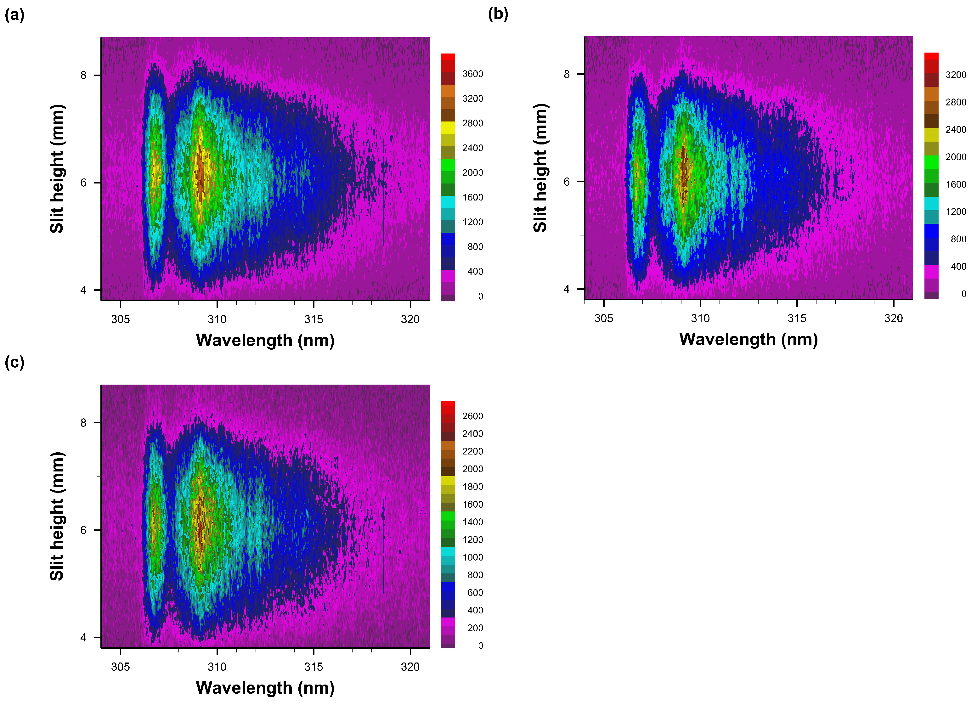
Figure 9.
Recorded data of slit-height vs. wavelength. Gate width: 10 μs, time delay (a) 50 μs—primarily OH spectra, (b) 60 μs, (c) 70 μs, and (d) 80 μs. Each pseudo-colored image is scaled from minimum to maximum with intensity values as indicated next to the color bar.
Figure 9.
Recorded data of slit-height vs. wavelength. Gate width: 10 μs, time delay (a) 50 μs—primarily OH spectra, (b) 60 μs, (c) 70 μs, and (d) 80 μs. Each pseudo-colored image is scaled from minimum to maximum with intensity values as indicated next to the color bar.

Figure 10.
Recorded data of slit-height vs. wavelength. Gate width: 10 μs, time delay (a) 90 μs, (b) 100 μs, and (c) 110 μs. Each pseudo-colored image is scaled from minimum to maximum with intensity values as indicated next to the color bar.
Figure 10.
Recorded data of slit-height vs. wavelength. Gate width: 10 μs, time delay (a) 90 μs, (b) 100 μs, and (c) 110 μs. Each pseudo-colored image is scaled from minimum to maximum with intensity values as indicated next to the color bar.

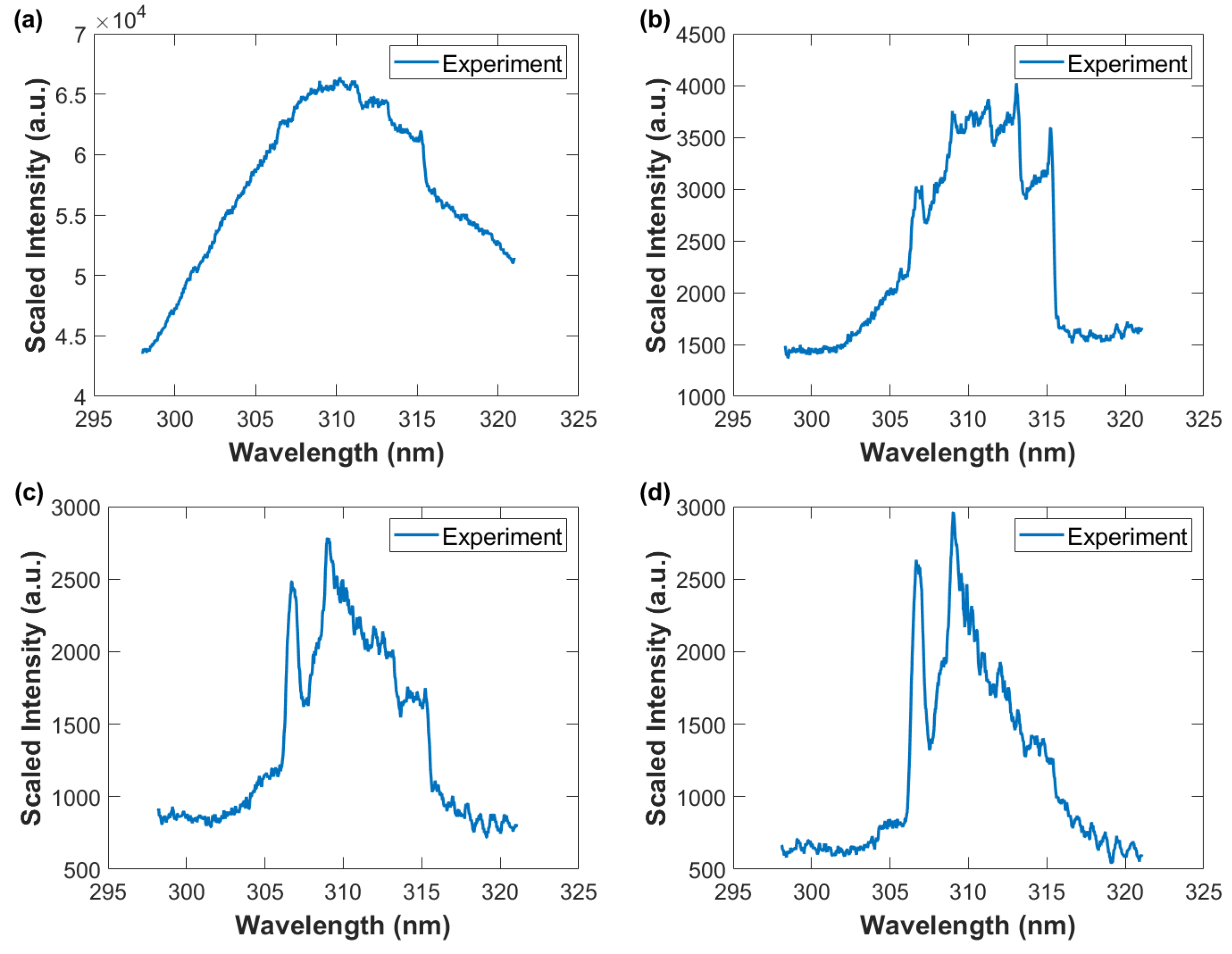
Figure 11.
Wavelength-calibrated and sensitivity-corrected spectra average vs. wavelength. The OH A-X 0-0 band edge near 306 nm is the initial indicator of presence of the hydroxyl radical. Gate width: 10 μs, time delay (a) 10 μs—OH and N2 second positive barely developed (b) 20 μs—primarily N2 second positive spectra, (c) 30 μs, and (d) 40 μs—primarily OH uv A-X spectra.

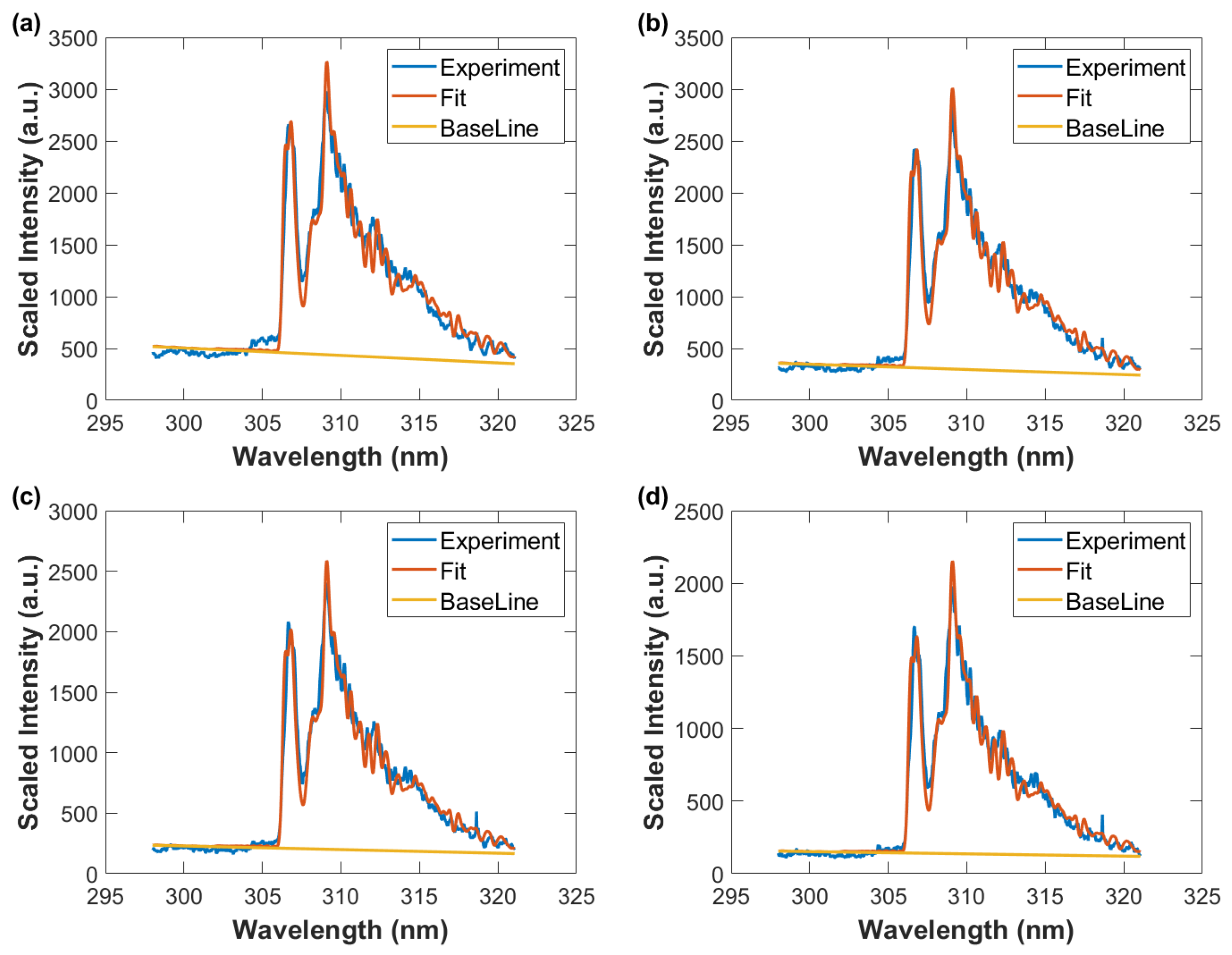
Figure 12.
Wavelength-calibrated and sensitivity-corrected spectra average vs. wavelength, fitted data with spectral resolution of 0.35 nm, and baseline. Gate width: 10 μs, time delay (a) 50 μs, T = 3290 K, (b) 60 μs, T = 3190 K (c) 70 μs, T = 3050 K, and (d) 80 μs, T = 2930 K.
Figure 12.
Wavelength-calibrated and sensitivity-corrected spectra average vs. wavelength, fitted data with spectral resolution of 0.35 nm, and baseline. Gate width: 10 μs, time delay (a) 50 μs, T = 3290 K, (b) 60 μs, T = 3190 K (c) 70 μs, T = 3050 K, and (d) 80 μs, T = 2930 K.

Figure 13.
Wavelength calibrated and sensitivity corrected spectra average vs. wavelength, fitted data with spectral resolution of 0.35 nm, and baseline. Gate width: 10 μs, time delay (a) 90 μs, T = 2780 K (b) 100 μs, T = 2690 K, and (c) 110 μs, T = 2640 K.
Figure 13.
Wavelength calibrated and sensitivity corrected spectra average vs. wavelength, fitted data with spectral resolution of 0.35 nm, and baseline. Gate width: 10 μs, time delay (a) 90 μs, T = 2780 K (b) 100 μs, T = 2690 K, and (c) 110 μs, T = 2640 K.

Figure 14.
Inferred temperature from spatial averages of the displayed images for 10 μs to 110 μs. The dashed line indicates a double exponential fit to the data, see text.
Figure 14.
Inferred temperature from spatial averages of the displayed images for 10 μs to 110 μs. The dashed line indicates a double exponential fit to the data, see text.

Figure 15.
Equilibrium density of OH versus average temperature for a relative humidity of 25 percent. The data points correspond to the indicated time delays. Maximum OH density of 3.17 × 1016 cm−3 occurs at a temperature of 3.144 K. The occurrence of the OH density maximum is a result from equilibrium chemistry calculations as function of temperature.

Figure 16.
Temperature versus slit height for time delays of 50 μs and 100 μs. The horizontal dotted line indicates the temperature of 3144 K at which the OH density maximizes to 3.17 × 1016 cm−3.
Figure 16.
Temperature versus slit height for time delays of 50 μs and 100 μs. The horizontal dotted line indicates the temperature of 3144 K at which the OH density maximizes to 3.17 × 1016 cm−3.

Figure 17.
Spectrum fitting results for slit height of 6.43 mm and spectral resolution of 0.35 nm. (a) T = 3374 K, time delay 50 μs, (b) T = 2580 K, time delay 100 μs.
Figure 17.
Spectrum fitting results for slit height of 6.43 mm and spectral resolution of 0.35 nm. (a) T = 3374 K, time delay 50 μs, (b) T = 2580 K, time delay 100 μs.


Table 1.
Mole fractions for T = 2500 K, T = 3100 K, and T = 3750 K, from computation of air species with the CEA-program, and for 25% relative humidity.
Table 1.
Mole fractions for T = 2500 K, T = 3100 K, and T = 3750 K, from computation of air species with the CEA-program, and for 25% relative humidity.
| Species | Mole Fraction for 2500 K | Mole Fraction for 3100 K | Mole Fraction for 3750 K |
|---|---|---|---|
| e− | 4.147 × 10⁻¹⁰ | 4.916 × 10⁻⁸ | 1.3111 × 10⁻⁶ |
| Ar | 9.1983 × 10⁻³ | 8.9044 × 10⁻³ | 8.1562 × 10⁻³ |
| H | 2.7114 × 10⁻⁴ | 4.4885 × 10⁻³ | 1.3839 × 10⁻² |
| H+ | - | - | 1.585 × 10⁻¹² |
| H− | - | - | 1.653 × 10⁻¹⁰ |
| HNO | 9.4651 × 10⁻⁸ | 4.3791 × 10⁻⁷ | 3.7013 × 10⁻⁷ |
| HNO2 | 8.4537 × 10⁻⁸ | 6.3610 × 10⁻⁸ | 9.598 × 10⁻⁹ |
| HO2 | 4.0794 × 10⁻⁶ | 6.6671 × 10⁻⁶ | 1.8016 × 10⁻⁶ |
| H2 | 1.1744 × 10⁻⁴ | 4.5033 × 10⁻⁴ | 1.9256 × 10⁻⁴ |
| H2O | 8.7192 × 10⁻³ | 2.8062 × 10⁻³ | 1.3692 × 10⁻⁴ |
| H2O2 | 2.7318 × 10⁻⁸ | 2.1904 × 10⁻⁸ | 1.424 × 10⁻⁹ |
| N | 2.524 × 10⁻⁷ | 2.192 × 10⁻⁵ | 5.4050 × 10⁻⁴ |
| N+ | - | - | 1.489 × 10⁻¹⁴ |
| N− | - | - | 2.236 × 10⁻¹² |
| NH | 3.634 × 10⁻⁹ | 1.943 × 10⁻⁷ | 1.3517 × 10⁻⁶ |
| NH2 | 1.103 × 10⁻¹⁰ | 2.329 × 10⁻⁹ | 3.358 × 10⁻⁹ |
| NO | 2.1548 × 10⁻² | 4.3043 × 10⁻² | 4.6896 × 10⁻² |
| NO+ | 4.410 × 10⁻¹⁰ | 5.107 × 10⁻⁸ | 1.3420 × 10⁻⁶ |
| NO2 | 1.8594 × 10⁻⁵ | 1.9773 × 10⁻⁵ | 9.4889 × 10⁻⁶ |
| N2 | 7.5738 × 10⁻¹ | 7.2208 × 10⁻¹ | 6.5741 × 10⁻¹ |
| N2− | - | - | 7.627 × 10⁻¹³ |
| N2+ | - | - | 5.901 × 10⁻¹¹ |
| N2O | 1.1849 × 10⁻⁶ | 2.3699 × 10⁻⁶ | 2.5855 × 10⁻⁶ |
| N3 | - | - | 2.874 × 10⁻¹⁰ |
| O | 6.3014 × 10⁻³ | 6.0120 × 10⁻² | 2.1044 × 10⁻¹ |
| O+ | - | - | 2.075 × 10⁻¹¹ |
| O− | 7.548 × 10⁻¹² | 1.339 × 10⁻⁹ | 3.0021 × 10⁻⁸ |
| OH | 4.5941 × 10⁻³ | 1.0814 × 10⁻² | 5.4876 × 10⁻³ |
| O2 | 1.918 × 10⁻¹ | 1.4724 × 10⁻¹ | 5.6886 × 10⁻² |
| O2+ | - | - | 1.346 × 10⁻⁹ |
| O2− | - | - | 1.124 × 10⁻⁹ |
| O3 | 3.0933 × 10⁻⁸ | 9.5514 × 10⁻⁸ | 7.9000 × 10⁻⁸ |
Publisher’s Note: MDPI stays neutral with regard to jurisdictional claims in published maps and institutional affiliations. |
© 2022 by the author. Licensee MDPI, Basel, Switzerland. This article is an open access article distributed under the terms and conditions of the Creative Commons Attribution (CC BY) license (https://creativecommons.org/licenses/by/4.0/).
Share and Cite
MDPI and ACS Style
Parigger, C.G. Hydroxyl Spectroscopy of Laboratory Air Laser-Ignition. Foundations 2022, 2, 934-948. https://doi.org/10.3390/foundations2040064
AMA Style
Parigger CG. Hydroxyl Spectroscopy of Laboratory Air Laser-Ignition. Foundations. 2022; 2(4):934-948. https://doi.org/10.3390/foundations2040064
Chicago/Turabian StyleParigger, Christian G. 2022. "Hydroxyl Spectroscopy of Laboratory Air Laser-Ignition" Foundations 2, no. 4: 934-948. https://doi.org/10.3390/foundations2040064