Article

Conditions for Scalar and Electromagnetic Wave Pulses to Be “Strange” or Not

by
Peeter Saari
1,2,* and
Ioannis M. Besieris
3
1
Institute of Physics, University of Tartu, W. Ostwaldi 1, 50411 Tartu, Estonia
2
Estonian Academy of Sciences, Kohtu 6, 10130 Tallinn, Estonia
3
The Bradley Department of Electrical and Computer Engineering, Virginia Polytechnic Institute and State University, Blacksburg, VA 24060, USA
*
Author to whom correspondence should be addressed.
Foundations 2022, 2(1), 199-208; https://doi.org/10.3390/foundations2010012
Submission received: 26 December 2021 / Revised: 30 January 2022 / Accepted: 4 February 2022 / Published: 7 February 2022
(This article belongs to the Special Issue Advances in Fundamental Physics)

Abstract

:
Vector-valued electromagnetic waves for which the integral of the electric field over time is zero at every location in space were characterized as “usual” by Bessonov several decades ago. Otherwise, they were called “strange”. Recently, Popov and Vinogradov studied conditions leading to usual waves using a spectral representation. Their main result is that pulses of finite energy in free space are usual and, consequently, bipolar. However, they do not exclude the possibility of the existence of finite-energy strange pulses, although quite exotic, in a vacuum. Our emphasis in this article is to examine what the relevant necessary and sufficient conditions are for usual and strange waves, particularly for scalar pulses. Illustrative examples are provided, including spherical symmetric collapsing pulses, propagation-invariant, and the so-called almost undistorted spatiotemporally localized waves. Finally, source-generated strange electromagnetic fields are reported.

1. Introduction

Progress in the generation and application of femtosecond and attosecond electromagnetic (EM) pulses have stimulated theoretical research of few-cycle and near-cycle localized exact solutions of the free-space wave equation (see, e.g., [1,2] and references therein). A strong space-time coupling, inherent to such pulses in focusing, makes the classical well-known approximations inapplicable. Moreover, with the decrease in the duration of optical pulses, there is a growing need to go beyond the quasi-monochromatic limit, and spectral representations of fields lose their advantages over direct time-domain ones. There is an ultimate milestone on the road away from the narrow-band limit—where the temporal spectrum of the pulse extends to the frequency scale origin. This causes a merging of positive-frequency and negative-frequency Fourier components, and as a result, the concept of analytic signal with its Hilbert-transform-related real and imaginary parts remains the only sound alternative for determining the envelope of a pulse.
If the spectrum vanishes at the frequency ω = 0 , the pulse is bipolar. Several decades ago Bessonov [3] introduced the term “strange” for waves whose electric field does not obey the equality
S E ( r ) E ( r , t ) d t = 0
and called “usual” all waves satisfying Equation (1) at every location r . It is obvious that usual waves are necessarily bipolar.
In a recent paper [4], Popov and Vinogradov studied conditions leading to Equation (1) using a spectral representation. Their main result is that pulses of finite energy in free space are usual and, consequently, bipolar. However, they do not exclude the possibility of the existence of finite-energy strange pulses, although quite exotic, in a vacuum. In other words, they have not proved that the finiteness of pulse energy is a sufficient condition for a pulse to be usual (not strange). Of course, it is not a necessary condition, as a bipolar plane wave pulse can already readily be a usual one.
We will neither question the results of the paper [4] nor prove the sufficiency of the energy condition. Instead, our aims here are to analyze what the relevant necessary and sufficient conditions are and to study the problem with several sample waves.
Specifically, we first consider spherically symmetric pulses converging to and thereafter, at positive times, diverging from a focus at the origin, i.e., pulses described by a wavefunction
ψ ( r , t ) = 1 r [ f ( t + r / c ) f ( t r / c ) ] ,
where f ( s ) is an arbitrary nonsingular function depending on the spherical radial coordinate r = x 2 + y 2 + z 2 and time t , with c being the speed of light in a vacuum.
Second, we consider axially symmetric propagation-invariant pulses [5,6,7,8,9,10] whose wavefunction and/or energy density depend on the axial coordinate and time solely through the propagation variable ζ = z v t , where v is the group velocity of the pulse. These fields exhibit pronounced space-time coupling. From a theoretical point of view it is interesting that the second type of pulses can be obtained from spherically symmetric ones via relativistic boosts and/or complexifying the axis z [5,6,8]. Finally, we study some exotic pulses described by sophisticated solutions of the wave equation.

2. Methods

We primarily analyze scalar waves for the following reasons:
  • Every component of the electric (and magnetic) field is a scalar-valued field that obeys the wave equation. Hence, in order to judge for a chosen wavefunction ψ ( r , t ) whether the corresponding EM pulse is strange or not, it is sufficient to evaluate the integral
    S ψ ( r ) = ψ ( r , t ) d t .
  • If EM field vectors are derived by the standard procedure of constructing the magnetic vector potential or the Hertz vector from ψ ( r , t ) , even simple expressions of ψ ( r , t ) may result in too cumbersome ones for the EM field vectors, and the integral of Equation (1) may be difficult to evaluate. Moreover, as the procedure involves taking derivatives with respect to time and/or spatial coordinates, a strange ψ ( r , t ) , i.e., one with property S ψ ( r ) 0 , generally results in a usual EM field, i.e., S E ( r ) = 0 .
  • The notion of strangeness also applies to wave fields that are scalar valued by their physical nature, e.g., sound waves.
It should be pointed out that our approach does not mean resorting to a scalar approximation for EM fields.
In order to determine whether an electric field is strange or not, one can avoid integration according to Equation (1), which in most cases is a computationally difficult task. Instead, one can make use of the expression E ( r , t ) = A ( r , t ) / t   of the electric field derived from a magnetic vector potential in the Coulomb gauge and consider the vector potential at t = ± instead of evaluation the integral of the electric field. It is convenient to derive the vector potential from a scalar wavefunction as A ( r , t ) = × [ ψ ( r , t ) a z ] , where a z is the unit vector along the z -axis. In the case of cylindrical symmetry, only the azimuthal component remains, and it takes the simple form A φ ( ρ , z , t ) = ψ ( ρ , z , t ) / ρ . In the case of spherical symmetry, the unit vector a z needs to first be expressed in a spherical coordinate system, and then for the curl, only the azimuthal component remains, taking a similar simple form A φ ( r , θ , t ) = sin θ ψ ( r , θ , t ) / r . Hence, if one of the following equalities is fulfilled at every location, in the case of cylindrical or spherical symmetry, respectively,
lim t ρ [ ψ ( ρ , z , t ) ψ ( ρ , z , t ) ] = 0 , lim t r [ ψ ( r , θ , t ) ψ ( r , θ , t ) ] sin θ = 0 ,
the corresponding electric field is not strange. Equation (4) has been successfully applied for the examples in Section 3.

2.1. Evaluation of the Wave Pulse Energy

The (total) energy of a physically realizable pulse is a time-independent spatial integral (over the whole space) of the energy density, which in the case of an EM wave is given by the well-known expression with squares of strengths of electric and magnetic fields. Energy density of a scalar field is frequently defined as the square of the wavefunction (or modulus squared for complex-valued fields). However, the spatial integral of the latter will not be used below for establishing whether the EM pulse corresponding to a given wavefunction has finite or infinite energy.
For scalar-valued wave fields, another definition of the energy density exists [11], which is consistent with the energy conservation law and the Poynting theorem. It is given by Equation (5) below. We will call the spatial integral of W the Mandel-Wolf total energy for brevity. Conditions in the spectral domain—analogous to those in [4]—for a scalar field to have finite energy and be usual are discussed in Appendix A.
W = 1 2 [ 1 c 2 ( t ψ ) 2 + ψ · ψ ] .
In order to establish whether a chosen wavefunction gives a pulse of finite energy or not, we used two different packages of scientific calculation for symbolic integration—or, if it turned out to be impossible—numerical integration.

2.2. Time-Domain Representation

As an alternative to using the Fourier expansion of the field as done in [4], for the constituents of the field one may take the singular propagator D ( r , t ) (sometimes called the Riemann or Schwinger function)
D ( r , t ) = 1 4 π r c 2 [ δ ( r / c t ) δ ( r / c + t ) ] G + ( r , t ) G ( r , t ) ,
where δ ( . ) denotes the Dirac delta and G ± are the causal (retarded) and anticausal (advanced) Green functions, respectively. The function D ( r , t ) represents a spherically symmetric delta-shaped pulse wave, first (at negative times t ) collapsing to the origin (the right term) and then (at positive times t ) expanding from it.
With this propagator as an elementary constituent, any solution to the three-dimensional homogeneous wave equation can be expressed as the following convolution integral over the whole 3D space:
ψ ( r , t ) =   [ D ( R , t ) h ( r ) + t D ( R , t ) g ( r ) ] d r .
Here, R = | r r | and the distributions g ( . ) and h ( . ) are determined by the initial conditions—the field “snapshot” at the time origin moment g ( r ) = ψ ( r , 0 ) and h ( r ) = / t   ψ ( r , t ) | t = 0 . However, unlike the solution of a radiation problem, since D contains not only the retarded Green function but the advanced one as well, g and h describe a distribution of fictitious Huygens-type sources, i.e., sources coupled with sinks of the same strength.

3. Results

3.1. General Conditions for a Pulse to Be “Usual”

3.1.1. Sufficient Conditions

With the help of Equation (7), we can easily find conditions under which the field is not “strange”, i.e., conditions of vanishing of the time integral in Equation (3), or—keeping in view the text before it—also conditions for fulfillment of Equation (1). Since D ( R , t ) is an odd function with respect to time, the first term of the integrand in Equation (7) in any case does not contribute to S ψ ( r ) . As the δ -function equals zero at infinity, the time integral of the second term vanishes if R = | r r | remains finite in the spatial integration. Hence, any wave field that is spatially bounded at a certain instant of time (when the pulse is focused) cannot be “strange”. Any such pulse, if it has no unphysical singularities, has finite energy irrespective of which of the abovementioned definitions of the pulse energy has been taken. Hence, the sufficient condition formulated here is consistent with the one found by Popov and Vinogradov [4]. The second term also vanishes if g ( r ) = ψ ( r , 0 ) = 0 in the whole space. This condition means that any nontrivial ψ ( r , t ) must be an odd function of time. Therefore, such oddness is another sufficient condition for a pulse to be “usual”. The results of the next subsection demonstrate accordance with this condition.

3.1.2. Necessary and Sufficient Conditions

For a field to be usual (not strange), the integral in Equation (1) or (3) must vanish everywhere. Therefore, we obtain the necessary condition that it must vanish at the origin r = 0 . In this case, we write R = | r | r , omitting the prime for simplicity. After integration from t = T to t = T and subsequently taking the limit T in accordance with Equation (3), the second term in Equation (7) can be transformed in spherical coordinates as follows:
[ D ( R , t ) g ( r , θ , φ ) R 2 sin θ d R d θ d φ ] T T = = 1 4 π c 2 { r 1 [ δ ( r / c T ) δ ( r / c + T ) δ ( r / c + T ) + δ ( r / c T ) ] g ( r , θ , φ ) r 2 sin θ d r d θ d φ } = = 2 1 4 π g ( c T , θ , φ ) T sin θ d θ d φ = 2 T g c T .
Here, g c T denotes the average value of the function g on the surface of a sphere with radius c T and center at the origin. Therefore, a necessary condition for a wave field to be usual is lim T T g c T = 0 .
Generally, this means that g ( r , θ , φ ) must asymptotically vanish as r faster than 1 / r . Of course, the surface average might be zero irrespective to such asymptotic behavior of g ( r , θ , φ ) if the latter is bipolar on the surface, and due to some symmetry the regions of opposite sign cancel each other. However, if applying the condition for a sphere whose center is shifted from the origin, the symmetry would disappear and the condition would be fulfilled due to only the aforementioned asymptotic behavior of g ( r , θ , φ ) .
The transformation of the integral carried out above remains valid for an arbitrary point r 0 in Equation (7). The reason for this is that whatever the point in the field is, its radial vector is fixed while | r | runs together with c T to infinity. Therefore, r can be neglected in the expression R = | r r | . Consequently, the necessary and sufficient condition for a wavefield to be “usual” can be stated as follows. The wavefunction g ( r , θ , φ ) at t = 0 must vanish asymptotically as r faster than 1 / r ; in other words, the following equality must be fulfilled:
lim r r ψ ( r , θ , φ , 0 ) = 0 .
Application of the criterion in Equation (8) is especially appropriate when ψ ( r , t ) contains multivalued complex functions and direct temporal integration according to Equation (3) may be hampered due to crossing the branch-cut lines.

3.2. Spherically Symmetric Pulses: Some Examples

Such pulses, the general form of the wavefunction of which is given by Equation (2), are the simplest to analyze. If ψ ( r , t ) in the form of Equation (2) is used to construct a vector magnetic potential, simple relations between f ( s ) and EM field vectors and EM pulse energy have been derived in [12] and references therein.

3.2.1. Even and Odd Lorentzians
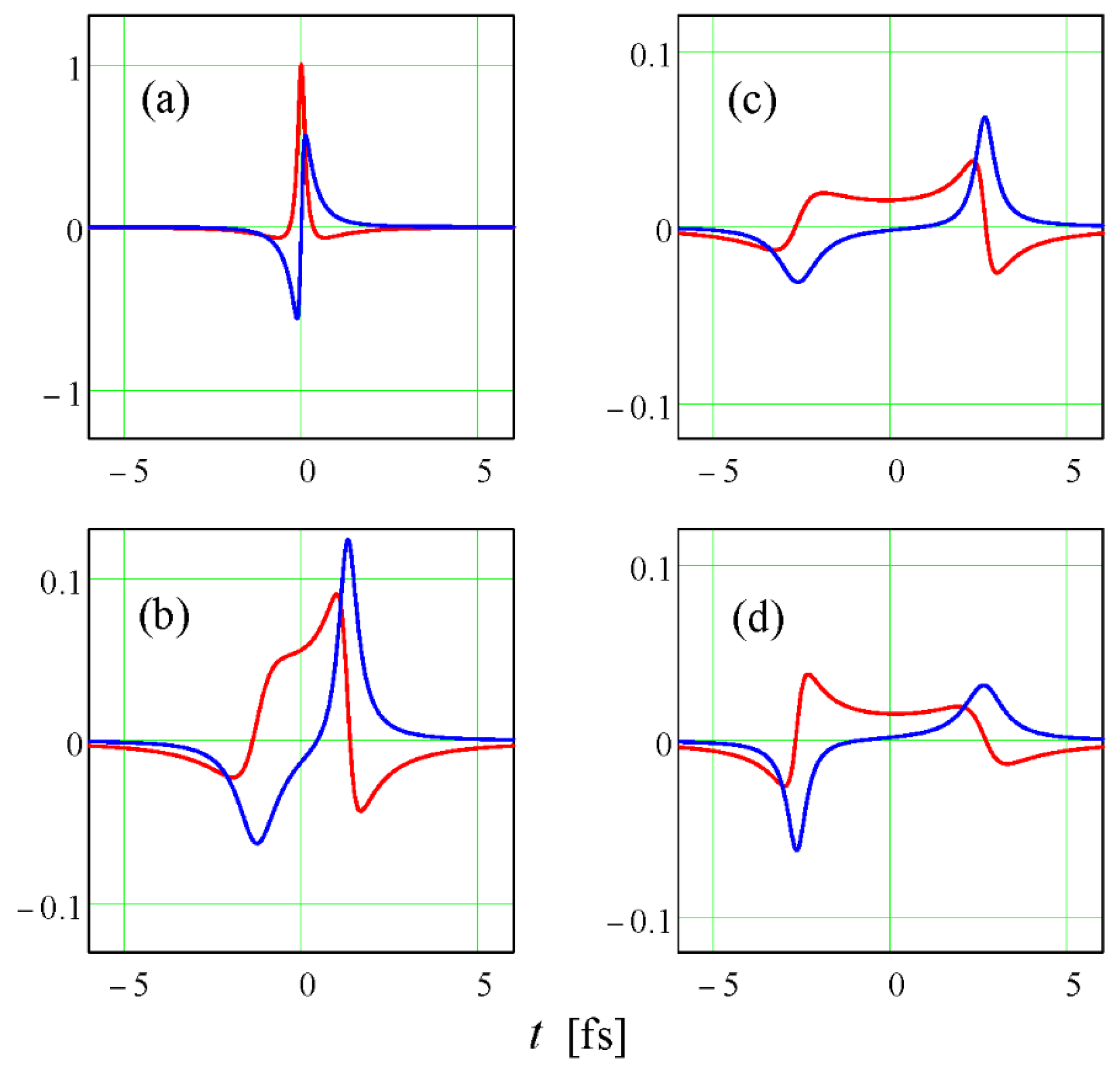
We studied the functions f e ( s ) = 1 / ( 1 + s 2 n ) and f o ( s ) = s / ( 1 + s 2 n ) (see Equation (2)) where n = 1 , 2 , . Results concerning the strangeness of such fields are as follows:
(a)
If f ( s ) is an even function, ψ ( r , t ) is odd with respect to time (hence, automatically not strange) and E ( r , t ) is even, but nevertheless not strange. The magnetic field is odd and, hence, not strange.
(b)
If f ( s ) is odd, ψ ( r , t ) is even with respect to time (but nevertheless not strange) and E ( r , t ) is odd, i.e., automatically is not strange. The magnetic field is even, but still not strange.
For these pulses the Mandel–Wolf energy and EM energy are both finite.

3.2.2. Error Function

The function f ( s ) = erf ( s ) is odd, and consequently, ψ ( r , t ) is even. However, it is strange and it is not square-integrable. Nevertheless, its Mandel–Wolf energy and EM energy are both finite. In accordance with point (b) above, E ( r , t ) is odd, i.e., automatically not strange. The magnetic field is an even function of time but still not strange.

3.3. Propagation-Invariant Pulses: Some Examples

3.3.1. Superluminal X-Waves

Inspired by the quotation “Therefore, the possibility of the existence of strange and unipolar pulses in a vacuum, although quite exotic, remains” from [4], we turned to the so-called X-waves, which were first intruduced in [5,13] and then studied in numerous papers; see [6,7,8,9] and references therein.
The so-called fundamental axisymmetric X-wave is given by
ψ ( ρ , z , t ) = a [ a + i ( z v t ) ] 2 + ρ 2 γ 2   ,
where γ = ( v 2 / c 2 1 ) 1 / 2 is the superluminal version of the Lorentz factor, including the velocity v > c of the pulse; a is a positive parameter that determines the width of the pulse; and ρ = x 2 + y 2 . This wavefunction is commonly considered as a white-spectrum superposition of Bessel beams.
Referring to Equation (7), it can be also derived as Liénard–Wiechert potentials for Lorentzian distributions of fictitous “charges” (sources and sinks) flying with the constant velocity v along the axis z , i.e., the distributions being a [ ( z v t ) 2 + a 2 ] 1 δ ( x ) δ ( y ) (for the imaginary part of ψ ( . ) and ( z v t ) [ ( z v t ) 2 + a 2 ] 1 δ ( x ) δ ( y ) (for the real part) [14]. The real part of Equation (9) respresents a strange scalar field and the imaginary part an ordinary (usual) scalar field. At the origin, ψ ( 0 , 0 , t ) = a / ( a i v t ) , the temporal spectrum of the real part is proportional to exp ( a | ω | / v ) while that of the imaginary part is proportional to signum ( ω ) exp ( a | ω | / v ) . Hence, although both spectra have their maxima at infinitesimally small frequencies, the spectrum of the imaginary part lacks the constituent at ω = 0 exactly, which is in accordance with the established difference in strangeness of the real and imaginary parts.
If the EM vector fields are derived from Equation (9) by standard procedures involving the vector magnetic potential or the Hertz vector, then, due to taking derivatives in the course of these procedures, the EM field turns out to be usual.
A specific procedure to obtain an EM field avoiding the derivatives is to derive the following complex-valued Riemann–Silberstein vector
F ( r , t ) = i c 2 ( v / c ) 2 1 v 2 Q ( r , t ) P ( r , t ) P + ( r , t ) a x c ( v / c ) 2 1 v Q ( r , t ) P ( r , t ) P + ( r , t ) a x + c 2 ( v / c ) 2 1 v 2 Q ( r , t ) a z ; Q ( r , t ) = ( ( v / c ) 2 1 ) ρ 2 + ( a + i ( z v t ) ) 2 ; P ± ( r , t ) = 1 ± a + i ( z v t ) Q ( r , t )
which arises from a superposition of vector-valued Bessel beams. It can be expressed as F ( r , t ) = ε 0 / 2 ( E + i c B ) , where ε 0 is the permittivity of free space and E and B are real fields obeying the homogeneous Maxwell equations. The z -component of F ( r , t ) is essentially the infinite-energy superluminal fundamental X wave, as one can see by inspection of Equations (9) and (10). Hence, the real part of the electric field is a strange field, whereas the magnetic field is a usual field. The EM wave pulse energy is infinite quite analogously to the case of plane waves. This is understandable because the X wave can be thought of as a superposition of plane wave pulses directed along a conical surface.

3.3.2. Subluminal Arctan-Wave

The expression in Reference [6]
ψ ( r , t ) = 1 ρ 2 + γ 2 ( z v t ) 2 tan 1 ( ρ 2 + γ 2 ( z v t ) 2 a + i γ ( v / c ) ( z c 2 v t ) ) ;   γ = 1 / 1 ( v / c ) 2 ,   v < c ,
where again ρ is the polar radial coordinate, is a subluminal localized wave that is relatively undistorted upon propagation depending on the value of the positive free parameter a . The real part of ψ ( r , t ) has a finite Mandel–Wolf total energy and is a strange field; however, its imaginary part is normal (usual). Additionally, the finite-energy corresponding electromagnetic fields, constructed within the framework of either a Coulomb gauge or a vector Hertz potential, are usual fields.

3.3.3. Luminal Localized Wave

In cylindrical coordinates, the azimuthally symmetric expression
ψ ( r , t ) = 1 4 b 2 ρ 2 + [ b 2 + ( a 1 + i ς ) ( a 2 i η ) + ρ 2 ] 2 ,
where ζ = z c t , η = z + c t are the characteristic variables of the one-dimensional scalar wave equation in vacuum and a 1 , 2 and b are positive free parameters, is a spatiotemporally localized extended splash-mode nonsingular solution to the (3 + 1)-dimensional scalar wave equation under the condition a 1 a 2 b 2 > 0 . It can be derived from a superposition of Bessel–Gauss focus wave modes (FWM). For b = 0 , it reduces to the ordinary first-order splash-mode first derived by Ziolkowski (see, e.g., [5,6]); the latter is not strange. The scalar wave field in Equation (12) is not strange, and the Wolf–Mandel total energy of its real part is finite. The electric and magnetic fields arising from a vector potential A ( r , t ) = × [ ψ ( r , t ) a z ] within the framework of a Coulomb gauge have been examined. The electric and magnetic fields are usual. The total electromagnetic energy is finite.
The reason why the “strangeness” integral of Equation (3) turns out to be zero can be understood from Figure 1.
At first glance, the real part is unipolar (à la that of the X wave); i.e., the real field seems to be strange. However, closer inspection of Figure 1a indicates that the peak appears on the negative-polarity background, which makes the area under the curve equal to zero, as is the case with the imaginary part. Plots (a) and (b) show that outside the origin, the pulse splits into two counterpropagating ones. Comparison of plots (c) and (d) shows that the real part of the wavefunction is even with respect to simultaneous inversion of the sign of the variables z ,   t and the imaginary part is odd with respect to the same inversion. It should be mentioned that neither numerical computation of the “strangeness” integral Equation (3) nor plotting of the wavefunction can be properly accomplished by straightforward application of Equation (12) due to presence of a brach cut in the square root function of a complex-valued argument.

3.4. Strange Fields Generated by Sources

3.4.1. Bonnor Fields

In cylindrical coordinates, we identify two regions of space: ρ a (outside) and ρ a (inside). Motivated by Bonnor’s work [15], we specify scalar and vector potentials in the two regions:
Φ 0 ( ρ , ϕ , z , t ) = e ( t z ) 2 cos ϕ / ρ ,   A 0 ( ρ , ϕ , z , t ) = Φ 0 ( ρ , ϕ , z , t ) a z ; Φ i ( ρ , ϕ , z , t ) = e ( t z ) 2 ( 4 ρ 2 a 3 3 ρ 3 a 4 ) cos ϕ ,   A i ( ρ , ϕ , z , t ) = Φ i ( ρ , ϕ , z , t ) a z .
Here, normalization with the speed of light in a vacuum equal to unity has been used. These potential fields satisfy the Lorentz condition. Additionally, the continuity Φ 0 ( a , ϕ , z , t ) = Φ i ( a , ϕ , z , t ) should be noted.
In the region ρ a , the electric volume charge and current densities are determined as follows:
ρ v i = ( 2 2 t 2 ) Φ i = 12 e ( t z ) 2 ( a 2 ρ ) cos ϕ a 4 , J v i = ( 2 2 t 2 ) A i = ρ v i a z .
The total charge in this region equals zero. No charges exist for ρ a .
The electric and magnetic fields in the two regions are given by the expressions
E 0 = Φ 0 A 0 / t = e ( t z ) 2 cos ϕ ρ 2 a ρ + e ( t z ) 2 sin ϕ ρ 2 a ϕ ; B 0 = × A 0 = e ( t z ) 2 sin ϕ ρ 2 a ρ + e ( t z ) 2 cos ϕ ρ 2 a ϕ ; E i = e ( t z ) 2 ρ ( 8 a + 9 ρ ) cos ϕ a 4 a ρ + e ( t z ) 2 ρ ( 4 a 3 ρ ) sin ϕ a 4 a ϕ ; B i = e ( t z ) 2 ρ ( 4 a 3 ρ ) sin ϕ a 4 a ρ e ( t z ) 2 ρ ( 8 a 9 ρ ) cos ϕ a 4 a ϕ ;
These are transverse electromagnetic (TEM) structures propagating along the z -direction with the normalized speed of light in vacuum. Both the electric and magnetic fields are strange. The total energy associated with these fields is finite.

3.4.2. Single-Cycle Dipole Electromagnetic Fields

Wang et al. [16] have derived single-cylce electromagnetic fields generated by an oscillating elecric dipole oriented along the x -direction. We examined these fields for “strangeness”. The electric field is strange but not the magnetic field.

4. Conclusions

Motivated by the recent work of Popov and Vinogradov [4], we have examined the relevant conditions for usual and strange waves, particularly for scalar pulses. General necessary and sufficient conditions for scalar and electromagnetic field pulses possessing spatiotemporal coupling to be “usual” or “strange” have been derived in the time domain, and their application has been illustrated. For various examples of luminal and rather peculiar subluminal and superluminal scalar waves, it has been shown that even if they are strange, the corresponding finite-energy electromagnetic fields constructed from the scalar fields from either a magnetic potential within the framework of a Coulomb gauge or a vector Hertz potential are usual. Finally, source-generated strange electromagnetic fields have been reported.

Author Contributions

Investigation, P.S. and I.M.B.; writing—original draft preparation, P.S. and I.M.B.; writing—review and editing, P.S. and I.M.B. All authors have read and agreed to the published version of the manuscript.

Funding

This research received no external funding.

Institutional Review Board Statement

Not applicable.

Informed Consent Statement

Not applicable.

Data Availability Statement

Not applicable.

Conflicts of Interest

The authors declare no conflict of interest.

Appendix A

Let ψ ( r , t ) be a real function satisfying the homogeneous scalar wave equation in free space. The energy transport equation for such a wavefunction is given by
S + t W = 0 ,
where
W = 1 2 [ 1 c 2 ( t ψ ) 2 + ψ ψ ] ,   S = t ψ   ψ
are, respectively, the real energy density in units J / m 3 and the real energy flow vector ( W / m 2 ).
Let the real field ψ ( r , t ) be expressed in terms of its spatial Fourier spectrum as follows:
ψ ( r , t ) = 1 ( 2 π ) 3 d k Ψ ( k , t ) e i k r .
Then, the total energy density can be written as follows:
W t o t a l = d r   W ( r , t ) = 1 2 1 ( 2 π ) 3 d k [ 1 c 2 Ψ ˙ ( k , t ) Ψ ˙ ( k , t ) + k 2 Ψ ( k , t ) Ψ ( k , t ) ] ,
where the dot indicates differentiation with respect of time. Bearing in mind the dispersion relationship k 2 + ω 2 / c 2 = 0 , we assume, next, the form
Ψ ( k , t ) = Ψ ( k ) e i k c t + Ψ + ( k ) e i k c t .
Then, we have
W t o t a l = 1 2 1 ( 2 π ) 3 d k k 2 [ | Ψ ( k ) | 2 + | Ψ + ( k ) | 2 ] .
Next, let the wavefunction ψ ( r , t ) be defined as ψ ( r , t ) = ϕ ( r , t ) / t and consider the integral
S ψ ( r ) = ψ ( r , t )   d t = L i m | T T T ψ ( r , t )   d t = L i m | T [ ϕ ( r , T ) ϕ ( r , T ) ]
The wavefunction ϕ ( r , T ) is expressed as
ϕ ( r , T ) = d k e i k r [ Φ ( k ) e i k c T + Φ + ( k ) e i k c T ] .
According to the Riemann–Lebesgue theorem, S ψ ( r ) vanishes provided that
0 d k   k 2 | d Ω   Φ ± ( k ) e i k r |
converges. However, Φ ± ( k ) = Φ ± ( k ) / c k . Therefore, S ψ ( r ) vanishes and the field is usual provided that the integral
0 d k   k | d Ω   Ψ ± ( k ) e i k r |
converges.

References

  1. Lekner, J. Theory of Electromagnetic Pulses; Morgan & Claypool Publishers: San Rafael, CA, USA, 2018. [Google Scholar]
  2. Kiselev, A.P. Localized Light Waves: Paraxial and Exact Solutions of the Wave Equation (a Review). Opt. Spectrosc. 2007, 102, 603–622. [Google Scholar] [CrossRef]
  3. Bessonov, E.G. On a class of electromagnetic waves. Zh. Eksp. Teor. Fiz. 1981, 80, 852–858. [Google Scholar]
  4. Popov, N.L.; Vinogradov, A.V. Free Space Strange and Unipolar EM Pulses: Yes or No? Foundations 2021, 1, 169–174. [Google Scholar] [CrossRef]
  5. Ziolkowski, R.W.; Besieris, I.M.; Shaarawi, A.M. Aperture realizations of exact solutions to homogeneous-wave equations. Opt. Soc. Am. A 1993, 10, 75–87. [Google Scholar] [CrossRef]
  6. Besieris, I.; Abdel-Rahman, M.; Shaarawi, A.; Chatzipetros, A. Two fundamental representations of localized pulse solutions to the scalar wave equation. Prog. Electromagn. Res. 1998, 19, 1–47. [Google Scholar] [CrossRef] [Green Version]
  7. Salo, J.; Fagerholm, J.; Friberg, A.T.; Salomaa, M.M. Unified description of nondiffracting X and Y waves. Phys. Rev. E 2000, 62, 4261–4275. [Google Scholar] [CrossRef] [PubMed] [Green Version]
  8. Saari, P.; Reivelt, K. Generation and classification of localized waves by Lorentz transformations in Fourier space. Phys. Rev. E 2004, 69, 036612. [Google Scholar] [CrossRef]
  9. Hernandez-Figueroa, H.E.; Recami, E.; Zamboni-Rached, M. (Eds.) Non-Diffracting Waves; Wiley: New York, NY, USA, 2013. [Google Scholar]
  10. Kondakci, H.E.; Abouraddy, A.F. Diffraction-free space-time light sheets. Nat. Phot. 2017, 11, 733–740. [Google Scholar] [CrossRef] [Green Version]
  11. Mandel, L.; Wolf, E. Optical Coherence and Quantum Optics; Cambridge University Press: New York, NY, USA, 1995; p. 288. [Google Scholar]
  12. Artyukov, I.A.; Dyachkov, N.V.; Feshchenko, R.M.; Vinogradov, A.V. Collapsing EM wave—A simple model for nonparaxial, quasi-monochromatic, single and half-cycle beams. Phys. Scr. 2020, 95, 064006. [Google Scholar] [CrossRef]
  13. Lu, J.; Greenleaf, J.F. Nondiffracting X waves—Exact solutions to free-space scalar wave equation and their finite aperture realizations. IEEE Trans. Ultrason. Ferroelectr. Freq. Control 1992, 39, 19–31. [Google Scholar] [CrossRef] [PubMed]
  14. Saari, P. Localized waves in femtosecond optics. In Ultrafast Photonics; Miller, A., Reid, D.T., Finlayson, D.M., Eds.; Institute of Physics Publishing: Bristol, UK, 2004; pp. 317–340. [Google Scholar]
  15. Bonnor, W.B. Solutions of Maxwell’s equations for charge moving at the speed of light. Int. J. Theor. Phys. 1969, 2, 373–379. [Google Scholar] [CrossRef]
  16. Wang, Z.; Lin, Q.; Wang, Z. Single-cycle electromagnetic pulses produced by oscillating electric dipoles. Phys. Rev. E 2003, 67, 016503. [Google Scholar] [CrossRef] [PubMed]
Figure 1. Dependencies of the real part (red) and imaginary part (blue) of the wavefunction in Equation (12) on time (for specificity—in the optical femtosecond domain) along the propagation axis (where ρ = 0 ). Ordinate scales are normalized to R e ψ ( 0 , 0 ) (see (a)), but notice the change of the scale in (bd). Spatial locations: (a) z = 0   μ m ; (b) z = 0.4   μ m ; (c) z = 0.8   μ m ; (d) z = 0.8   μ m . Values of the parameters: a 1 = 0.1   μ m , a 2 = 0.2   μ m , b = 0.1   μ m .
Foundations 02 00012 g001
Publisher’s Note: MDPI stays neutral with regard to jurisdictional claims in published maps and institutional affiliations.

