Article

Experimental Validation of the Microplastic Index—Two Approaches to Understanding Microplastic Formation

1
TNO, HTC 25, 5656 AE Eindhoven, The Netherlands
2
TNO, Brightlands Materials Center, Urmonderbaan 22, 6167 RD Geleen, The Netherlands
3
TNO, Princetonlaan 6-8, 3584 CB Utrecht, The Netherlands
*
Author to whom correspondence should be addressed.
Microplastics 2023, 2(4), 350-370; https://doi.org/10.3390/microplastics2040027
Submission received: 15 September 2023 / Revised: 20 October 2023 / Accepted: 27 October 2023 / Published: 3 November 2023
(This article belongs to the Collection Current Opinion in Microplastics)

Abstract

:
The Microplastic Index (MPI) was presented in a previous paper as a method to assess the formation of microplastics during the application of impact and wear stresses, based on selected mechanical and physical properties of polymers. In this paper, the experimental validation of the MPI model is presented. A series of ten polymers was characterized to obtain the relevant parameters for the calculation of the MPI, i.e., the minimum particle size and volume of microplastics formed. The milling (addressing impact stress) and sanding experiments (addressing wear stress) resulted in particle sizes between 3 and 200 μm and 0.3 and 25 μm, respectively. These values were very well predicted by the MPI model, showing smaller particles for brittle polymers and larger ones for ductile polymers. In addition, the experimental-specific wear rates of impact and wear correlated well with the predicted ones, being 0.01–30 mm3/Nm for impact and 0.0002–0.012 mm3/Nm for wear. These results indicate that the MPI can be very well used to predict the tendency of a material to form microplastics. In the search for understanding and mitigating microplastic formation, the MPI can be used by both producers and end users to choose plastic grades that form fewer microplastics.

1. Introduction

The formation of microplastics (MPs) is a threat to the sustained use of polymers in a circular economy. According to the European Chemical Agency (ECHA), MPs are defined as a material composed of solid polymeric-containing particles, to which additives or other substances may be added, having sizes below 5 mm [1]. Microplastics are everywhere with many research and review papers published on their geographical and biological distribution: from the marine environment [2], agricultural soil [3], and drinking water [4] to cosmetics [5], human blood [6], lungs [7] and placenta [8]. It is projected that by 2040, the amount of MPs could be around 10 million tons, without including the particles being degraded from existing waste [9]. There is a growing concern and research on the effects of microplastics on human health [10]. Various measures have been suggested to tackle the microplastic problem, from removing plastic waste from oceans and rivers [11] to prohibiting adding microplastics to cosmetics [12] and other reductive measures [13].
Most papers describe the presence of microplastics in the environment or the effect on health and the environment, but only a few elaborate on the exact mechanism of MP formation. In our previous paper, a model was presented that can be used to predict the formation of MPs [14]. This paper also presented a good correlation between the predicted MP formation and their presence in various environmental compartments. The theoretical description of the formation of MPs allows for the development of mitigation strategies, based on the modification of the mechanical and physical properties of the polymers from which the microplastics are formed.
In our approach, polymers are categorized by their Microplastic Index (MPI). The MPI is a parameter that can be calculated from the physical and mechanical properties of the polymer and indicates whether the MP formation tendency is high (high MPI) or low (low MPI). This MPI is a combination of the predicted volume of MPs formed and their particle size. The theoretical prediction of the formation of MPs was demonstrated for 14 different types of polymers [14] for which the properties were taken from the literature. A limited set of experiments was included to compare the model predictions with the experimental particle size. In the current paper, we extend this validation by a full comparison of the model and experimental results, taking into account both the volume and particle size of MPs formed through both impact and wear mechanical stress.
In this work, the experimental validation of the particle size (δ) and MPI is presented for ten polymers: (1) four different polymer types, (2) six different polypropylene (PP) grades, and (3) two different polyethylene (PE) grades, and for both the impact and wear formation mechanisms. We will demonstrate that the experimental methods used illustrate a quick and reliable way of determining the MP formation potential of a material. The validated model offers a tangible way for plastic producers and processors to control the MP-forming potential of material throughout the formulation and production process. It is hoped that both these aspects will allow for improved material choices to be made throughout the stakeholder chain leading to a more circular plastics economy.

2. Theory of Microplastic Index

In a previous paper [14], we presented a model that can be used to predict the tendency of microplastic formation and the size of formed microplastics based on some mechanical properties of the polymers. The feasibility and possible impact were demonstrated for a set of 14 polymers for which the literature data were used. In addition, the measured and calculated particle size was compared for four polymers and showed a very good agreement. The Microplastic Index (MPI) model was derived from known theories of ideal fracture mechanics of polymers. It predicts the minimum particle size that can be generated from a polymer by impact or wear. In addition, the model also calculated the volume of microplastics formed per J of energy input. By combining these parameters, the total number of particles per J of energy is calculated. The final equations for impact are as follows:
δ I K I C 2 2 σ Y E
M P I I = log V o l μ P / J V o l p a r t i c l e = l o g N u m b e r   o f   p a r t i c l e s J = l o g V I 1 6 π δ I 3
and for wear:
δ W = 12 E W ( 1 ν 2 ) σ S 2
M P I W = log V o l μ P / J V o l p a r t i c l e = l o g N u m b e r   o f   p a r t i c l e s J = l o g V W 1 6 π δ W 3
where δI and δW are the minimum particle sizes for impact and wear (m); KIC is the critical stress intensity factor (MPa√m); σY is the strength at yield (MPa), E is Young’s modulus (MPa); W is the work of cohesion which is the energy needed to separate material into two parts and can be derived from the surface energy W = 2γSurf (J/m2); ν is Poisson’s ratio (-); and σS is the shear stress (MPa).
In the current paper, we validated the MPI model for both the impact and wear case for a set of ten polymers. These polymers were characterized to obtain the parameters above for the calculation of the MPI, and after milling and sanding, the minimum particle size and volume of microplastics formed were measured. This enabled the comparison between the predicted and experimental parameters. The theoretical volume of microparticles formed per J of impact or wear energy was calculated from other polymer properties as was derived in [14], according to:
V I = ξ 6 σ Y ε U
V W = μ · 10 0.8 log σ U ε U 1.34
where ξ is the energy dissipation factor (=ratio of energy needed for cracking and energy applied); σY is the yield stress; εU is the ultimate elongation at break; σU is the ultimate true stress at break; μ is the coefficient of friction (-), and V is the volume of microplastics formed for impact (VI) and wear (VW). It was assumed that these equations hold for all polymers assessed. These equations were derived in our previous paper and can be used to estimate the volume of microplastics in mm3/N/m (or mm3/J) during impact (e.g., shredding or milling) and wear (e.g., sanding or abrasion).

3. Materials and Methods

3.1. Materials

The polymers used in this study are six grades of PP, two grades of PE, one grade of polyethylene terephthalate (PET), and one grade of polystyrene (PS) supplied by LyondellBasell (all PP and PE, except PPBlock), Dufor (PET), Sabic (PPBlock), and SigmaAldrich (PS). All polymers were received as pellets. The identification and intended application of the polymers are listed in Table 1.

3.2. Sample Preparation

Rectangular samples (80 × 10 × 4 mm) and dog bone samples (80 × 5 × 2 mm) were injection molded in the BOY XS injection molding machine (Neustadt, Germany). The injection molding temperatures for each material are mentioned in Table 1. For the Charpy and tensile-with-notch tests, a 45° V-shaped notch with a depth of ~2.0 mm was made in the rectangular samples according to ISO 16241.

3.3. Polymer Properties

The experimental work was divided into two parts: in the first part, the properties of the individual polymers that were needed to perform the MPI calculations were assessed; in the second part, the experimental microplastic formations (particle size and volume of microplastics) were measured during milling and sanding.

3.3.1. Tensile Test [E, σY, σU, εU]

Young’s modulus (E), yield stress (σY), stress at ultimate elongation (σU), and elongation at break (εU) were measured using a tensile experiment. The tensile tests were performed on an Instron 5966 tensile tester (Norwood, MA, USA). For the accurate calculation of the E modulus, the initial crosshead speed was 1 mm/min. For the completion of the measurement, the crosshead speed was increased to 50 mm/min. Each test was performed on at least three samples.

3.3.2. Notched Tensile Test [KIC]

The critical stress intensity factor was calculated from a tensile test on a single notched sample. The notched samples were tested using an Instron 5966 tensile tester with a crosshead speed of 30 mm/min throughout the entire measurement. Each test was performed on at least three samples. The critical stress intensity factor was calculated from the tensile stress at which brittle failure occurred (σb) and the length of the crack at fracture. If the first part of the failure was slow crack growth, then this ductile part of the fracture should be added to the total length of the crack at failure (aF). After the performance of the tensile test with notched samples, the fractured surfaces were analyzed using microscopy and the Fiji software to determine the length of the total crack (aF). From this, the critical stress intensity factor KIC was calculated, using:
K I C = Y σ b a F
where Y is a dimensionless correction factor depending on the sample dimensions and is for a single notch in tensile stress equal to 1.12 for small notches and long samples [15].

3.3.3. Charpy Impact Tests [CN]

A second way of characterizing the brittleness of a polymer was to use an impact test. We selected a Charpy V-notch test to concentrate most of the impact energy at the location of the notch. Charpy tests were performed according to ISO-179 in a Zwick//Roell HIT 5.5P pendulum impact tester (Venlo, The Netherlands). The pendulum hammer impact energy was 4 J. The sample dimensions were 80 × 10 × 4 mm with a V-notch depth of 2 mm. Five experiments per material were performed.

3.3.4. Indentation Hardness [H]

The hardness of materials can be measured in many different ways, all giving different values (e.g., Shore A, D, Vickers, etc.). In our approach, the hardness is used to calculate the deformation of the substrate under load and needs to include a unit (i.e., MPa) and not only a value. Therefore, we chose to use a micro-indentation test [16] to calculate the hardness from the load–deformation graph. Micro-indentation tests were performed using a Fischerscope H100C indenter with a diamond pyramid tip with a 136° face angle according to Vickers (Helmut Fischer, Sindelfingen, Germany). In the presented experiments, penetration tests were run at a tip velocity of 15 mN/s. Five indents were performed on each sample and the average hardness (H) value was recorded.

3.3.5. Surface Energy [W]

Surface energy measurements were performed using a Krüss DSA100 Drope Shape Analysis System. From the contact angle of each polymer with milliQ water and diiodomethane, the surface energy was calculated using the Owens–Wendt–Rabel–Kaelble method that is integrated into the drop shape analysis 4 software from KRÜSS. The calculation is based on the contact angle of four different droplets of each liquid. From the surface energy measurement, the work of cohesion is calculated according to W = 2γSurf.

3.3.6. Coefficient of Friction [μ]

The coefficient of friction is measured using a home-built tool. A piece of the polymer is moved over a second piece of the same polymer and the normal (FN) and friction force (Ffriction) are measured. The coefficient of dynamic friction μ can be calculated from Ffriction, and FN:
μ = F f r i c t i o n F N
A detailed explanation of the measurements is given in Appendix A.
For each sample, at least 10 measurements were performed. The side of the sample that was in contact with the polymer ramp was switched halfway through to reduce the effect of sample processing and handling.

3.3.7. Specific Wear Rate Coefficient (k)

The specific wear rate coefficient, k, is given in mm3/Nm. This is the amount of debris that is formed by the application of a normal load along a specific length. It can also be assumed that k is the volume of particles formed by the application of a specific wear energy and can be converted to m3/J. In our previous paper [14], we correlated the specific wear rate coefficient to two material properties: the ultimate tensile stress (σU) and the corresponding strain (εU). The correlation between these parameters using data obtained from several references was found to be:
log k = 0.8 log 1 σ U ε U 1.34
in which σU (N/mm2) is the ultimate tensile stress at fracture and εU the corresponding strain (-), both retrieved from the tensile tests. The experimental wear rates in this equation were obtained by the abrasion of the polymer specimens against a rough mild steel counter face (surface finish = 16 μInch = 0.4 μm [17]). For the conversion between the specific wear rate and the volume of microplastics formed, a correction using the friction coefficient was needed. During wear, the load was perpendicular to the moving direction (=FN). The force in the direction of the movement (FX) was correlated with the normal load (=FN) via the coefficient of friction, μ: FX = μFN. This resulted in a volume of particles produced by the input of wear energy as:
V W = μ k                                    ( m 3 / J )

3.3.8. Shear Strength (σS)

The shear strength is a polymer property that is difficult to measure, and not many technical datasheets of polymers contain this polymer property. In our previous paper, we proposed a simple relationship between shear strength and hardness:
σ S = μ H
In order to improve the reliability of the prediction of this parameter, a second approach was followed, using data taken from [18]. The experimental shear strength (in MPa) was plotted against the square of the hardness (in MPa). The hardness was taken from the values that were generated in our previous paper from the literature data [14]. This correlation is shown in Figure 1.
The data found in the literature show a linear correlation with the square of the hardness. This indicates that the shear strength is not dependent on the friction coefficient but only on the hardness, according to:
σ S = 0.0038 H 2

3.3.9. Energy Dissipation Factor [ξ]

A polymer that is exposed to mechanical stresses will show a combination of deformation and fracture. Very brittle materials deform very little before fracture, whereas very ductile materials stretch without fracture. This means that not all energy that is applied to a polymer results in the formation of microplastics, only the fraction ξ. An interesting approach to obtaining a value for this energy dissipation can be derived from the ratio of the energy release rate for fracture (Gr) and the Charpy impact strength (CN). The Gr only describes the process that is used to fracture a polymer, and the required energy can be calculated from the critical stress intensity factor (KIC) and Young’s modulus (E) according to [14]:
G r = K I C 2 E
Since not all energy applied to a polymer is converted into cracking, a significant part is lost as elastic energy, deformation, or heating. This energy can be derived from an impact test, such as a Charpy notched (CN) test, which is generally used for the assessment of impact strength. The fracture energy measured in a Charpy test is a combination of crack propagation and deformation and is given as energy per area of fractured material (J/cm2). The ratio of energy release rate (Gr) and Charpy impact energy (CN) is an estimate of the fraction of the energy (ξ) that leads to fracture:
ξ = G r C N = 0.1 K I C 2 E C N
In which KIC is in MPa m1/2, E in GPa, and CN in J/cm2.

3.4. Microplastic Properties

The particle size, the volume of microplastics formed, and MPI calculated using all polymer properties listed above were compared with actual experimental values. The set of polymers was exposed to newly developed milling and sanding tests to test impact and wear, respectively. The minimum particle size of the microplastics and the volume generated were recorded. Knowing both parameters, the MPI can be calculated using Equations (2) and (4).

3.4.1. Microplastic Production—Wear

In order to simulate abrasion and wear of polymers and consequently produce microplastics, the polymers were sanded using a custom setup (Figure 2) with a Struers KNUTH–ROTOR 2 polishing machine. In this setup, the sample was placed in a sample holder that moved back and forth along the radius of the rotating (~284 rpm) sanding paper disk, with grit particles with a diameter depending on the selected paper type (type ISO P120 to P4000, Table 2). The grit size was given by the supplier (Struers), and the area that was covered with grit was measured using a microscope. The number of grit particles per mm2 was calculated assuming square particles.
To ensure the sample was pressed to the sanding disk with a constant force, a weight was placed on the sample holder. During and after sanding, the produced microplastics were collected using an in-line filter (47 mm PC in-line filter holder, Pall Corporation, with a PTFE filter), connected to a vacuum pump. Each sanding experiment had a duration of a maximum of 5 min. The polymer microplastics were separated from the silicon nitride sanding grit by density separation in water.
From the sanding experiments, the specific wear factor k is calculated as follows:
k = m ρ F l
where Δm is the mass loss of the sample due to sanding in grams, ρ is the density in g/mm3, F is the applied force in newtons, and l is the total distance that the sample traveled over the sanding paper, in meters.
This k value depends on the size and number of the grit particles on the abrasive paper. For most polymers, it was found that the coarser the grit, the more material was removed during the sanding. Equations for the prediction of wear and abrasion have been proposed in many papers. Meng et al. [19] presented 28 different equations, some of them with as many as 26 different parameters, which makes data processing for the purpose of this paper too complicated. When assessing the results of all experiments performed here, we found that the wear can be described by a simple relationship:
k = κ n ς
in which k is the specific wear rate (mm3/J), κ and ζ are wear coefficients, and n is the grit density (# grit particles/mm2). As mentioned above in Section 3.3.7, the predicted specific wear rate was calculated from other polymer properties where a surface finish of the counter steel abrasion surface of 0.4 μm was used. This would mean that all the experiments with the various sanding papers should be extrapolated to a value that corresponds with this surface finish. This value was used in Equation (16) for extrapolation. When plotting the log(k) versus log(n), the extrapolated value at n = 6,250,000 gives the specific wear coefficient that is needed in our calculations for the MPIWEAR.

3.4.2. Microplastic Production—Impact

To simulate microplastic production as a result of impact fracture, two impact milling tools were implemented.
(1)
A small amount of polymer pellets (~100 mg) was milled in a Retsch ZM100 centrifugal mill, equipped with a stainless steel ring sieve with holes of 1.0 mm, 0.5 mm, 0.25 mm, 0.12 mm, or 0.08 mm. In order to obtain the smallest possible particles through impact, polymers were milled in multiple rounds, starting with the 1.0 mm ring sieve and progressing to smaller sieve sizes until no sample went through the sieve, and/or excessive heat build-up was observed. From each of the generated samples, the particle size distribution was measured by static laser scattering.
(2)
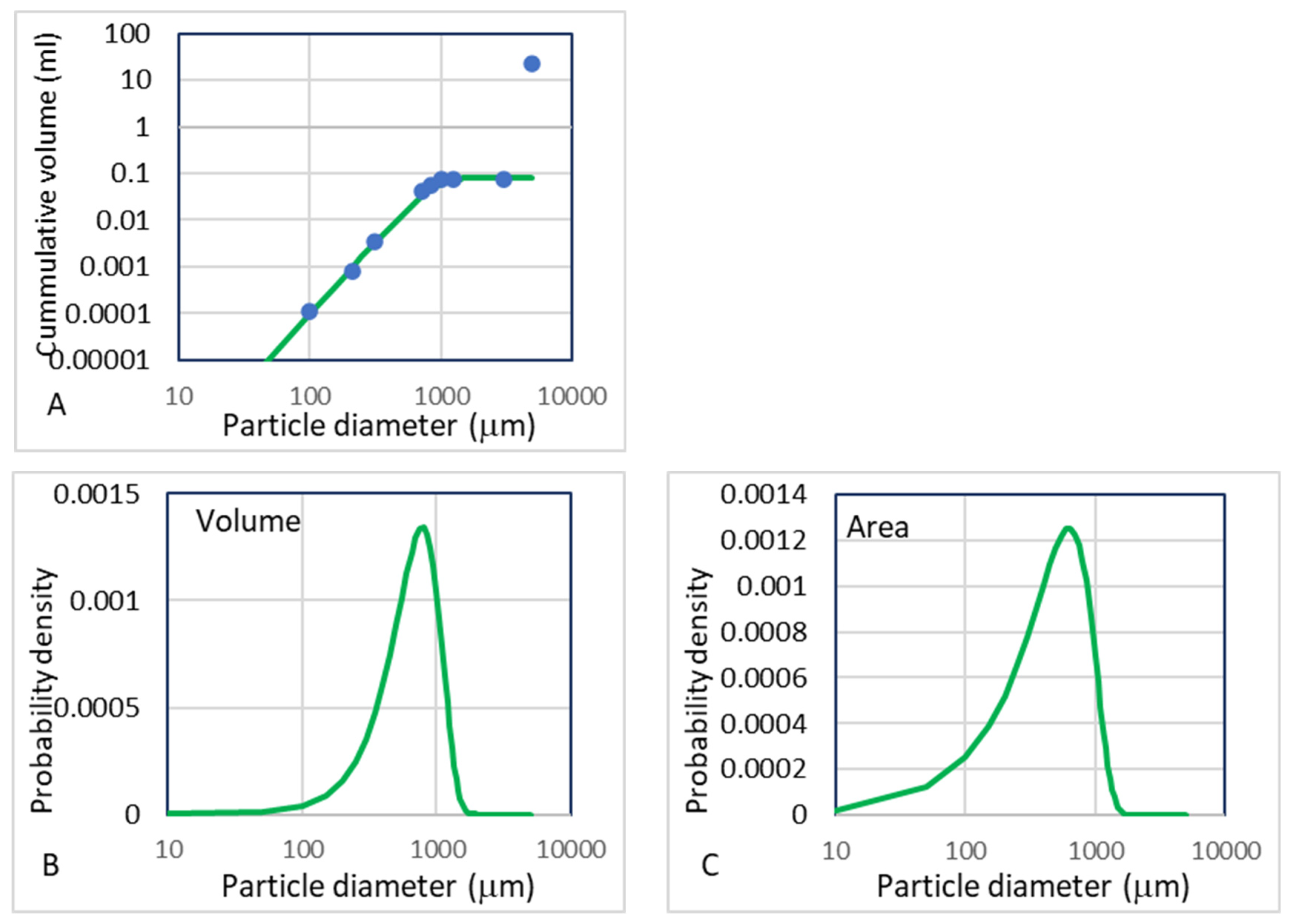
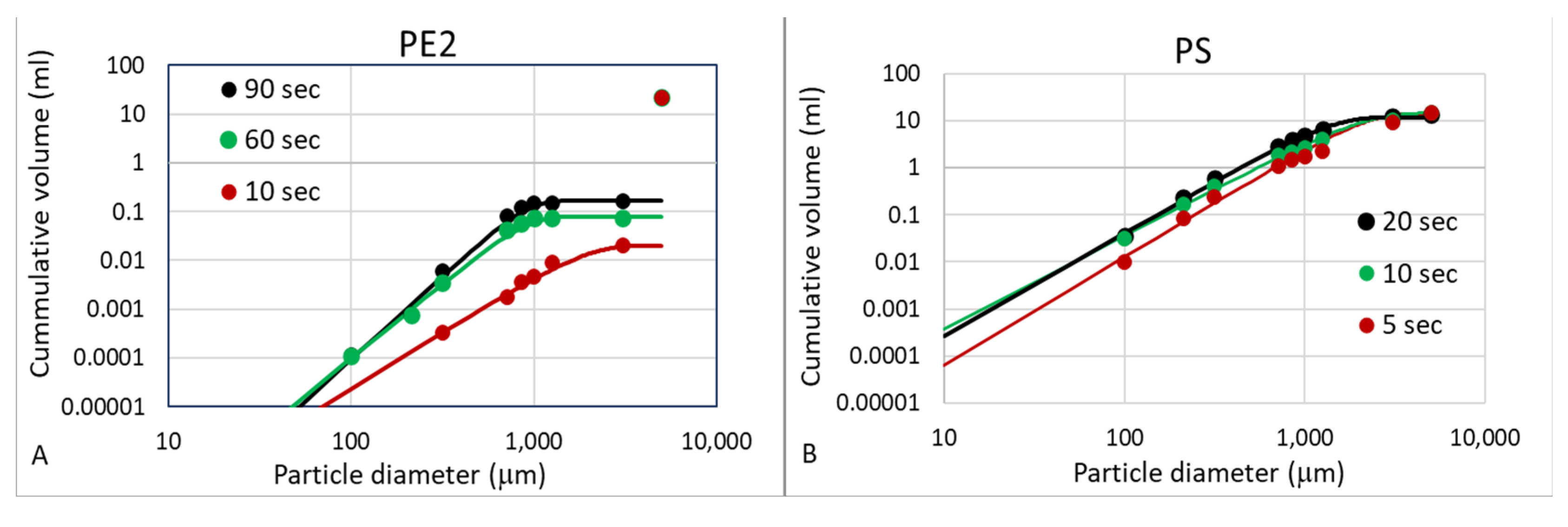
Twenty grams of polymer pellets was milled with an IKA M20 Universal mill, equipped with a star-shaped cutter and an energy use monitor (Voltcraft SEM6000). This method enabled the correlation between energy input for milling and the fracture surface that was generated. The fracture surface was calculated from the particle size distribution of the resulting ground pellets. Twenty grams was taken to submerge the cutter fully. This experiment was conducted for each polymer in three time steps ranging from 10 to 300 s, depending on the type of polymer. The particle size distribution was measured using a set of laboratory sieves (Retsch) having a mesh size between 50 and 3000 μm. The milling time was taken as short as possible to prevent heating of the polymer, which would distort the assessment of the fracture surface energy. Each polymer sample was milled three times, yielding three different particle size distributions. The cumulative volume distribution obtained from the sieving was fitted with a Weibull distribution function. From this distribution, the total volume of microplastics per J, generated by the milling experiments (VI) that can be compared with the calculations of Equation (5), can be calculated according to:
V I = V M I L L δ I E V 0 6 x β λ x λ β 1 e ( x λ ) β d x
λ and β are the distribution parameters of the Weibull distribution, and x is the size of the particles. VMILL is the total volume of polymer that is reduced in size by the milling procedure. EV is the energy input during the milling experiment (J), and δI is the typical particle size from impact stress (according to Equation (1)). The derivation of Equation (17) is explained in Appendix B.

3.4.3. Static Light Scattering

The size and size distribution of the polymer particles were characterized with a Shimadzu SALD7500 nano static laser scattering analyzer, equipped with a SALD-BC75 batch cell and a stirring plate. The polymer particles were measured in ethanol and kept in suspension through constant stirring. To calculate the particle size distribution, refractive indices of 1.50 + 0.00i, 1.55 + 0.00i, 1.60 + 0.00i, and 1.55 + 0.00i were used for PP, PE, PS, and PET, respectively. Deviations from these values may lead to small errors in the calculated particle sizes. For each of the experiments, a distribution of particle sizes is generated. In general, the average particle size decreases during milling and sanding when smaller mesh filters or finer grits are used. However, it was found that the smallest particles in each experiment had a more or less constant size, independent of the mesh or grit size. For the comparison of the polymers, the smallest particle sizes that are produced in relevant quantities during the processes of milling and sanding need to be assessed. Since we do not want to include the very low amounts of small particles that may be accidentally formed by variations in the processes or defects in the materials, the characteristic particle sizes are derived from the number average particle size (DN) as calculated from the particle size distribution given by the static laser scattering analyses, which is calculated according to:
D N = D n x n x n
where Dn and xn are the diameter and number fraction of the nth particle size.
If the fraction of larger particles after milling or sanding is high, the value of DN is shifted to a higher value, which may not represent the actual size of the smallest particles. Therefore, the modal diameter (DM) is also calculated from the number distribution.

4. Results

The required polymer properties of the ten polymers for the theoretical determination of the particle size and volume of MPs, along with results from the actual formation experiments, are given below.

4.1. Mechanical and Physical Material Properties

The measured properties of all ten polymers are listed in Table 3. The E modulus (E), yield strength (σY), ultimate tensile strength (σU), and elongation at break (εU) are derived from the stress–strain curves from the tensile tests. The hardness (H) is measured by the micro-indentation experiment, the shear strength (σS) is calculated from the hardness (=0.0038H2), the notched Charpy impact energy (CN) is derived from the impacts tests, ν is taken from the virgin materials as given by the supplier and assumed to be constant for a polymer type, the surface tension (γ) is measured by the contact angle measurements, and the critical stress intensity factor (KIC) is derived from notched tensile tests. All experiments were conducted at room temperature and were compared with milling and sanding experiments that were also performed at room temperature, thus reducing any temperature effect.
When comparing the tensile results of the two sample sizes, all results (modulus, yield strength, ultimate strength, and elongation were within 10% difference, except for the ultimate elongation of PPHom. Apparently, the processing conditions (mainly cooling rate) differed enough to change the material properties and cause a significant difference in ultimate elongation (11.6% versus 590%). This difference was most likely caused by a difference in crystallinity. In the calculations executed using these properties to derive the MPI values, both εU values were included.

4.2. Calculation of Theoretical Particle Size and Volume of Microplastics during Impact and Wear

The polymer properties given in Table 3 allow for the calculation of the theoretical values for the particle size and volume of the microplastics generated during impact and wear. The results of these calculations are listed in Table 4. This table includes the standard deviations calculated from the standard deviations in the measured properties given in Table 3.
Table 4 shows that particle sizes of the microplastics obtained from impact stresses (milling) are significantly larger than those from wear (sanding and abrasion). Also, the volume of produced particles during impact is much higher for impact than for wear. As mentioned above, for the polymer PPHom, we calculated two values for the microplastic volume of impact and wear. For the higher value of εU, the calculated volume of formed microplastics is significantly smaller for both impact and wear.

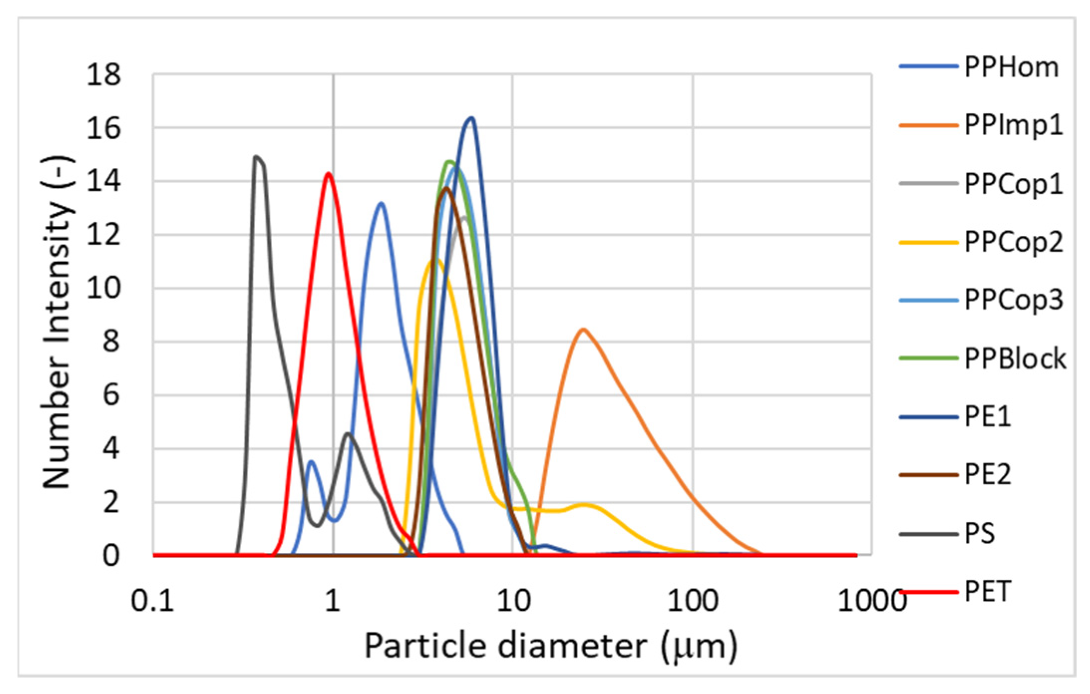
4.3. Experimental Particle Size and Microplastic Formation during Wear

For the assessment of the particle size and volume of formed particles during wear, abrasion experiments were performed with various sanding grit sizes, applied weights, and durations. An example is shown in Table 5 and Figure 3 for the PPHom polymer. In this example, six sanding grits, three weights, and seven sanding times were used. When plotting the calculated wear rate (k) versus the grit density (n) on a log-log scale, Figure 3 was obtained.
This figure shows that all measurements can be found in a single straight line. The various experimental parameters (grit, weight, and time) are included in the two parameters k and n. When fitting these experiments with Equation (16), the wear parameters for each polymer can be obtained. The last (green) point in Figure 3 is the extrapolated value of k at the grit density of 6,250,000 of polished steel. The results of all polymers are shown in Figure 4. It is clear that the polymers PS and PET deviate from the polyolefins. The graphs for the polyolefins seem to cross at a specific grit density of approx. 30,000/mm2. The explanation for this crossover was not found yet.
The microplastics that were generated by the abrasion experiments were measured by SLS. The coarsest sanding paper yielded the largest particles. However, when the grit density of the sanding paper increased, there was no constant decrease in particle size: the smallest particle size appeared to reach a constant value. The particle size distributions of these smallest achievable fractions for all polymers are shown in Figure 5. For some polymers, the smallest particles were found for the #1000 grit, and for others, these were found for the #2000 grit.
Since the whole assessment of the formation of microplastics was aimed at the formation mechanism of the smallest particles, the number distributions were plotted in Figure 5. These figures were used to obtain the number average particle size (DN), and the modal particle size (DM) of the various distributions. The results of the abrasion experiments are summarized in Table 6.
DM seems to be the particle size that represents the smallest value the best. The DN parameter is an average that also includes the particles in the distribution having a substantially larger size. If there is a second peak in the distribution, e.g., for PPCop2 or PS, the difference between DN and DM becomes large, and DN does not represent the smallest fraction anymore. Therefore, the value of DM is used in all future comparisons between experimental and theoretical particle sizes.

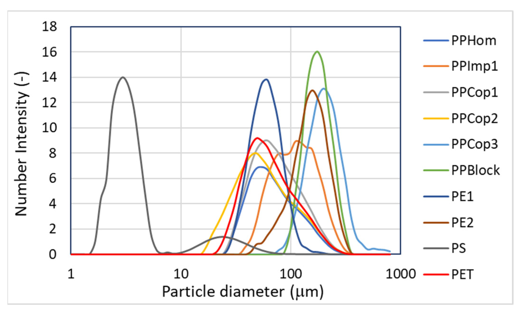
4.4. Experimental Particle Size and Microplastic Formation during Impact

The impact experiments were executed by using two milling tools: the Retsch ZM100 centrifugal mill and the IKA M20 universal mill. The milling experiments using the Retsch mill were used to obtain the particle size distributions. Just like for the abrasion experiments, the number-based particle size distributions of the polymers that were milled by the Retsch ZM100 centrifugal mill were used to obtain the smallest particle fraction that was generated. The particle size distributions of all polymers are shown in Figure 6.
The mesh that was used to separate the ground particles in the mill was 250 μm. This meant that only particles smaller than 250 μm could be collected. Figure 6 clearly shows that the generated particles for most polymers were substantially smaller than 250 μm, indicating proper brittle fracture of the polymer pellets. It is clear that there is a particle size range in the number distribution, and several average particle sizes could be selected for the validation of the model. As was performed for the wear case, two values for the average particle size were calculated: (1) the maximum value of the peak or modal average (DM), and (2) the DN as calculated according to Equation (18).
Retrieving the impact rate, VolμP/J as required in Equation (2) was more difficult than the wear rate. After the grinding of the polymers in the IKA M20 universal mill, two parameters were obtained for each experiment: (1) the amount of energy consumed during the milling; and (2) the cumulative particle size distribution derived from the sieving results. Sieving particles through a sieve stack resulted in a weight- or volume-based distribution. Since the energy for fracture is normally given in J/m2 (see also [14]), we calculated the surface area that was created during the grinding from the particle size distribution. First, the particles passing through the sieve stack were converted from weight into volume, using the density of the polymers. An example of the cumulative volume distribution of PE2 is shown in Figure 7A. The particle size in the figure is the dimension of the holes in the various sieves in the stack. The measured points were fitted to a Weibull distribution curve according to Equations (19) and (A6):
C V = V M I L L 1 e ( x λ ) β
VMILL is the volume of polymer that is affected by the milling procedure and passed through the sieve stack. The point at 5000 μm having a cumulative volume of 14 mL is the total starting volume of the polymer pellets. In Figure 7A, the value of VMILL is approx. 0.1 mL.
The next step was the conversion of the cumulative distribution to a probability volume density function (Equation (A7)) by taking the derivative of the cumulative fit (Figure 7B). Then, the probability area density function was derived by using a correlation between the fracture volume and fracture surface area of the microplastics formed, according to Equation (A9), assuming the particles to be considered as spheres (Figure 7C).
Then, by integrating this area distribution function between 0 and the size of the starting pellets (~5000 μm), the total surface area of the fractured microparticles was calculated, according to Equations (20) and (A10).
C A = V M I L L 0 x = 5000 6 x β λ x λ β 1 e ( x λ ) β d x
In the calculation of the theoretical particle size and volume using Equations (1) and (5), the smallest possible size and corresponding volume were used. This means that for comparison with the experimental results, the microplastic volume having the smallest particle size (DM) should be used. So, for the conversion of the fractured surface area from Equation (20) to a fracture volume rate of VolμP/J as required in Equation (2), we multiplied the fractured surface area with the smallest particle size measured, DM, obtained from the SLS measurements. The volume of impact particles (VI) per J of impact energy (EV) becomes:
V I = C A D M / E V
The grinding and fractionation of the polymers were performed in triplicate to assess reproducibility and to establish a dependency on milling time (if present). Although there were some differences between the three milling times, there was no real trend (see Supplemental Information S1), and the results in Table 7 are an average of the three experiments. Two examples of the cumulative particle distributions are shown in Figure 8 for PE2 and PS. These are representative of the distributions observed for all polymers.
From these cumulative particle size distributions, VI was calculated using Equations (20) and (21). The values for the number average particle size (DN) and modal particle size (DM) were derived from the graphs in Figure 6. All these parameters are listed in Table 7. An overview of all experiments used in the calculation of the average values of VI is listed in Supplemental Information S1.
The calculations to obtain Table 7 values were performed assuming the particles were spheres. If this was not the case, the calculated values changed slightly. When the particles that are formed are more like prolate spheroids, the calculated fracture surface area becomes smaller. When they are more like oblate spheroids, the calculated fracture surface is larger. However, even when these spheroids are very elongated (e.g., length is 10 times the diameter) the difference in calculated fracture surface is ca. 20%. Only in the case of oblate spheroids, when the length is more than 4 times smaller than the diameter, the calculated fracture surface area can become more than 2 times higher. This could explain the differences found between the experimental and theoretical impact volumes as shown in Figure 9B. Apparently, most particles formed resemble the oblate spheroid shape, which means that the experimental results should be a little higher than calculated assuming spherical particles.

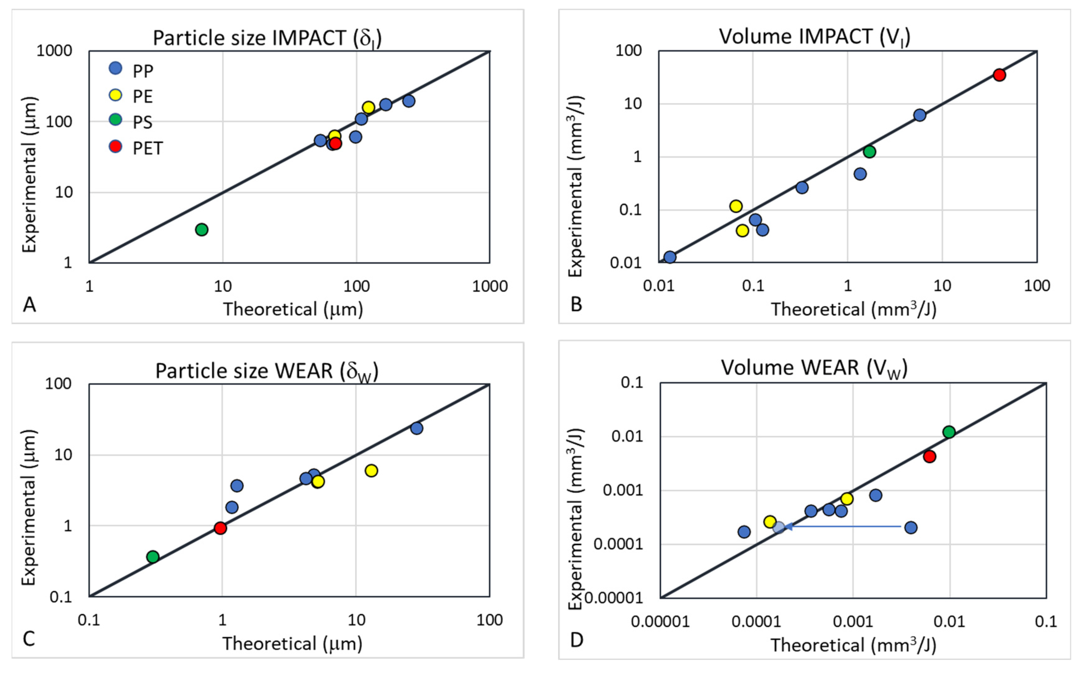
4.5. Comparing Theoretical and Experimental Particle Size and Volume

In the previous sections, the theoretical and experimental particle size and volume of microplastics were obtained for the two cases of impact and wear. These are shown in Figure 9 using the theoretical data presented in Table 4 and experimental data presented in Table 6 (impact) and Table 7 (wear).
With the exception of some points for which the theoretical value deviates significantly from the experimental value, most of the data are well positioned on the 1:1 line, as indicated in Figure 9. A large part of the difference between experimental and theoretical results is caused by cumulative experimental errors. Another significant part of the errors is introduced in the calculations of the volume of impact and wear due to the assumption of spherical particles, whereas in reality, particles will be nonspherical, which can introduce an error as large as a factor of two. The only point in Figure 9 that shows a very high difference between experiment and theory is the PPHom in Figure 9D. However, we already noticed that there is a large difference in εU for the PPHom polymer. When using the value of 590% instead of 11.6%, the point in Figure 9D () moves to the 1:1 line, and matches the experimental value almost exactly. Apparently, the samples used in the wear experiments resembled the small dog bone samples more than the rectangular samples. This could be caused by the change in crystallinity during the processing of the samples. Most polyolefin materials had similar crystallinities for the small dog bone samples as for the larger rectangular bar. However, the crystallinity for the PPHom was 10% higher for the rectangular bar than for the small dog bone, which may have resulted in a material with a lower ultimate elongation. The crystallinity was calculated using the melting enthalpies as given by Grigorescu [20]. Details about the crystallinity measurements can be found in the Supplemental Information S2.

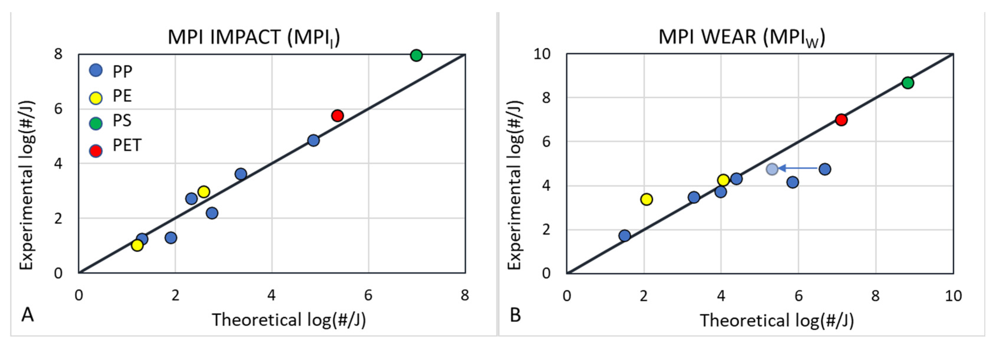
4.6. Comparing Theoretical and Experimental MPI

The final assessment of the tendency for polymers to form microplastics is given in the calculation of the MicroPlastic Index (MPI). This parameter relates to the number of particles that are generated per J of applied energy, as calculated according to Equations (2) and (4). The MPI values calculated from the theoretical and experimental polymer parameters are listed in Table 8.
For a better comparison between the theoretical and experimental values of the MPI, the results are graphically represented in Figure 10.
The experimental MPI for both milling (impact) and sanding (wear) microplastic formation correlates quite well with the theoretical values. Some values deviate more (e.g., PPHOM for wear), which is a logical consequence of the larger errors found in the individual values for δW and VW for these polymers. When using the value of 590% for εU, the MPI for PPHom moves along the arrow to the point and is in much more agreement with the experimental value.

5. Discussion and Conclusions

This paper demonstrates the validity of the MPI model that we presented in an earlier paper [14]. Eleven polymer properties were measured or calculated and subsequently used to calculate the theoretical microplastic particle size and volume formed by the application of impact or wear stresses. These two parameters were experimentally measured using novel testing and measurement techniques developed to facilitate the assessment of the MP formation via both mechanisms.
For both the impact and wear mechanisms, PS and PET show the highest MPI of the polymers tested, which corresponds to the high volume and small particle size of microplastics being produced. The polyolefins show a wide range of fracture behavior for both the particle sizes and microplastic volume. This is caused by the large range of physical and mechanical properties found. PP homopolymer, which combines a high stiffness, hardness, and strength with a low elongation at break, shows a much higher MPI than, for example, a PP copolymer with a lower stiffness and strength and a higher ultimate elongation. The PEs show similar behavior as the PPs.
The large differences observed between the six PP grades and two HDPE grades are important as this shows that it is not only the plastic type that plays a role in MP formation but also the grade/formulation. Polymer grades are often tailored to specific applications; therefore, it could be that plastic from certain applications is more prone to form MPs than others. For example, of the grades tested in this study, the PP used in automotive bumpers is much less prone to forming MPs (through impact and wear) than the grade used for food packaging. In this way, the MPI may help identify applications or sectors of high importance, which are responsible for a large amount of microplastics, thereby also being a tool for exposure and risk assessment. In this case, the MPI may also be used to help reduce MPs. For example, if a number of different grades can be used for the same application, producers will be able to make an informed selection of which has the lowest MP-forming potential. However, this was demonstrated for a small range of polymers and may not be representative of all grades used for a certain application.
The two experimental MP formation testing techniques also offer a simple method for determining the MPI of a material. The polymer properties required to calculate the MPI are not always available on material data sheets, and more importantly, these properties may change upon processing of the material (e.g., injection or blow molding, extruding, etc.). Furthermore, it is not always possible to test these properties on a material in product form. Therefore, these tools offer a practical method for determining the MPI of products.
The use of the MPI model and experiments has the potential to reduce the formation of microplastics from plastic products over their entire lifecycle:
  • During processing: Processing conditions can affect the polymer structure (e.g., crystallinity) and may lead to degradation during extrusion, etc. Changes in polymer properties during processing into a final product may also change the microplastic formation and can be validated by the MPI model.
  • Aging: The chemical changes such as cross-linking and/or decrease in molecular mobility and, thus, mechanical properties change with aging. This means the MPI also changes with aging. We expect that the MPI is also valid for aged material and, thus, could be used to predict the microplastic release of aged plastic material.
  • Recycling: During (multiple) recycling of polymers, degradation of the polymers will occur. The severity of degradation and, therefore, the change in the MPI will depend on the quality of the plastics, the intensity of the processing, and the post-processing steps.
With respect to the health implications of MPs: In the first paper [14], we showed that the abundance of microplastics in the environment correlates with the amount of microplastics that can be expected from a polymer based on the MPI. This opens up the potential to apply the MPI as a tool to better model microplastic emissions and exposure of ecosystems and humans to microplastics. This could be a highly relevant tool for risk assessment of microplastics.
The MPI is used for the calculation of the number of particles formed per Joule of input energy into a polymer. This energy transferred to the polymer can be utilized during processing (e.g., shredding or pelletizing), use (e.g., car tire wear or opening food packaging), or in the environment for littered plastic waste exposed to waves and wind. Knowing these energy inputs, we can estimate the number of particles formed and use this to model the efficiency of mitigation measures that are aimed at process or material modifications.
Another interesting result of this research is the difference in the effect of impact and wear stresses. From the results of the different polymers, it can be concluded that some polymers are more resistant to impact than to wear—e.g., PE1 has a higher MPI for wear than for impact, whereas PE2 has a higher MPI for impact than for wear. This would indicate that PE1 should be used in impact applications and PE2 in applications where more abrasion is to be expected.
The polymers that were addressed in this paper were all amorphous or semicrystalline materials. A possible limitation of the MPI model could be rubbery materials, for which some of the properties are difficult to measure (e.g., impact strength). We will assess the feasibility of the model for rubbers in a forthcoming paper. Future research will also include the effect of aging and degradation, the presence of additives, and processing conditions on the microplastic formation.
We have demonstrated and experimentally validated that the MPI offers a unique way to determine and quantify the microplastic formation of polymers. Its demonstration of large differences between grades of the same polymer highlights the importance of formulation and processing in future efforts to combat MPs. The possibilities to determine the MPI both theoretically and experimentally offer options for all stakeholders in the plastics chain—producers, processors, consumers, and legislators—to take action toward a more circular plastics economy.

Supplementary Materials

The following supporting information can be downloaded at: https://www.mdpi.com/2673-8929/2/4/27/s1.

Author Contributions

Conceptualization, A.B.; data curation, K.G., M.G.A.N., M.M.C.V. and A.E.T.; funding acquisition, A.B., S.H. and J.H.U.; investigation, K.G. and M.G.A.N.; methodology, A.B.; supervision, A.B., S.H. and J.H.U.; validation, K.G. and A.B.; writing—original draft, A.B.; writing—review and editing, K.G., M.G.A.N., L.A.P., S.H. and J.H.U. All authors have read and agreed to the published version of the manuscript.

Funding

This research received no external funding.

Institutional Review Board Statement

Not applicable.

Informed Consent Statement

Not applicable.

Data Availability Statement

The raw experimental data that are generated for the calculation of the particle size and volume of microplastics and MPI are summarized in the supplemental data or can be requested from the corresponding author.

Acknowledgments

The authors would like to thank LyondellBasell, Sabic, and Dufor for kindly supplying the polymer materials.

Conflicts of Interest

The authors declare no conflict of interest.

Appendix A. Coefficient of Friction

The coefficient of dynamic friction ( μ ) was measured in a custom-made apparatus (Figure A1).
Figure A1. Schematic representation of the setup used for the measurement of the coefficient of friction.
Microplastics 02 00027 g0a1
A piece of polymer of approximately 1 × 1 cm (yellow in Figure A1) was positioned on a rectangular sample of the same material (light grey), which was placed at an angle θ, between a sample and the horizontal plane. For most samples, θ was approximately 24° for an accurate measurement, with the exception of PPIMP1 and PET, which were measured at angles of approximately 34° and 16°, respectively, because of their high and low friction. After the release of the sample, it slides downward. Due to the positioning at an angle, the sample experiences an applied force F a p p and a normal force FN, parallel and perpendicular to the ramp, respectively, which can be calculated according to:
F a p p = m g   s i n θ
F N = m g   c o s θ
where m is the mass of the samples in kilograms and g is the gravitational acceleration constant (9.81 m/s2). The time t it took the polymer piece to slide over a distance of l = 6.4 cm over the polymer ramp was determined by recording the slide with a camera and performing a frame-by-frame analysis. The effective force that forces the mass to move over length l in time t (Feff) in the direction of the movement was calculated according to:
F e f f = 2 m l t 2
The friction force, Ffriction that is experienced by the sliding sample, caused by the friction between the two surfaces, is the difference between the applied force and the effective force:
F f r i c t i o n = F a p p F e f f
Finally, the coefficient of dynamic friction μ can be calculated from Ffriction, and FN:
μ = F f r i c t i o n F N

Appendix B. Weibull Distribution

The cumulative volume distribution that is produced by the milling of the polymers by the IKA M20 Universal mill as obtained from the sieving (CV), was fitted with a Weibull distribution function:
C V = V M I L L 1 e ( x λ ) β
λ and β are the distribution parameters of the Weibull distribution, and x the size of the particles. It was assumed that all microplastics produced by the milling follow this Weibull distribution. VMILL is the total volume of polymer that is reduced in size by the milling procedure. This does not include the pellets that were not affected. Knowing the volume distribution, it is now possible to calculate the number and surface area distributions. The volume probability density function is:
P V = V M I L L β λ x λ β 1 e ( x λ ) β
Assuming spherical particles, the number probability density function is:
P N = V M I L L 6 π x 3 β λ x λ β 1 e ( x λ ) β
And the surface area probability density function is:
P A = V M I L L 6 x β λ x λ β 1 e ( x λ ) β
And finally, the cumulative surface area for this Weibull distribution becomes:
C A = V M I L L 0 6 x β λ x λ β 1 e ( x λ ) β d x
which was used to calculate the total surface area that was created during the milling per Joule of input energy:
A I = C A / E V
in which EV is the energy input during the milling experiment (J). If we want to compare this number with the volume of microplastics generated, as calculated in Equation (5), the surface area should be multiplied by the measured particle size according to:
V I = A I δ I
This leads to the final equation for the total volume of microplastics formed by impact:
V I = V M I L L δ I E V 0 6 x β λ x λ β 1 e ( x λ ) β d x

References

  1. Microplastics. Available online: https://echa.europa.eu/hot-topics/microplastics (accessed on 2 November 2023).
  2. Andrady, A.L. Microplastics in the marine environment. Mar. Pollut. Bull. 2011, 62, 1596–1605. [Google Scholar] [CrossRef] [PubMed]
  3. Ibrahim, S.; Andrea, F. Plastic contamination in agricultural soils: A review. Environ. Sci. Eur. 2023, 35, 13. [Google Scholar] [CrossRef]
  4. Koelmans, A.A.; Mohammed Nor, N.H.; Hermsen, E.; Kooi, M.; Mintenig, S.M.; De France, J. Microplastics in freshwaters and drinking water: Critical review and assessment of data quality. Water Res. 2019, 155, 410–422. [Google Scholar] [CrossRef] [PubMed]
  5. Guerranti, C.; Martellini, T.; Perra, G.; Scopetani, C.; Cincinelli, A. Microplastics in cosmetics: Environmental issues and needs for global bans. Environ. Toxicol. Pharmacol. 2019, 68, 75–79. [Google Scholar] [CrossRef] [PubMed]
  6. Leslie, H.A.; van Velzen, M.J.; Brandsma, S.H.; Vethaak, A.D.; Garcia-Vallejo, J.J.; Lamoree, M.H. Discovery and quantification of plastic particle pollution in human blood. Enviro. Intern. 2022, 163, 107199. [Google Scholar] [CrossRef] [PubMed]
  7. Barcelo, D.; Pico, Y.; Alfarhan, A.H. Microplastics: Detection in human samples, cell line studies, and health impacts. Environ. Toxicol. Pharmacol. 2023, 101, 104204. [Google Scholar] [CrossRef] [PubMed]
  8. Ragusa, A.; Svelato, A.; Santacroce, C.; Catalano, P.; Notarstefano, V.; Carnevali, O.; Papa, F.; Rongioletti, M.C.A.; Baiocco, F.; Draghi, S.; et al. Plasticenta: First evidence of microplastics in human placenta. Environ. Int. 2021, 146, 106274. [Google Scholar] [CrossRef] [PubMed]
  9. Lim, X. Microplastics are everywhere—But are they harmful? Nature 2021, 593, 22–25. [Google Scholar] [CrossRef] [PubMed]
  10. Vethaak, A.D.; Legler, J. Microplastics and human health. Science 2021, 371, 672–674. [Google Scholar] [CrossRef]
  11. The Largest Cleanup in History. Available online: www.oceancleanup.com (accessed on 2 November 2023).
  12. Anagnosti, L.; Varvaresou, A.; Pavlou, P.; Protopapa, E.; Carayanni, V. Worldwide actions against plastic pollution from microbeads and microplastics in cosmetics focusing on European policies. Has the issue been handled effectively? Marin. Poll. Bull. 2021, 162, 111883. [Google Scholar] [CrossRef]
  13. Onyena, A.P.; Aniche, D.C.; Ogbulu, B.O.; Rakib, R.J.; Uddin, J.; Walker, T.R. Governance Strategies for Mitigating Microplastic Pollution in the Marine Environment: A Review. Microplastics 2022, 1, 15–46. [Google Scholar] [CrossRef]
  14. Boersma, A.; Griogoriadi, K.; Nooijens, M.; Henke, S.; Kooter, I.M.; Parker, L.A.; Dortmans, A.; Urbanus, H.H. Microplastic Index—How to Predict Microplastics Formation? Polymers 2023, 15, 2185. [Google Scholar] [CrossRef]
  15. Hammond, M.J.; Fawaz, S.A. Stress intensity factors of various size single edge-cracked tension specimens: A review and new solutions. Engin. Fract. Mech. 2016, 153, 25–34. [Google Scholar] [CrossRef]
  16. Boersma, A.; Soloukhin, V.A.; Brokken-Zijp, J.C.M.; De With, G. Load and depth sensing indentation as a tool to monitor a gradient in the mechanical properties across a polymer coating: A study of physical and chemical aging effects. J. Pol. Sci. B Pol. Phys. 2004, 42, 1628–1639. [Google Scholar] [CrossRef]
  17. ASTM D3702-94; Standard Test Method for Wear Rate and Coefficient of Friction of Materials in Self Lubricated Rubbing Contact Using a Thrust Washer Testing Machine. ASTM International: West Conshohocken, PA, USA, 2009.
  18. Amuzu, J.K.A.; Briscoe, B.J.; Tabor, D. Friction and Shear Strength of Polymers. ASLE Trans. 1977, 20, 354–358. [Google Scholar] [CrossRef]
  19. Meng, H.C.; Ludema, K.C. Wear models and predictive equations: Their form and content. Wear 1995, 181–183, 443–457. [Google Scholar] [CrossRef]
  20. Grigorescu, R.M.; Grigore, M.E.; Iancu, L.; Ghioca, P.; Ion, R.-M. Waste Electrical and Electronic Equipment: A Review on the Identification Methods for Polymeric Materials. Recycling 2019, 4, 32. [Google Scholar] [CrossRef]
Figure 1. Shear strength of six polymers plotted against the square of the hardness.
Microplastics 02 00027 g001
Figure 2. Custom-made sanding apparatus and scheme.
Microplastics 02 00027 g002
Figure 3. Relationship of wear rate (k) with grit density (n) for the polymer PPHom. The green point represents the extrapolated value of k at grit density 6,250,000 for polished steel.
Microplastics 02 00027 g003
Figure 4. Wear rate (k) plotted versus the grit density (n) for all polymers.
Microplastics 02 00027 g004
Figure 5. Number particle size distributions for all polymers sanded using the #1000 or #2000 sanding paper.
Microplastics 02 00027 g005
Figure 6. Number particle size distributions for all polymers milled using a mesh for collecting the ground particles < 250 μm.
Microplastics 02 00027 g006
Figure 7. Data processing of a grinding and sieving experiment on PE2: (A) cumulative volume derived from the sieving experiments; (B) probability density function of the volume distribution; (C) probability density function of the area distribution of the fractured polymer pellets.
Microplastics 02 00027 g007
Figure 8. Cumulative volume distributions for two polymers (A: PE2 and B: PS) after milling three times each (10, 60, and 90 s for PE2; 5, 10, and 20 s for PS).
Microplastics 02 00027 g008
Figure 9. Comparison between the experimental and theoretical values for (A) particle size formed through impact (δI); (B) volume of microplastics formed through impact (VI); (C) particle size formed through wear (δW); and (D) volume of microplastics formed through wear (VW).
Microplastics 02 00027 g009
Figure 10. Experimental values of the MPI plotted versus the theoretical values for impact (A) and wear (B).
Microplastics 02 00027 g010
Table 1. Polymers used in the MPI validation study, including supplier, grade, and MFI.
PolymerGradeMFI *ApplicationNameIMT (°C)
PP Homopolymer60Food packagePPHom230
PP Impact copolymer7.5BumpersPPImp1230
PP Random copolymer0.3PipesPPCop1230
PP Random copolymer1.4 aExpansion tankPPCop2230
PP Random copolymer30HousewarePPCop3215
PP Block copolymer37ContainersPPBlock230
HDPECopolymer10 bBottle capsPE1230
HDPECopolymer0.4 bSoap bottlesPE2230
PSMw = 280,0003.3 cGeneralPS245
PETLower Tm and Tg20 dTrayPET300
* All MFIs are given in g/10 min at 230 °C and 2.16 kg, except a (230 °C/5 kg); b (190 °C/2.16 kg); c (200 °C/5 kg); d (converted from intrinsic viscosity to MFI at 285 °C/2.16 kg). IMT = Injection Molding Temperature.
Table 2. Types of sanding paper used in the abrasive wear experiments.
TypeGrit Size (μm)Fraction of Area Covered by Grit (%)# Grit Particles/mm2
P1201255535
P180826089
P50030.264698
P100018.3802379
P20006.56214,681
P40003.66550,154
steel0.41006,250,000
Table 3. Summary of polymer properties used in the calculation of the particle size during impact and wear. The standard deviation of each parameter is given in parentheses.
E *
GPa
H
MPa
σY * MPaσU * MPaσS MPaεU *
%
CN
J/cm2
νμγ
mN/m
KIC Mpa√m
PPHom1.54 (0.09)96.5 (1.6)40.1 (0.6)43.2 (1.0)35.3 (0.81)11.6 * (2.8)0.27 (0.06)0.43 (0.01)0.31 (0.04)31.4 (3.4)2.57 (0.01)
PPImp10.63 (0.04)36.0 (0.9)15.8 (0.9)61.4 (0.8)4.9 (0.17)371 (33)7.38 (0.26)0.43 (0.01)0.61 (0.03)36.1 (2.1)1.46 (0.03)
PPCop10.65 (0.02)57.6 (0.6) 24.6 (0.2)39.1 (2.6)12.6 (0.18)176 (37)1.76 (0.14)0.43 (0.01)0.36 (0.02)39
(1.9)
1.77 (0.05)
PPCop21.16 (0.0187.8 (1.8)34.7 (0.4)44.9 (9.8)29.0 (0.82)92 (40)0.73 (0.09)0.43 (0.01)0.32 (0.05)30.9 (1.1)2.3
(0.03)
PPCop30.81 (0.02)58.4 (0.6)26.5 (0.4)132 (1.0)12.6 (0.19)702 (147)0.94 (0.08)0.43 (0.01)0.38 (0.04)28.8 (1.6)3.24 (0.67)
PPBlock1.43 (0.06)67.7 (1.8)22.5 (0.2)26.9 (0.4)17.3 (0.66)54.9 (9.8)0.75 (0.05)0.43 (0.01)0.32 (0.02)35.9 (2.6)3.25 (0.09)
PE10.70 (0.02)45.1 (0.1)22.1 (0.3)77.3 (0.4)7.6 (0.03)553 (202)0.63 (0.03)0.46 (0.01)0.38 (0.05)35.7 (1.8)1.46 (0.01)
PE20.69 (0.07)56.7 (0.6)22.2 (0.2)29.1 (0.5)12.2 (0.18)91.9 (21.0)5.8 (1.73)0.46 (0.01)0.26 (0.04)36.1 (0.3)1.94 (0.04)
PS2.34 (0.01)164 (12)46.8 (0.4)48.3 (0.3)101 (11)3.33 (0.34)0.41 (0.07)0.34 (0.01)0.31 (0.02)48.2 (1.0)1.53 (0.04)
PET2.41 (0.01)128
(1)
56.2 (0.3)52.2 (1.5)61.4 (0.46)4.13 (0.23)0.14 (0.04)0.43 (0.01)0.25 (0.02)51.4 (3.5)4.34 (0.57)
* All tensile experiments were performed on rectangular bars of 80 × 10 × 4 mm and dog bone samples of 78 × 4 × 2 mm. The tensile results of the two sample sizes were similar for all polymers, except for the ultimate elongation (εU) for PPHom. This value was 11.6% for the larger sample and 590% for the smaller dog bone sample.
Table 4. Theoretical values and their standard deviations (∂) for the particle size (δ) and volume (V) of MPs generated during impact (I) and wear (W) stresses.
δI (μm)∂δI (μm)VI (mm3/J)∂VI (mm3/J)δW (μm)∂δW (μm)VW (mm3/J)∂VW (mm3/J)
Equation (1)Equation (5)Equation (3)Equation (6)
PPHom *53.73.15.71.91.160.150.00390.0011
53.73.10.110.041.160.150.000170.00006
PPImp1108100.0130.00228.22.90.000360.00004
PPCop197.94.90.1050.0244.820.320.000560.00016
PPCop265.51.60.330.151.270.070.000750.00047
PPCop3245710.1240.0464.200.300.0000730.000018
PPBlock165101.330.275.110.500.001690.00033
PE168.82.30.0660.02413.10.840.000140.00005
PE2123130.0770.0305.230.550.000860.00024
PS6.90.41.700.520.300.030.00980.0012
PET69.512.940.112.70.970.070.00620.0006
* The first row of PPHom is calculated using εU = 11.6%; the second line, for εU = 590%.
Table 5. Experimental parameters for the abrasion experiments of PPHom.
NrGritWeight (N)Time (sec)Distance (m)Polymer Sanded (g)n
(#/mm2)
k
(mm3/Nm)
1#1208.12401060.356350.4604
2#1205.041402120.424350.4408
3#1201.451802750.132350.3694
4#1808.122036.20.075890.2849
5#5008.121802750.1466980.0725
6#10008.123004680.08823790.0257
7#20008.123004680.033146810.0097
8#40008.126009360.03150,1540.0046
9Steel 6,250,0000.00021
Table 6. Summary of the results of the abrasion experiments on the ten polymers where ∂k is the error in the extrapolation of the wear experiments to n = 6,250,000 and ∂DM is the standard deviation of the particle size at maximum intensity.
κζk (mm3/Nm)k (mm3/Nm)DN (μm)DM (μm)DM (μm)
PPHom4.1990.6340.000210.000032.021.870.10
PPImp11.3660.5170.000420.0000144.424.33.70
PPCop11.5970.5230.000440.000025.645.350.25
PPCop20.9350.4930.000420.000029.963.770.29
PPCop35.7950.6660.000170.000025.454.760.21
PPBlock0.2350.3610.000830.000035.694.240.23
PE11.3740.5470.000260.000106.706.010.92
PE20.1950.3600.000700.000145.184.240.23
PS12.920.4460.012070.001751.080.370.02
PET0.1780.2380.004310.000730.720.930.05
Table 7. Calculated values for the volume of particles formed per J of impact energy (VI), the standard deviation in this value (∂VI), the number average particle size (DN), the modal particle size (DM), and the standard deviation of the modal particle size (∂DM).
VI (mm3/Nm)VI (mm3/Nm)DN (μm)DM (μm)DM (μm)
PPHom5.400.7879.254.92.6
PPImp10.0160.0051201115.9
PPCop10.0810.02982.761.73.4
PPCop20.2220.05169.448.92.7
PPCop30.0330.00521619810.9
PPBlock0.3710.0581821769.7
PE10.0640.04862.761.73.4
PE20.0510.0131571578.4
PS1.1220.3436.33.00.3
PET30.53.874.848.92.7
Table 8. Calculated MPI and standard deviations for the theoretical and experimental cases for both impact and wear.
TheoreticalExperimentalTheoreticalExperimental
MPII∂MPIIMPII∂MPIIMPIW∂MPIWMPIW∂MPIW
PPHom *4.850.254.790.086.680.324.780.08
3.140.214.790.085.310.284.780.08
PPImp11.300.291.340.131.490.291.750.16
PPCop12.330.232.820.153.980.263.740.07
PPCop23.340.223.560.115.840.294.170.07
PPCop31.210.430.920.093.280.273.480.07
PPBlock2.760.252.110.094.390.294.320.07
PE12.590.222.720.252.070.273.360.20
PE21.900.311.400.124.060.304.240.10
PS6.610.217.910.158.830.318.670.09
PET5.360.375.700.087.110.267.010.09
* The first row of PPHom is calculated using εU = 11.6%; the second line, for εU = 590%.
Disclaimer/Publisher’s Note: The statements, opinions and data contained in all publications are solely those of the individual author(s) and contributor(s) and not of MDPI and/or the editor(s). MDPI and/or the editor(s) disclaim responsibility for any injury to people or property resulting from any ideas, methods, instructions or products referred to in the content.

