Article

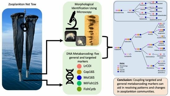
Evaluating Metabarcoding Markers for Identifying Zooplankton and Ichthyoplankton Communities to Species in the Salish Sea: Morphological Comparisons and Rare, Threatened or Invasive Species

1
Smithsonian National Museum of Natural History, Department of Vertebrate Zoology, Washington District of Columbia, Washington, DC 20560-7012, USA
2
School of Oceanography, University of Washington, Seattle, WA 98195, USA
3
Cooperative Institute for Climate, Ocean, and Ecosystem Studies, University of Washington, Seattle, WA 98105, USA
4
Pacific Marine Environmental Laboratory, National Oceanic and Atmospheric Administration (NOAA), Seattle, WA 98115, USA
*
Author to whom correspondence should be addressed.
DNA 2024, 4(1), 1-33; https://doi.org/10.3390/dna4010001
Submission received: 2 October 2023 / Revised: 25 October 2023 / Accepted: 5 December 2023 / Published: 22 December 2023

Abstract

:
Zooplankton and ichthyoplankton community assessments depend on species diagnostics, yet morphological identifications are time-consuming, require taxonomic expertise, and are hampered by a lack of diagnostic characters, particularly for larval stages. Metabarcoding can identify multiple species in communities from short DNA sequences in comparison to reference databases. To evaluate species resolution across phylogenetic groups and food webs of zooplankton and ichthyoplankton, we compare five metabarcode mitochondrial (mt)DNA markers from gene regions of (a) cytochrome c oxidase subunit I, (b) cytochrome b, (c) 16S ribosomal RNA, and (d) 12S ribosomal RNA for DNA extracted from net tows in the Northeastern Pacific Ocean’s Salish Sea across seven sites and two seasons. Species resolved by metabarcoding are compared to invertebrate morphological identifications and biomass estimates. Results indicate that species resolution for different zooplankton and ichthyoplankton taxa can markedly vary among gene regions and markers in comparison to morphological identifications. Thus, researchers seeking “universal” metabarcoding should take caution that several markers and gene regions likely will be needed; all will miss some taxa and yield incomplete overlap. Species resolution requires careful attention to taxon marker selection and coverage in reference sequence repositories. In summary, combined multi-marker metabarcoding and morphological approaches improve broadscale zooplankton diagnostics.

Graphical Abstract

1. Introduction

1.1. Zooplankton Community and Approach

Zooplankton and ichthyoplankton species are distributed unevenly across marine and aquatic ecosystems, in which their relative species’ compositions, numbers, presence, and survival are often highly sensitive and responsive to environmental conditions [1,2,3]. These species frequently interact together, accentuating or dampening the effects of environmental stressors on one another. Notably, coastal zooplankton and ichthyoplankton communities are regarded as some of the most vulnerable to ocean acidification (OA), hypoxia (H), and warming [4,5,6] and are subject to other environmental, chemical, physical, and biological fluctuating conditions (e.g., [7,8]). Moreover, their larval stages often lack species-level diagnostic morphological characters, precluding their identifications using microscopy and other morphology techniques [9,10,11,12,13]. Thus, DNA sequences often provide an important means to identify the species in these communities [11,12,13,14].
In many coastal areas around the world, including the Salish Sea in the temperate Northeastern (NE) Pacific region (Figure 1), zooplankton and ichthyoplankton diversity levels and the ranges of environmental conditions they encounter are high [6,15,16]. The Salish Sea (which includes the Strait of Georgia, the Strait of Juan de Fuca, and Puget Sound) is one of the most biologically rich and diverse inland seas, housing about 260 fish species and more than 3000 invertebrate species [15]. These species are adapted to a broad range of physical and chemical conditions, including salinity, temperature, pH, and dissolved oxygen levels that can fluctuate extensively with season, rainfall, tidal influences, land run-off, and other variables [6,15,16]. Because of its relatively low freshwater inputs and deep (>100 m) water column in many areas, the Salish Sea supports a diverse zooplankton and ichthyoplankton community assemblage that is more representative of coastal and oceanic regions than characteristic of most estuaries [6]. This high zooplankton and ichthyoplankton species diversity distinguishes the Salish Sea from other estuarine ecosystems that have been the focus of most hypoxia and OA studies, making it challenging to fully assess the community diversity using traditional morphological methods. These species diversity levels are relevant because a wide variety of life history strategies, trophic roles, behaviors, and body sizes are represented in the plankton communities, allowing for complex interactions among them, their environment, and their predators. Given that the effects of OAH on trophic interactions are species-specific [5,6], these stressors likely exert a wide range of effects on zooplankton and ichthyoplankton communities.
Moreover, OA conditions in the Salish Sea are commonly at or beyond those regarded as deleterious by the United Nations’ Intergovernmental Panel on Climate Change (IPCC) [17,18,19,20,21]. For example, pH levels <7.6 have become common during the summer in some areas of Puget Sound, with extremely low values (<7.3) observed in its Hood Canal [20,21] (Figure 1, sites F and G). These extreme conditions, together with their highly regional patterning [6,16,20,21], provide a unique opportunity to learn about the effects of changing water chemistry and environmental interactions on planktonic organisms. To help address this, the present study places particular focus on copepods and other crustacean, mollusk, and ichthyoplankton species, since field and laboratory investigations have indicated that these taxa are often sensitive to OAH and other environmental perturbations [16,17,18,19,20,21,22,23,24].
The various species comprising zooplankton and ichthyoplankton communities are not ecologically interchangeable, often respond differentially to environmental stressors, and may occur at various times and places [7,8,10,11,12,13]. In other words, these are dynamic communities upon which other organisms depend for food [25,26,27], and they are critical to ecosystem services and seafood resources [12,13,16]. However, the sheer numbers of plankton samples required, and the diverse taxonomic coverage needed to identify their component species and monitor such complex community changes are prohibitive using traditional morphological analyses alone (see [12,28,29,30]).

1.2. Metabarcoding Markers Evaluated for the Zooplankton and Ichthyoplankton Communities

Our research aims to contribute genetic identification methodology, ground-truthed with zooplankton morphological identifications, towards understanding and monitoring the dynamic responses of zooplankton and ichthyoplankton species and their communities in future studies. Here we employ a high-throughput sequence (HTS) metabarcoding assay approach, which prior studies have indicated can capture a broad diversity of taxa that are often difficult to identify using microscopy and/or other morphological techniques; these include many larval bivalves, gastropods, polychaetes, copepods, and fishes [28,29,30,31,32]. Metabarcoding can also detect species that are low in abundance and/or cryptic [3,9,29,30,31,32,33,34,35,36].
Effective metabarcoding gene regions (markers) require an appropriate level of sequence variability to distinguish among species/taxa of interest, and the primers that flank these diagnostic sequences must anneal to conserved sequences on either end [31,32,33,34,35,36]. When the appropriate gene region/marker and primers are selected, the internal sequence region contains nucleotide variants that can be used to distinguish among the species/taxa in a sample in comparison to reference sequence databases [28,29,30,31,32,33,34,35,36].
Researchers thus aim to select the metabarcoding markers and corresponding primers that are most likely to identify the target taxa/species at the desired taxonomic level [13,28,29,30,31,32,33,34,35,36]. However, some markers are limited to higher systematic levels because they lack distinctive sequence variation (i.e., the gene region is either too conserved or the marker length is too short to include enough variant nucleotides), and/or available DNA sequence reference repositories are incomplete [13,31,32,33,34,35,36,37]. Mitochondrial (mt)DNA gene regions have been used to identify invertebrate and fish species because their evolutionary lineage tracing is simpler than that of nuclear genes since mtDNA is usually uniparentally inherited without recombination [38,39,40,41]. Consequently, many mtDNA gene regions are well represented in sequence repositories [3,9,11,13,28,29,30,31,32,33,34,35,36,41]. Also, the overall abundance of mtDNA in multicellular animals often greatly outnumbers that of their nuclear DNA (summarized by [42]), which can facilitate detection of rare species and/or smaller-sized individuals in field samples (see [41]).
One of the more popular mtDNA gene regions for identifying invertebrate and fish species is cytochrome c oxidase subunit I (COI), which was advocated as the “barcode of life” in the 2000s [43]. Consequently, many invertebrate and fish species have been sequenced for COI, yielding high representation in sequence repositories (e.g., [43,44,45,46,47,48,49,50]). Our study evaluates its species identifications in the Salish Sea using the metabarcoding COI marker “LrCOI” designed by Leray et al. (2013) [49] as modified by Geller et al. (2013) [50], which averages 313 base pairs (bp) in length (Supplementary Table S1), has been widely employed for invertebrates from marine and freshwater habitats [13,49,50,51,52], and additionally resolves some fish taxa [49].
Other frequently used mtDNA sequence regions for species/taxon diagnostics of invertebrates and fishes include the two ribosomal (rRNA) subunit genes, 16S and 12S RNA [14,32,36,39,40]. These ribosomal sequence regions overall are more conserved than other mtDNA gene regions, including COI (above) and cyt b (below) [38,39,40,41,53], since many of their nucleotides are critical to the structure and function of the mt ribosomes [41,53,54]. Thus, congeneric species and other relatives can share the same sequences, especially in the short marker regions used in many high-throughput sequencing (HTS) metabarcoding platforms [36,51,52,53,54]. This can be alleviated by using longer-read markers; however, the degraded quality of many environmental (e)DNA water samples often precludes the use of longer markers [37].
Our study evaluates the mt 16S RNA “Cop16S” metabarcoding marker that was designed to identify marine Calanoida Copepoda (Crustacea, Arthropoda) in Tasmania, Australia, by Clarke et al. (2017) and averages about 301 NTs in length [55] (Supplementary Table S1). The original study found that Cop16S also resolved other crustacean species, including Cladocera (water fleas), Euphausiacea (krills), and Decapoda (crabs, shrimps, etc.) [55]. Background data for the present investigation revealed that Cop16S identified copepod and euphausiid species from NE Pacific marine coastal eDNA water samples [56]. In the freshwater Great Lakes, Cop16S identified copepod species and other (but not all) crustaceans [31], illustrating the marker’s broad salinity range utility. The present investigation compares species identifications of Salish Sea invertebrates among the LrCOI, Cop16S, and Mol16S (below) metabarcoding markers.
We additionally evaluate invertebrate species identified by a mtDNA 16S RNA metabarcoding marker called “Mol16S”, which was designed to identify freshwater Mollusca species by Klymus et al. (2017) [36] for use in zooplankton and eDNA water samples. Mol16S further resolved other invertebrate species belonging to diverse taxa, including Annelida (segmented worms), Arthropoda (including Crustacea), Bryozoa (=Ectoprocta; moss animals), Entoprocta (=Kamptozoa), Porifera (sponges), and Rotifera [31,36]. Mol16S ranges from 125–185 bp in length (Supplementary Table S1) and was additionally found to identify some fish species (for which an additional fish “blocker” primer can be added to reduce the fish sequence read signal) (see [36]). Background data for the present study conducted in marine NE Pacific waters showed that Mol16S identified marine Mollusca, Crustacea, Echinodermata, and some fish (Teleostei, Actinopterygii, and Chordata) species from coastal and deep-sea hydrothermal vent habitats with eDNA water samples [56]. This metabarcoding marker’s versatility reflects that the shared evolutionary histories of some invertebrate taxa have encompassed biogeographic movements among marine, estuarine, and freshwater habitats [57], with some species being euryhaline today (see [58]). Our investigation explores the utility of Mol16S to identify mollusks and other taxa in the Salish Sea.
We also analyze the widely-employed “MiFish12S” mt 12S RNA metabarcoding marker that was designed to identify marine Actinopterygii fish species by Miya et al. (2015) [59]. MiFish12S averages about 172 bp in length [59] and has been broadly used across marine to freshwater ecosystems, mostly for eDNA water samples [59,60,61,62,63]; here we evaluate it for companion ichthyoplankton studies (Supplementary Table S1). Our study compares fish species identified by MiFish12S and FishCytb (described next).
Like COI, the mt cytochrome (cyt) b gene evolves relatively quickly, has considerable nucleotide diversity (particularly in the third codon “wobble” position), and a long history of sequencing popularity for fishes and invertebrates, with relatively high representation in repositories (e.g., [39,40,41,62,63]). Our study evaluates a “FishCytb” marker that was originally designed to identify freshwater fish species by Snyder and Stepien (2020a) and by Snyder and Stepien et al. (2020) [62,63]. FishCytb was targeted to differentiate among all native and nonindigenous fish species in the Great Lakes with eDNA water samples and averages 154 bp in length [62,63] (Supplementary Table S1). Preliminary background results also showed its utility in identifying marine fish species in NE Pacific coastal eDNA water samples [background data, CAS]. This marker’s versatility traces to the freshwater evolutionary origin of Actinopterygii fishes (summarized by [64]). Moreover, (a) many fish taxa (including families, some genera, and some species) have moved among marine, estuarine, and/or freshwater habitats during their evolutionary and biogeographic histories [64], (b) some species are euryhaline, and (c) catadromous and anadromous species transverse salinity realms during their life stages (e.g., some salmonid species, including in the Salish Sea) [15]. Our investigation compares fish species identifications among metabarcoding markers.

1.3. Project Aim and Scientific Question

The present study evaluates which zooplankton and ichthyoplankton species/taxa can be identified in the Salish Sea ecosystem by comparing species/taxon identification results from five previously published mitochondrial (mt) DNA metabarcoding markers with traditional microscopic zooplankton identifications. The markers were originally developed for eDNA analyses of water samples, and can be used in companion studies to our zooplankton net tows. Our objective is to help improve species-level identifications by facilitating appropriate metabarcoding gene region/marker choices for researchers and managers. This paper is a prelude to more comprehensive, multi-year, multi-season investigations in this system. Our ultimate aim is to employ this approach towards addressing the question, “How can we best understand zooplankton and ichthyoplankton community compositions, species diversities, and relative abundance fluctuations over time and space across the Salish Sea”?

2. Materials and Methods

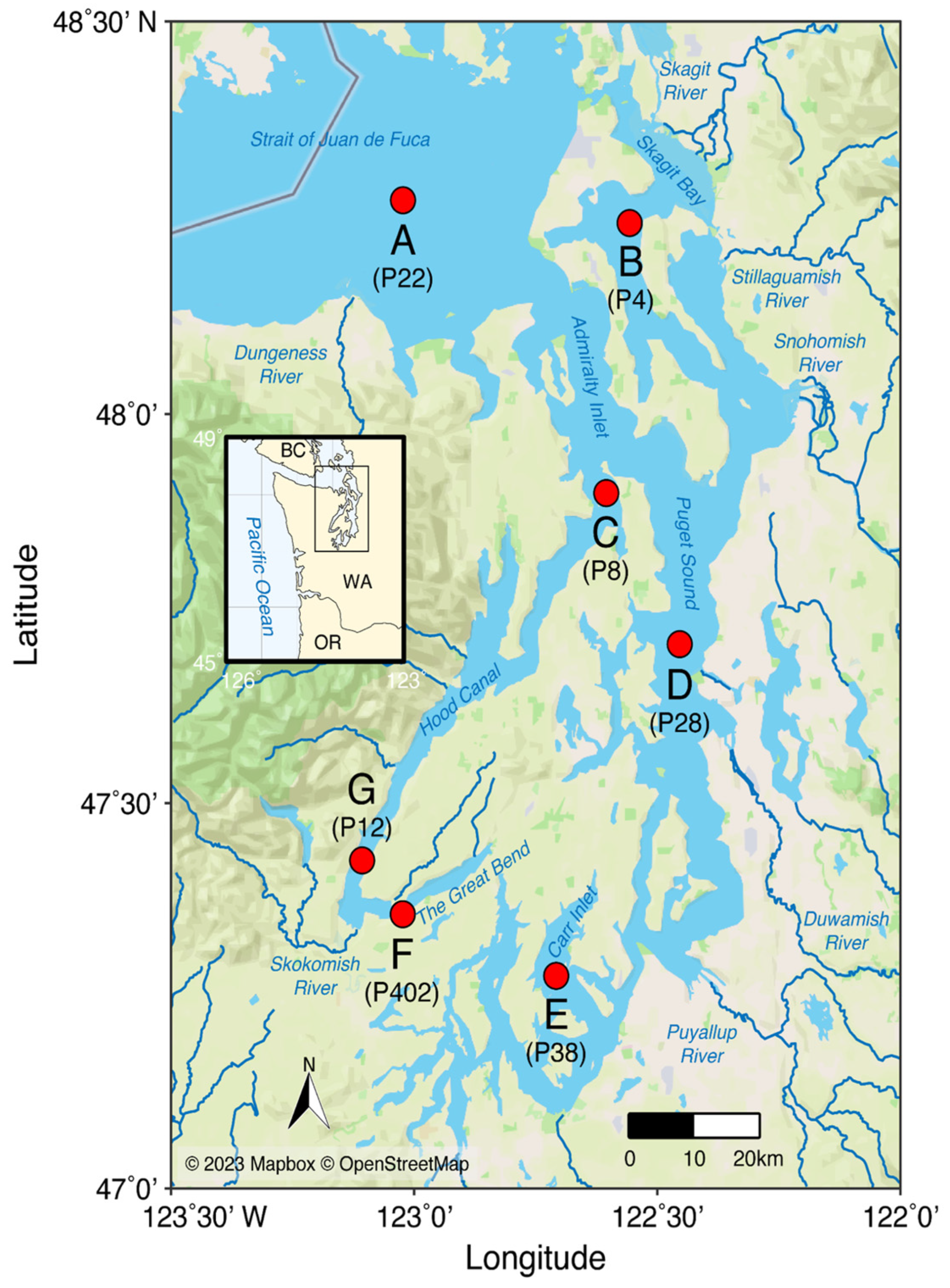
2.1. Sampling, Metadata, and Morphological Identifications

Plankton net tow sampling in the Salish Sea was conducted during Washington Ocean Acidification Center (WOAC) cruises using their protocols, procedures, and permits [16,65,66,67]. We collected zooplankton (including ichthyoplankton) from seven long-term monitoring sites that span a breadth of oceanographic conditions (Figure 1, lettered A–G); here we present findings from spring and autumn 2018. Zooplankton sampling consisted of two net tows at each site: one full-water-column vertical bongo net tow (60 cm diameter, 200 µm mesh) to sample small and relatively weakly swimming taxa, and one full-water-column oblique bongo net tow (60 cm diameter, 335 µm mesh) to sample larger, more mobile taxa (including fish larvae and krills). Tows were conducted without regard to the time of day. Flow meters were used to measure the volume of water filtered. One half of each tow was saved in buffered 5% formalin for microscopic analysis, while the other was preserved in new sterile jars with 95% EtOH for DNA extraction, allowing for direct paired samples to be analyzed by morphology or metabarcoding. For the latter, the sample was re-sieved (sieves were cleaned with a 10% bleach solution and rinsed with sterile ddH2O), and the 95% EtOH was replaced after the cruise due to possible dilution by tissue fluids (per [68]).
Water column physics and chemistry were characterized by WOAC scientists using CTD (conductivity, temperature, and pressure) casts conducted to 10 m above the seafloor. Niskin bottles collected water at 8–12 m depths for laboratory analyses of oxygen, nutrient concentrations (NO3, NO2, NH3, Si(OH)4, PO4), and inorganic carbon chemistry (measurements of dissolved inorganic carbon and alkalinity, for calculation of pH and aragonite saturation state) using WOAC Best Practices [65,66]. Parameters at our net-tow sampling sites are in Table 1. Vertical zooplankton tows were analyzed at every site, and oblique tows were additionally assessed for sites C and E.
Morphological identifications of the zooplankton were conducted using traditional microscopy following [16,66,68,69,70,71,72,73]. First, rare, larger organisms (usually >1 cm) were removed from the entire sample for identification and measurement. When densities were very high, samples were first quantitatively split with a Folsom splitter (Wildco®, Science First®, Yulee, FL, USA). Two 1-mL aliquots were then extracted for analysis from the whole (or split) sample using a Hensen–Stempel pipette (Wildco®, Science First®, Yulee, FL, USA). Finally, a larger aliquot (>10 mL) was taken to quantify mid-sized taxa that had not adequately been subsampled with smaller aliquots. All heterotrophic organisms in the subsamples were enumerated, identified, and differentiated by life history stage when possible using morphological characteristics. A minimum of 400 individuals were identified morphologically from each sample, using taxonomic keys and methodology that are standard to the JEK lab [16,66,68,69,70,71,72,73,74,75,76]. All samples were taxonomically analyzed by two highly-trained taxonomists who have been working on Salish Sea zooplankton for more than a decade. The taxonomists regularly cross-verify species identification between each other, and with taxonomists from outside the laboratory as needed, to maintain consistent, high-quality identifications.
Density (#m−3) was calculated from counts and the volume of water filtered. For small organisms, density was converted to carbon biomass using published values for average carbon per individual. For organisms that varied greatly in size within given life stages, up to 30 individuals were measured per stage and sampled to convert size to biomass using the length: carbon relationship [16,66]. Biomass was the primary morphological metric used for comparisons with the numbers (proportions) of sequence reads from metabarcoding; both numbers of individuals and biomass are reported here for morphology in our Figures and Supplementary Materials.

2.2. DNA Extraction, Library Preparation, and Metabarcoding

For large-volume plankton samples, we used a Folsom plankton splitter (cleaned with 10% bleach and rinsed with sterile ddH20 before and between samples) to quantitatively subsample a 5–10 mL volume, yielding unbiased subsamples in suspension [77], and ground them using a sterile mortar and pestle in sterile CTAB (hexadecyl trimethyl ammonium bromide) buffer (using UV light, laminar hoods, 10% bleach, sterile containers). Genomic DNA was extracted under the above sterile conditions using phenol-chloroform-isoamyl alcohol (following [78]). DNA quantity and quality were checked with 2% agarose mini-gels, a Nanodrop® spectrophotometer (Thermo Fisher Scientific, Waltham, MA, USA), and a Qubit® fluorometer (Thermo Fisher Scientific). Products were cleaned using Qiagen DNeasy PowerClean Pro kits (Qiagen®, Germantown, MD, USDA)
Initial PCR amplifications used 25 µL volumes with 5 µL 5X buffer, 0.25 mM dNTPs, 1.5 mM MgCl2, 0.5 µM of each primer, 0.5 µL (2.5 units) AllTaq® (Qiagen), and 2 µL (10 ng/µL stock) template DNA. PCR amplification conditions were: 30 s at 95 °C, followed by 35 cycles for 5 s at 95 °C, 15 s at annealing temperature (Supplementary Table S1), and 10 s at 72 °C. PCR products were visualized on 2% agarose gels and cleaned using HighPrep™ (Mag BioGenomics®, Gaithersburg, MD, USA) PCR clean-up kits with a 0.7× magnetic bead concentration. Indexing reactions used 25 µL volumes of 2.5 µL 10× buffer, 0.25 mM dNTPs, 1 µM of each primer, 0.313 µL (0.15 Units) Hotstart™ Taq polymerase (New England Biolabs®, Inc., Ipswich, MA, USA), and 3 µL DNA product (10 ng/µL) from the PCR cleanup. Indexing conditions were 30 s at 95 °C, followed by 8 cycles of 30 s at 95 °C, 30 s at 55 °C, and 60 s at 68 °C, with a final 2 min extension at 68 °C. PCR products were visualized and cleaned as above. The length and quality of the final PCR products were determined on a 2100 Bioanalyzer (Agilent Technologies, Inc., Santa Clara, CA, USA).
At each step, negative controls were included to monitor for potential contamination. In spring 2018, we brought sterilized empty containers to the ship, which were opened during plankton transfers, filled with 95% EtOH, and treated the same as the plankton samples (but did not contain plankton). These then served as controls for DNA extractions, along with extraction controls containing reagents only (these were run for all samples). Additionally, two technical PCR replicates were analyzed for the spring 2018 samples in the laboratory, which were analyzed separately to evaluate consistency. PCR controls were also used at each step, which contained only reagents (no DNA).
Five mtDNA metabarcoding markers (see Introduction) were used to identify species/taxa: (a) LrCOI [49,50], (b) Cop16S [55], (c) Mol16S [36], (d) MiFish12S [59], and (e) FishCytb [62,63]. These markers had been previously evaluated in the CAS lab [31,36,56,62,63]. Primer sequences and PCR parameters are in Supplementary Table S1. Our sequencing preparation and procedures followed [31]. All primer sets included Illumina sequencing adapters and four unique spacer inserts at the 5′ end, which served as indices for the initial amplifications [31,36]. These spacer inserts varied from 7–14 nucleotides to offset sequences and increase library diversity, acting to improve the quality of sequence data on the Illumina platform [79,80]. Potential index hops and/or cross-contamination were also reduced by using these spacer inserts (see [62]).
For all MiSeq runs, we used DNA concentrations of 10 pM, measured with a Qubit® fluorometer. A 30% PhiX DNA spike-in was used to enhance the data quality of samples that may have had low nucleotide diversities [31,36,61,62]. Illumina MiSeq runs were performed at the Ohio State University’s Molecular and Cellular Imaging Facility in Wooster, OH, USA (https://mcic.osu.edu/home, accessed on 12 November 2023), and the autumn 2018 samples were additionally run at the Oregon State University’s Center for Quantitative Life Sciences in Corvallis, OR, USA (https://cgrb.oregonstate.edu/bioinformatics, accessed on 12 November 2023) to evaluate congruence. The different markers were run on separate lanes.

2.3. Bioinformatic Processing

Bioinformatic processing was conducted programmatically using REVAMP [81]. Briefly, adapters and amplicon primers were trimmed from the sequence reads using the program Cutadapt (v 3.7 [82]), without length trimming, and with each sequence pair requiring a match to either the forward or reverse primer (respectively). Adapter-trimmed sequence reads were then quality-filtered with DADA2 (v 1.18.0 [83]), using a minimum length of 100 bp, PhiX removal, limited quality truncation (trunQ = 2), and maxEE(5) settings. High quality reads were then run through the DADA2 pipeline to evaluate errors, dereplicate reads, merge read pairs (with a minimum overlap of 20 bp), check for chimeras, and create Amplicon Sequence Variant (ASV) files for ASVs having two or more reads.
To identify the taxon for each ASV, BLASTn [84] was queried against the NCBI (National Center for Biotechnology Information) nucleotide (nt) database [85] (downloaded 12 November 2021), whose output displayed the best “hit” (i.e., sequence match) for up to 4000 target sequences, to circumvent individual taxa that had large numbers of sequenced individuals from dominating the BLASTn results. A negative taxonomic identification (taxID) list excluded taxIDs for which the “scientific name” category included “uncultured”, “environmental samples”, “metagenome”, “unidentified”, or “unclassified” labels, including nodes downstream of those identified using the program Subtree [86]. The BLASTn data were then reformatted to exclude matches less than the designated length cutoffs (300 bp for LrCOI, 100 bp for Cop16S and Mol16S, 140 bp for MiFish, and 120 bp for FishCytb). Only taxIDs with the highest percent identity per ASV were included in taxonomic analyses.
All taxIDs from the BLASTn results were converted to a standard taxonomic hierarchy using Taxonkit [87], which was modified further to fill in gaps in the taxonomic hierarchy by assigning missing values from the next lower hierarchical level that was identified (e.g., an unlabeled family with a known genus would be classified as genus__f). A custom script then parsed all taxID hits for each ASV to determine its best (i.e., closest match) taxonomic assignment (https://github.com/McAllister-NOAA/asv_to_taxonomy, 12 November 2023). Thus, taxonomic choices were based on the deepest common hierarchy shared by all best BLAST hits per ASV, with the final taxonomic depth appropriate to the confidence of assignment based on the percent identity. These confidence rankings allowed hits ≥95% (for protein-encoding genes) and/or ≥97% (for rRNA genes) to be assigned to species level: 95/97% > x ≥ 92/95% to genus, 92/95% > x ≥ 87/90% to family, 87/90% > x ≥ 77/80% to order, 77/80% > x ≥ 67/70% to class, 67/70% > x ≥ 60% to phylum, and any hit <60% was assigned to “unknown.” Reference sequences that were assigned to more than one taxID were purged from the results, unless that reference sequence was the sole best hit for that ASV. Those decisions produced a file that linked each ASV to its taxonomic identity, which was then used for downstream assessment.
Morphological taxonomic data were processed to evaluate concordance with the sequencing data from each marker. Taxonomic IDs were generated using the name2taxid function of Taxonkit [87]. Gaps in the taxonomic hierarchy were filled only when its morphological assignment corresponded to an intermediate taxonomic level (i.e., suborder, superclass), in which case the intermediate taxonomic identification was designated with an appropriate lower-level modifier (i.e., Subclass__f equated to a family classification for the family within that known subclass).

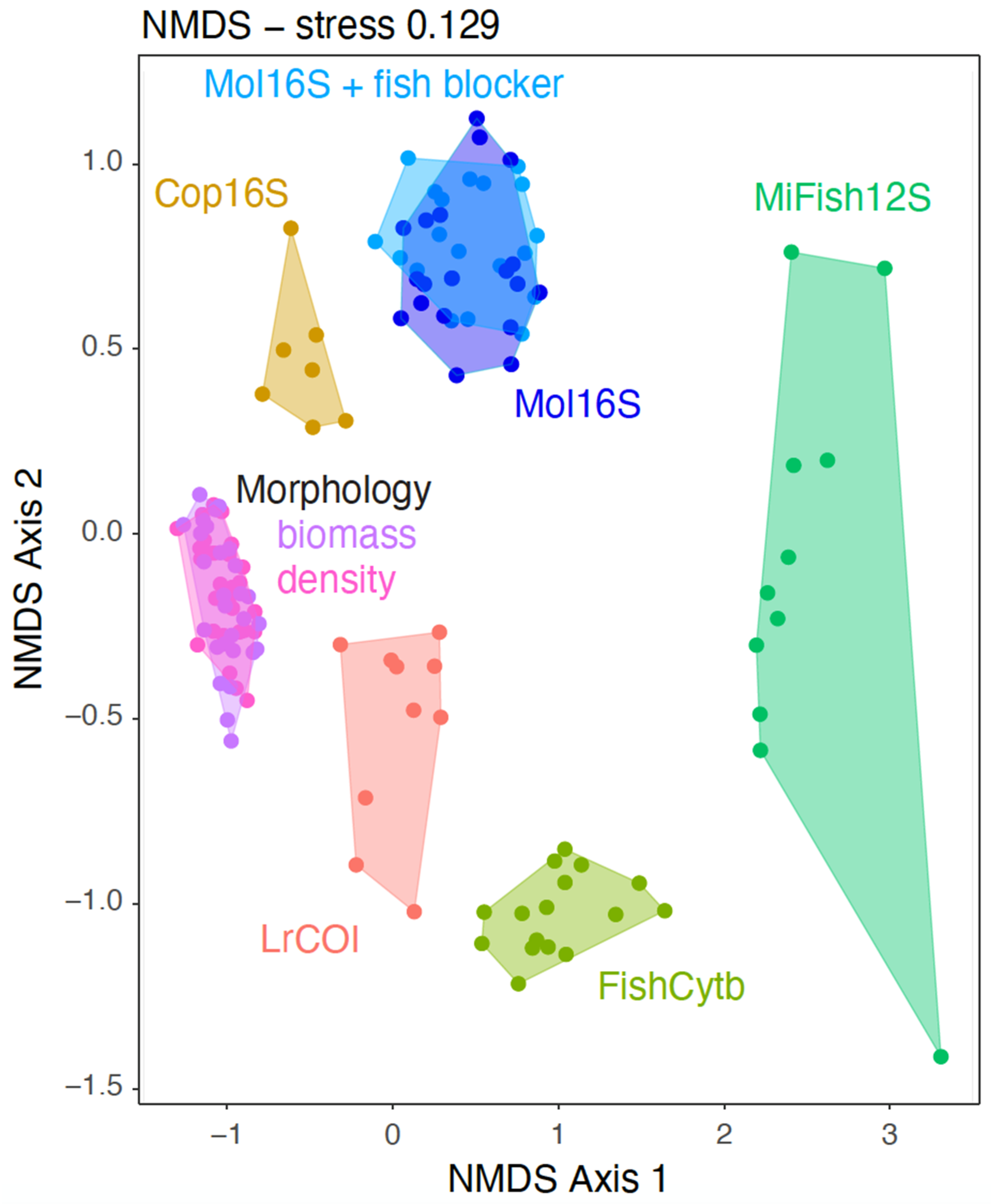
2.4. Statistical Analyses

Relative abundances of species/taxa according to their respective morphological proportions and biomasses, or for sequence read counts, were classified as being either rare (<1%), low (1–3%), moderate (4–10%), or high (>10%) in relative representation. Summary figures showing respective sequence read counts using the interactive taxonomic hierarchy are illustrated with Krona plots [88] in Supplementary Figure S1 (at https://figshare.com/articles/figure/Supplemental_Figure_1/21791738/1). Bar plots depicting respective relative abundances, in which taxa having <5% relative abundances were grouped as “Other”, were constructed using the plot bar function of Phyloseq in R [89]. Multidimensional statistical analyses were conducted for each marker and morphology data based on the relative proportional data (relative abundance, proportional density, proportional biomass) using the nonmetric-multidimensional scaling (NMDS) ordination function in Phyloseq [90], which is a method that is relatively free of assumptions, facilitating visualization of relationships among data sets [90]. Marker and morphology data comparisons were made by first merging identical taxonomic assignments across all comparison datasets. Venn diagrams were created in R [91].
Results from our metabarcoding assays were compared with morphological identifications made from the same (split) sample. Species appearing unique to either the metabarcoding assays and/or morphology were evaluated from these samples and across the sampling locations. The nearest taxonomic levels to which each marker and morphological methods identified the species/taxa were evaluated using network plots using the visNetwork package in R [92]. Biomass proportions of species from morphological identifications and the proportion of sequence reads for single metabarcoding assays were arcsine square root transformed and statistically compared using simple linear regression models and Pearson correlations in R, with probability (p-) values corrected for multiple comparisons and controlled for false discovery rate [93]. Samples for which either the morphological or metabarcoding marker proportions were zero were excluded from analyses.
Assignments of putative nonindigenous species were evaluated in further detail since their indication might invoke a management response (see [9,94]). Their ASVs were examined for two factors: (1) percent identity (PID) to the assigned species/taxon, and (2) whether potential locally occurring species or known nonindigenous species from the Salish Sea or other NE Pacific regions had published sequences for that gene region. Additionally, these ASVs were assessed for: (3) the number of sequence reads, (4) the number of samples in which the ASV was found, and (5) the PID of the next closest assignment. ASVs with a low PID and/or lack of reference data for locally occurring species were considered “low confidence” matches here. ASVs with high PID and local reference data, which additionally had high read counts in numerous samples (high confidence in detection sensitivity and limited probability of detection through sequencing errors), were assigned as “high confidence” matches.

3. Results

PCR amplifications were not found in our negative extractions, centrifugations, no-template PCRs, indexing, or clean-up controls. The two technical replicates run for spring 2018 samples yielded very similar and congruent results. Duplicate DNA extractions and PCR library preps showed comparable results. Supplementary Table S2 provides the total number of sequence reads (paired and single reads post-merge) at each step in the quality control pipeline. Amplicon sequence variant (ASV) counts for each metabarcoding marker are in Supplementary Table S3. These results show that the ASV identifications had at least a median value of 99.4% similarity to the reference sequence database for the markers, ranging from 99.7% for Cop16S to 99.4% for the other four markers. ASV identifications at the genus level ranged from a median of 94.9% (LrCOI) to 99.4% (MiFish12S) (Supplementary Table S3).
Taxa resolved at each classification level per marker, sample, and site are in Supplementary Table S4, along with relative abundances per marker. Krona plots of the taxa are in Supplementary Figure S1. Supplementary Table S5 lists species used for other sequencing studies in the laboratory during the previous three years, indicating those that were found or not found in our results.
The tree diagram in Figure 2 depicts the taxa identified to the level of class by each of the five metabarcoding markers and our morphological identifications for 15 major phyla (in alphabetical order): Annelida (LrCOI, Mol16S, FishCytb, Morphology), Arthropoda (LrCOI, Cop16S, Mol16S, FishCytb, Morphology), Bryozoa (LrCOI, Cop16S, Mol16S), Chaetognatha (LrCOI, Mol16S), Chordata (LrCOI, Mol16S, FishCytb, Morphology), Cnidaria (LrCOI, Cop16S, Mol16S, Mifish12S, Morphology), Ctenophora (LrCOI alone), Echinodermata (all but MiFish12S), Entoprocta (Mol16S alone), Mollusca (all but MiFish12S), Nemertea (LrCOI, Cop16S, Mol16S), Phoronida (LrCOI, Mol16S, FishCytb), Platyhelminthes (LrCOI, Mol16S), Porifera (LrCOI), and Rotifera (LrCOI, Mol16S). The markers and morphology each differentially resolved various taxa within those phyla (Supplementary Figure S1; Supplementary Table S4).
Morphology alone identified members of the Chordata Subphylum Tunicata, Class Appendicularia (larvaceans, pelagic tunicates, including the genus Oikopleura), and Class Ascidiacea (tunicates) (Supplementary Table S4). Insects and arachnids (some of which may have come from rivers, ship-board contaminants, and/or diet contents) were identified by some markers (especially LrCOI) but were not part of the morphological identifications (Supplementary Table S4; those taxa were excluded from Figure 2 and other analyses).
Taxonomic communities resolved by each of the metabarcoding markers and morphology differed, as shown by their separations in the NMDS diagram based on proportional abundance for each assessment (Figure 3). The morphological results showed considerable overlap between species/taxon density and biomass measures, as expected. There was also considerable overlap in the Mol16S marker results, with and without the fish blocker primer, as expected [36] (Figure 3).
The Venn diagram in Figure 4A shows that 10 species were identified in common (all are Crustacean Arthropoda) by morphology and the two general invertebrate metabarcoding markers (LrCOI and Mol16S, without the fish blocker primer); this data set was restricted to just those samples that were resolved by both markers and morphology. Morphology identified 21 unique species, LrCOI had 94, and Mol16S found 51. The two metabarcoding markers shared 27 species that were unidentified by morphology (Figure 4A).
Figure 4B shows results for the data set that included all species identified (regardless of whether they came from the same samples) by morphology and three markers (adding Cop16S and Mol16S with the fish blocker primer), which revealed that eight of those same species were in common. Morphology exclusively identified 25 species, whereas LrCOI uniquely found 97, Cop16S found 5, and Mol16S discerned 92 sole species (25 with the fish blocker primer, 16 others without it, plus 51 shared with and without the blocker) (Figure 4B).
Our morphology identified 12 species of copepods that were missed by all metabarcoding markers (36.4% of the 33 in our study) (Figure 5). Additional taxa found by morphology but missed by metabarcoding included Appendicularians in the genus Oikopleura and the amphipod Cyphocaris challenger (that lacked reference sequences; see Discussion [95]).
Results indicate significant differences among taxa/species occurrences at the seven sampling sites and between the spring and autumn seasons (Figure 6). There were minor differences in species/taxa between the vertical and oblique tows (Figure 6; Supplementary Table S4). Taxa resolved by each metabarcoding marker, in comparison to morphology, are summarized below.

3.1. Marker Strengths and Limitations

3.1.1. LrCOI

The LrCOI marker identified taxa belonging to 14 (93.3%) of the 15 major phyla that we assessed (Figure 2, Supplementary Table S4). Among these, LrCOI identified 17 (65.4%) of the 26 species we found from Class Polychaeta (Phylum Annelida), with six (35.3%) appearing unique to the marker, whereas our morphology identified none (Section 3.2.1 below; Supplementary Table S4).
One of LrCOI’s strengths was in identifying many species in Class Crustacea (Phylum Arthropoda) (Section 3.2.2), including 15 Copepoda species (45.5%) of the 33 found in our study, with just two (13.3%) being unique to the marker (Figure 5). In comparison, morphology identified 28 (84.8%) of the copepod species, uniquely discerning 15 (53.6%). For Decapoda, LrCOI identified 49 (87.5%) of the 56 species, with 23 (46.9%) being unique (Supplementary Figure S2A). However, morphology identified just 10 (17.9%) species of these decapod larvae (with none being unique). Additionally, LrCOI and morphology both identified ostracods to the level of Order Halocyprida; no other markers discerned ostracods.
LrCOI also identified almost all species detected in Phylum Cnidaria (20/22 = 90.9%) (Section 3.2.3; Supplementary Figure S2B). Morphology identified nine cnidarian species (40.9%), two of them uniquely (20.22%). Additionally, LrCOI identified 12/18 (66.7%) of the Echinodermata species we found, with six (50%) uniquely discerned by the marker; our morphology identified none (Section 3.2.4; Supplementary Figure S2C).
For Phylum Mollusca, LrCOI identified just 13 (31.7%) of the 41 species in Class Gastropoda, with nine (69.2%) being unique (Section 3.2.5; Supplementary Figure S2D). LrCOI also found one chiton (identified as Class Polyplacophora) and two members of Class Cephalopoda (identified to Order), but none from Class Bivalvia (Section 3.2.5; Supplementary Table S4). Our morphological examinations were unable to identify most mollusk larvae to genus.
LrCOI discerned some Bryozoa, Porifera, and Rotifera at higher taxonomic levels (Supplementary Table S4). Worms included the large green horseshoe worm Phoronopsis harmeri (Phoronida), Chaetognatha arrow worms (one identified to genus), three Nemertea ribbon worms (two to species), a velvet worm (to Order Onychophora), and flatworms (identified to Phylum Platyhelminthes). LrCOI recognized 17 (43.6%) of the 39 fish species in 10 families, with three of the 17 (17.6%) exclusively found by it (Section 3.2.6; Supplementary Figure S2E). Despite the wide diversity of taxonomic representation found here, our LrCOI data had low overall numbers of sequence reads, which may have limited the marker’s resolution in this study.

3.1.2. Cop16S

The Cop16S rDNA marker data were available solely from the autumn samples because our spring samples did not yield enough sequence reads to meet the bioinformatic criteria. The marker delineated some Crustacea, but not as well as LrCOI. Cop16S identified 10 (30.3%) of the 33 Copepoda species, with two (20%) being unique findings: Acartia tonsa and Epilabidocera longipedata (Section 3.2; Figure 5). It also identified 19 (33.9%) of the 56 Decapoda species, including three (15.8%) unique ones and seven that were missed by LrCOI. Both Cop16S and Mol16S discerned the Washington woodeater Xylophaga washingtona (Bivalvia, Mollusca). Additionally, Cop16S found a Bryozoa Membraniporidae (as did LrCOI), two Nemertea (both at higher taxonomic levels), and one Hydrozoa (Cnidaria) species (Section 3.2.3; Supplementary Figure S2B). Overall, our Cop16S findings were limited, and some missing taxa might have stemmed from a lack of usable spring site data.

3.1.3. Mol16S

The Mol16S marker identified a broad variety of taxa from 13 (86.7%) of our 15 major phyla (Figure 2), with Mollusca being the most prevalent (Section 3.2.5; Supplementary Table S4). Notably, Mol16S identified all of the Bivalvia species we found, with seven (87.5%) appearing unique. Morphology discerned just a few bivalves to higher taxonomic levels, LrCOI identified none, and Cop16 identified just one to species (Section 3.2.5). Mol16S also identified 27 (65.9%) of the 41 Gastropoda species, of which 21 (77.8%) were unique; it thus distinguished more than LrCOI (but together the two were complementary) (Section 3.2.5; Supplementary Figure S2D).
Mol16S identified 12 (46.2%) of the 26 Polychaeta (Annelida) species, with eight (66.7%) being unique, and found six at the genus level (Section 3.1; Supplementary Table S4). This resolution was slightly less than that of LrCOI, with the pair of markers being complementary in each delineating additional polychaete species.
Among Crustacea (Arthropoda), Mol16S identified three “water flea” Cladocera species, five Cirripedia barnacle species, and just six Copepoda species (Section 3.2.2; Figure 5). Mol16S alone identified the Amphipoda species Vibilia cultripes, which is a relatively rare yet broadly distributed species [96]. It also distinguished an “opossum shrimp” from the genus Neomysis (Mysidacea). Mol16S identified just 12 (24.4%) of the 56 Decapoda species, with none being unique; LrCOI thus was much better at identifying decapod larvae as well as crustaceans overall (Section 3.2.2; Supplementary Figure S2A).
Mol16S identified 12 (66.67%) of the 18 Echinodermata species, with six (50%) solely found by the marker; its resolution was equal and complementary to LrCOI, with each recognizing six unique species (Section 3.2.4; Supplementary Figure S2C). Mol16S also discerned four taxa from Phylum Bryozoa, three in Phylum Chaetognatha (arrow worms), and seven ribbon worm species (Phylum Nemertea), of which five were unique and two were shared with LrCOI: Cephalothrix major and Cerebratulus herculeus (Supplementary Table S4). The horseshoe worm Phoronopsis harmeri was identified by both Mol16S and LrCOI; this species inhabits coastal intertidal mudflats in the region [97]. Mol16S additionally identified 16 (41%) of the 39 fish species, with three (18.8%) uniquely found by the marker (Section 3.2.6; Supplementary Figure S2E). Mol16S was run with and without the fish blocking primer; the latter resolved more fish species and fewer invertebrates, as expected (Figure 3).

3.1.4. MiFish12S

The MiFish12S rRNA marker resolved 20 (51.3%) of the 39 Actinopterygii fish species in 16 (80%) of the 20 families, finding three (15%) unique species (Section 3.2.6; Supplementary Figure S2E). MiFish12S also found some Hydrozoa Cnidaria at high taxonomic levels (Supplementary Figure S2B).

3.1.5. FishCytb

The FishCytb marker identified 25 (86.2%) of the 29 fish species, belonging to 17 (85%) of the 20 families, including seven unique species (28%) (Section 3.2.6; Supplementary Figure S2E). It thus appeared more comprehensive than MiFish12S but was complementary in that both markers identified additional unique species.
In addition to fishes, FishCytb identified three polychaete species (one uniquely identified by the marker) and two barnacle species (both also identified by Mol16S), and the barnacle Chthamalus to genus level (which Mol16S identified to species). It also elucidated three Decapoda species and two Euphausiacea species, all of which were also identified by other markers. FishCytb uncovered Stomatopoda crustaceans (mantis shrimp) in many spring samples, with very high sequence read abundance at site A (Supplementary Table S4).

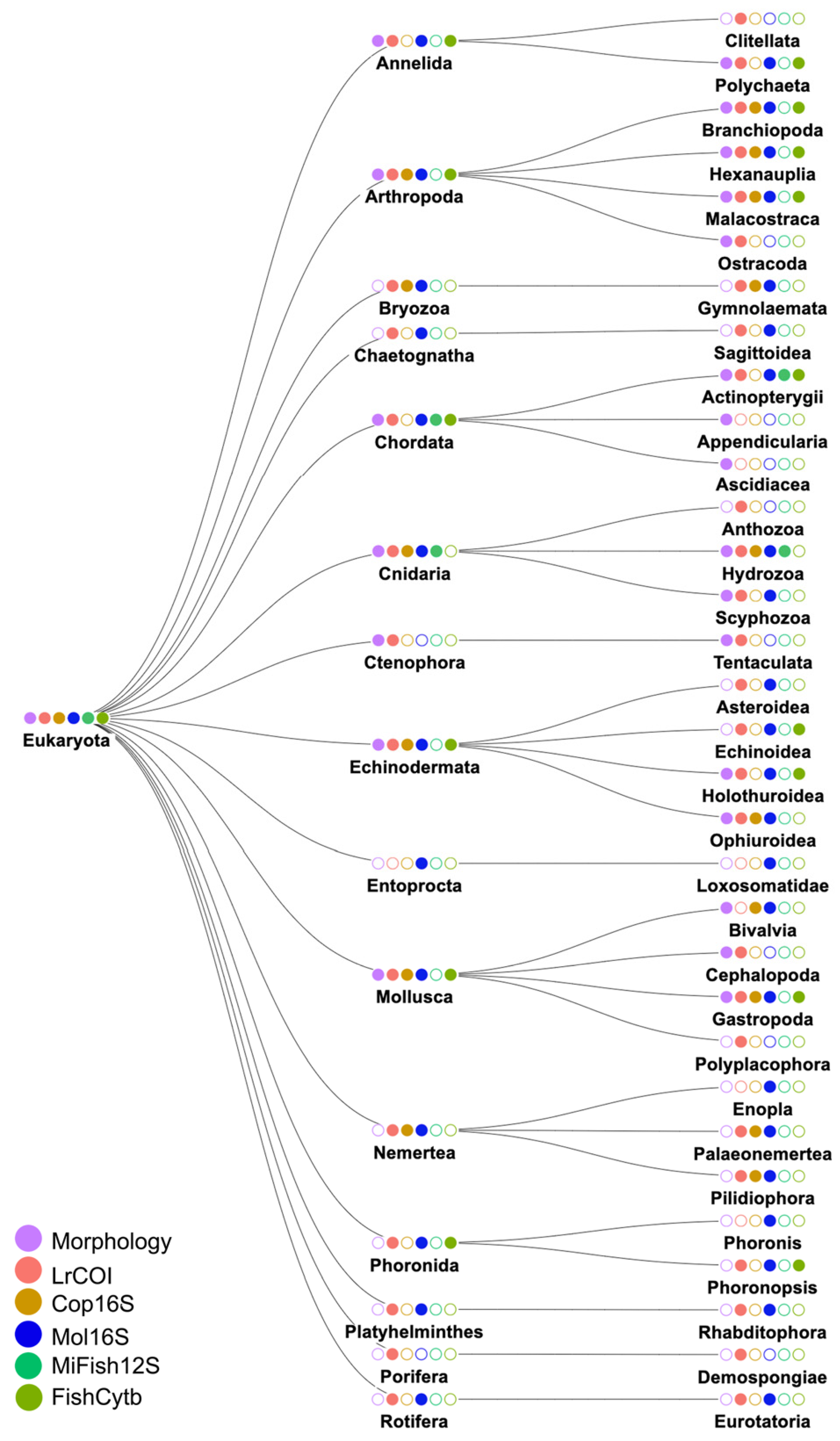
3.2. Species Identities and Distributions of Major Taxa

Major taxonomic groups resolved by the metabarcoding markers are detailed below by their invertebrate phylum (in alphabetical order), followed by fishes. We additionally relate these to morphology identifications (Figure 6, Supplementary Table S4).

3.2.1. Phylum Annelida: Class Polychaeta (Bristleworms, Fanworms, Clamworms) (Figure 6B, Supplementary Table S4)

The markers identified 26 species of polychaete annelids (mostly larvae), including 17 (65.4%) by LrCOI (of which six (35.3%) were unique) and 12 (46.2%) by Mol16S (eight (66.7%) were unique). Mol16S also delineated six others to the level of genus (including Diopatra). Five species identifications were shared by LrCOI and Mol16S, including Proceraea okadai, which is native to Asia and has invaded the Salish Sea (and San Francisco Bay) [70,98]. Mol16S and FishCytb identified another nonindigenous polychaete, Hediste diadroma, which likewise invaded the Salish Sea and San Francisco Bay from Japan [99]. FishCytb discerned two other polychaete species, with just one being unique: the red-banded commensal scale worm, Arctonoe vittata. In summary, the combination of LrCOI and Mol16S resolved most of the polychaete species, with none being identifiable by our morphology.

3.2.2. Phylum Arthropoda: Class Crustacea (Supplementary Table S4)

Crustaceans were variously identified morphologically and by four markers (LrCOI, Cop16S, Mol16S, and FishCytb), having the broadest coverage. Figure 4A shows 10 species—all are crustaceans—identified in common by morphology and the two general invertebrate markers (LrCOI, Mol16S): four in Order Copepoda, four in Order Decapoda, and two in Order Euphausiacea. With the metabarcoding markers alone, we additionally identified barnacles (Order Cirripedia) and water fleas (Order Cladocera) to species.
Order Cirripedia (barnacles): Seven barnacle species were discerned using LrCOI, four species by Cop16S (including a unique Rhizocephala—a taxon that parasitizes decapods), and five species (two were unique) with Mol16S; none were morphologically identified. Together, the markers were successful at identifying barnacle larvae.
Order Cladocera (water fleas): The brackish water species Pleopis polyphemoides was found by LrCOI, Cop16S, and Mol16S alike (the latter showed very high representation in autumn F). Evadne nordmanni was identified by both LrCOI and Mol16S, and E. spinifera by Cop16S and Mol16S. LrCOI identified three species, with the Arctic species Podon leuckartii being rare. Mol16S also identified three species; both Mol16S and LrCOI were needed to resolve the cladocerans.
Order Copepoda (copepods) (Figure 5, Figure 6C and Figure 7): Morphology identified many more copepod species than did our markers. The abundant cyclopoid copepods Ditrichocorycaeus anglicus and Oithona similis were solely found with morphology (see Discussion). LrCOI identified 15 calanoid copepod species, including two that otherwise were undetected. However, LrCOI did not discern the genus Neocalanus, including the species N. plumchrus, which was identified by morphology, Cop16S, and Mol16S.
Relationships between morphological carbon biomass and the proportion of copepod species sequence reads for two markers (LrCOI and Cop16S) are shown in Figure 7. Results varied widely by species and marker, with the highest correspondence being for Acartia longiremis with Cop16S (R2 = 0.90, r = 0.97); however, this was not significant with the stringent correction (Figure 7B). This species had similar prevalence in LrCOI and Cop16S (Supplementary Table S4), including in the spring and autumn seasons at site A (the closest location to the ocean) (Figure 6C). It also occurred in samples where it was morphologically undetected; those were likely early copepodite stages that could not be identified.
Calanus pacificus was prevalent and widespread in many samples (Figure 6C), whose morphological proportions and sequence abundances appeared similarly correlated for LrCOI and Cop16S (Figure 7). LrCOI read proportions and morphological prevalence also corresponded for Centropages abdominalis (Figure 7A), which was widespread in the spring (Figure 6B). Metridia pacifica was discerned by both LrCOI sequences and morphology in seven cases and by sequences alone in two others. Figure 7A shows the significant relationship between LrCOI sequence read proportions and carbon biomass. Pseudocalanus newmani was prevalent, whose sequence reads and morphology matched in most samples (Figure 6C and Figure 7A). In these examples, greater correspondence between the two data sets occurred when the species was abundant (Figure 7).
Cop16S identified just 10 copepod species, yet it was the sole marker to uncover two: Acartia tonsa (also in some morphological samples) and Racovitzanus antarcticus (site A). Read numbers for all markers were low or absent for Calanus marshallae, which also had low numbers and low biomass with morphology. The LrCOI and Cop16S markers thus appear complementary and were not entirely duplicative for copepods.
Order Decapoda (crabs, shrimps) (Figure 6D, Supplementary Figure S2A): LrCOI uncovered a broad diversity of decapods not identified by other markers or morphologically (Figure 5 and Figure 6D, Supplementary Figure S2A). Cancridae, an important commercial family in Puget Sound (which includes the Dungeness crab Metacarcinus magister), was captured by both LrCOI and morphology. Several morphological identifications of decapod larvae were restricted to the family or genus level, whereas metabarcoding identified them to species. LrCOI failed to identify three decapod species, which were all detected by both Mol16S and Cop16S. Mol16S uniquely identified the alpheid shrimp genus Betaeus at a site that lacked LrCOI data. Cop16S also identified three unique decapod species.
Order Euphausiacea (krills) (Figure 6D, Supplementary Figure S3): Four krill species were identified by four markers (LrCOI, Cop16S, Mol16S, and FishCytb), including North Pacific krill Euphausia pacifica (and also by morphology) and Arctic krill Thysanoessa raschii (and morphology). Thysanoessa spinifera was found with LrCOI (and morphology), and the northern species T. inermis was found by Cop16S and Mol16S. Occurrences of E. pacifica matched for LrCOI and morphology in nine samples, being very abundant; the species also had high Cop16S sequence reads at autumn site E in both vertical and oblique tows. Euphausia pacifica also showed high correspondence between sequence reads and biomass (Supplementary Figure S3).

3.2.3. Phylum Cnidaria (Supplementary Figure S2B, Supplementary Table S4)

We identified cnidarians belonging to: Class Hydrozoa (hydroids, colonial jellies, siphonophores), Class Anthozoa (sea anemones, corals, sea Fans), and Class Scyphozoa (true jelly fish). Cnidarians were primarily detected by morphology and LrCOI. Class Anthozoa was solely identified with LrCOI, as well as the Hydrozoa family Bougainvillidae. LrCOI identified 17 Hydrozoa species, with several uniquely found by it. LrCOI identified six species that were identifiable just at the family level with morphology and four other species that were morphologically identifiable solely at the genus level. Two key species that are abundant in Puget Sound, Aequorea victoria and Muggiaea atlantica, were identified to species by morphology alone (although LrCOI classified the latter to the genus level).
Mol16S detected two cnidarian species: the scyphozoan fried-egg jellyfish Phacellophora camtschatica (also identified by LrCOI) and the pink helmet hydrozoan Aglantha digitale (also identified by Cop16S and morphology, but not found by LrCOI). MiFish12S solely identified a single taxon (Melicertidae; Order Leptothecata), which is a thecate hydrozoan that appeared uniquely discerned by it.

3.2.4. Phylum Echinodermata (Supplementary Figure S2C, Supplementary Table S4)

We identified echinoderms belonging to Class Holothuroidea (sea cucumbers), Class Asteroidea (sea stars), Class Ophiuroidea (serpent and brittle stars), and Class Echinoidea (sea urchins and cake urchins). Echinoderm larvae were well-resolved by both LrCOI and Mol16S, which together identified 18 species. Morphology identified none to species, with holothurians and ophiuroids limited to the class level and echinoids and asteroids grouped together in the phylum. LrCOI identified 12 species, with six appearing unique to that marker. Mol16S also delineated 12 species, of which six solely were found by it; however, three occurred in samples lacking LrCOI data. Mol16S solely detected the giant pink sea star Pisaster brevispinus. The orange sea cucumber Cucumaria miniate was the most widespread species among sites (in spring), identified by LrCOI and Mol16S.

3.2.5. Phylum Mollusca (Supplementary Table S4)

Class Bivalvia (clams, mussels, scallops, and allies) (Supplementary Table S4): All of the bivalve larvae were resolved by Mol16S, which identified seven species and one genus (Modiolus); all occurred in autumn. Native species included the thin-shelled littleneck clam Callithaca tenerrima, the edible basket of heart cockle Clinocardium nuttallii that is being targeted for aquaculture, the corrugated clam Humilaria kennerleyi, the Pacific blue mussel Mytilus trossulus, and Xylophaga washingtona (the sole species also found by Cop16S).
Class Gastropoda (snails, limpets, pteropods, nudibranchs, and sea slugs) (Supplementary Figure S2D, Supplementary Table S4): Gastropods were resolved by the markers LrCOI, Cop16S, and Mol16S, and a few were identified by morphology. Morphology solely identified the periwinkle snail genus Littorina and two pteropods—the sea angel Clione limacina and the sea butterfly Limacina helicina. The winged sea slug Gastropteron pacificum was found both by morphology and LrCOI.
Mol16S identified 29 (70.1%) of the 41 gastropod species found by the markers, with 23 (79%) being unique and three others to the genus level. However, 17 of those 23 species (74%) exclusively occurred in sites lacking LrCOI and/or Cop16S data. LrCOI identified 13 (31.7%) gastropod species, nine (69%) by itself; some sites were also surveyed with Mol16S but did not resolve those species. Just one species was identified by LrCOI and Mol16S in common; two species were identified by LrCOI, Cop16S, and Mol16S alike. Cop16S found just five of the species; all matched those from Mol16S. However, many of the unique LrCOI and Mol16S species occurred in samples that were missing Cop16S results, so that marker’s scope may be broader than indicated here. Mol16S was best at identifying the gastropod larvae, but supplementation with LrCOI and morphology was needed for fuller coverage.

3.2.6. Phylum Chordata: Class Osteichthyes (bony fishes) (Figure 6E, Supplementary Figure S2E)

Metabarcoding identified 39 fish species belonging to 20 families in the Order Actinopterygii (ray-finned fishes). Our zooplankton morphology identified fish just to class (note that we did not consult a fish larvae expert). Four fish species were identified jointly by four markers (LrCOI, Mol16S, MiFish12S, and FishCytb): North Pacific hake Merluccius productus (Family Merlucciidae), Pacific staghorn sculpin Lepidocottus armatus (Cottidae), walleye pollock Gadus chalcogrammus (Gadiidae), and Pacific herring Clupea pallasii (Clupeidae). MiFish12S identified pollock to just the genus level, from sites where the other markers identified it to species.
Our FishCytb marker identified the most fish species, with seven being uniquely detected, including the nonindigenous American shad Alosa sapidissima (Clupeidae) (see Discussion). Many Pleuronectidae flatfish species were uniquely identified by FishCytb (mostly larvae in spring, and many at site E). MiFish12S identified 20 fish species, of which three were exclusively found by it. LrCOI denoted 17 species, three by itself. Mol16S identified 17 species, three by itself.
Two fish species—Black Sea sprat Clupeonella cultriventris and Eurasian ruffe Gymnocephalus cernua—might have been due to contamination stemming from a former student’s work, who amplified their extracted DNA to test the fish assays (Supplementary Table S5) [100]. Although they did not amplify in our negative controls, sprat and ruffe appear unlikely to be present in the Salish Sea; thus, those samples (as well as the others) are being redone in an independent lab (MCIC, including all extractions and amplifications) for the multi-year analyses. We thus limit our present discussion to species that have highest confidence (see Supplementary Tables S5 and S6).

4. Discussion

4.1. Metabarcoding Marker Specificities

The metabarcoding markers that we evaluated each possess different taxonomic resolutions and strengths, for which identifications to species are the most valuable for understanding the compositions of biological communities and interpreting their dynamics. Relatively few species (eight) were identified in common by our morphological analysis and the three invertebrate metabarcoding markers (Figure 4B); however, many were uniquely identified by the different markers (i.e., 97 species by LrCOI, 92 by Mol16S, and five by Cop16S) or by morphology (25 species). This points to the utility of employing multiple metabarcoding markers to address broadscale species diversity across multiple taxa and for ground-truthing with morphological identifications in designing and conducting studies.
In our analysis, LrCOI was best overall at resolving crustacean species, including copepods, barnacles, cladocerans, shrimps, crabs, and krills. LrCOI also identified hydrozoan cnidarians, polychaete annelids, echinoderms, and some fishes. Like our findings, Ershova et al. (2021) [101] discerned that their COI marker yielded fewer copepod reads and missed several copepod taxa (e.g., Acartia, Metridia, Microsetella) that were discerned with morphology. Our LrCOI marker likewise did not resolve some copepod taxa, notably cyclopoids, as was also noted by Matthews et al. (2021) [102]. For our cyclopoid copepods, primer mismatches and their relatively small sizes (and consequently, less DNA) likely contributed to their lack of representation. However, why Ditrichocoryceaus anglicus was not detected when it occurred in high biomass and has a reference barcode is not clear, meriting additional investigation.
Casey et al. (2020) [51] employed the same LrCOI marker that we did, analyzing tropical coral reef taxa in comparison to their nuclear 18S RNA sequences. They found that LrCOI resolved Bryozoa and Porifera (sponges) better than their nuclear 18S marker; however, their study focused on higher taxonomic levels. Likewise, none of our markers identified sponges to genus or species, but Mol16S identified one bryozoan to species and three others at higher levels. Both of their markers detected some fishes [51], as did our LrCOI marker.
The Mol16S marker’s strengths were in elucidating a wide variety of mollusk species, including gastropod snails, nudibranch larvae, and bivalves, which could not be identified by morphology. It also identified a broad realm of echinoderm and polychaete larvae to species (which also could not be identified with morphology), as well as a variety of crustacean species (including cladocerans, barnacles, and decapods). Mol16S also identified a bryozoan species, a rotifer, a phoronid horseshoe worm species, an enteropneust hemichordate species, and 17 fish species, with three fish species uniquely found by the marker. Its resolution of fishes differed with and without the fish blocker primer (see Figure 4B and [36]). Although this marker was originally designed for freshwater mollusks [36], it displays broad utility for identifying marine mollusk species, as well as resolving a variety of other marine invertebrates.
Our metabarcoding identified many types of zooplankton that were missed by our morphology; most of these belonged to Bryozoa, Chaetognatha, Nemertea, Phoronida, Platyhelminthes, Porifera, and Rotifera. Metabarcoding results were especially adept at identifying polychaete, cnidarian, barnacle, decapod, gastropod, bivalve, echinoderm, and early life stage fishes to species, hallmarking their usefulness for analyzing zooplankton community composition and structure.
Fish species were best resolved by the combination of the MiFish12S and the FishCytb markers, since the taxa identified by each did not entirely overlap. FishCytb was especially effective at identifying Pleuronectidae flatfish species, some of which were not discerned by MiFish12S (e.g., English sole Parophrys vetulus, starry flounder Platichthys stellatus, butter sole Isopsetta isolepis, Pacific rock sole Lepidopsetta bilineata, and Pacific sand sole Psettichthys melanostictus), despite their prevalence and sequence abundances. A longer fish-specific targeted metabarcoding marker region (“FishU”, averaging 373 bp) designed by Kim et al. (2021) that spans between the 12S and 16S RNA genes likewise resolved species of Pleuronectidae that were missed by MiFish12S in their ichthyoplankton study in the east Japan Sea [37]. Longer markers, such as FishU, can provide more sequence characters to aid species identification and discern among closely related ones [37], provided that the reference sequences are available. Targeted taxon-specific markers also avoid extraneous sequence reads for other non-targeted taxa [36,37,103].
Future analyses for all markers are anticipated to improve in resolution as more species are sequenced and referenced in NCBI [86] and other sequence data repositories.

4.2. Species Detected by Morphology and Missed by Metabarcoding

A few taxa were abundant in our morphology dataset but were not identified with metabarcoding, often due to poor representation in the NCBI reference database [85]. Notably, cyclopoid copepods were missed by metabarcoding, including the abundant species Ditrichocorycaeus anglicus (up to 15.3% of the biomass). This species was well-represented in NCBI, and the LrCOI forward primer contained just one mismatch, but it was not detected with any of the metabarcoding markers; this discrepancy is being further investigated in follow-up work. Cyclopoid copepods in the genus Oithona were also abundant in the morphology counts (up to 9.43% of the individuals), leading to the expectation that they should be detectable with metabarcoding. However, their small individual sizes led to their proportionally small biomass representation (average 0.1%, with a maximum of 0.7%), which, combined with PCR bias (1–3 mismatches in the forward LrCOI primer), might have resulted in a lack of metabarcoding detections. Appendicularians belonging to the genus Oikopleura were also missed by metabarcoding, potentially due to a lack of reference sequences for the species most likely to occur in the Salish Sea. Additionally, the abundant amphipod Cyphocaris challengeri lacked species representation in the NCBI at the time of analysis, leading to its non-detection [95].

4.3. Sequence Read Proportion Relationships and Potential Biases

Many other investigations that compared the relative proportions of sequence reads from metabarcoding assays to specimen counts and/or biomass estimates from morphological identifications have found positive correlations [61,101,102,103,104,105,106], whereas some have not [107,108]. For example, Matthews et al. (2021) [102] described a positive relationship between metabarcode read counts and relative abundance as well as biomass for copepods using LrCOI, as was the overall pattern in our study. Also like our results, Ershova et al. (2021) [101] discerned a positive correlation of their COI marker with biomass estimates for copepods and a variety of other invertebrates. Examining multiple examples and factors, an overview by Lamb et al. (2019) [109] concluded a positive yet weak correlation between sequence reads and numbers of individuals per species across metabarcoding studies, which averaged R = 0.52 ± 0.34. Their range [109] corresponded to the correlation values we obtained for copepods. We similarly found that our results were quite variable among different taxa using LrCOI, for which three crustaceans (of 12) had significant corrected p-values (Calanus pacificus, Metridia pacifica, and Euphausia pacifica). Lamb et al. (2019) [109] discerned that weaker relationships occurred when species varied greatly in body sizes. In our results, the correlation between relative abundance and biomass increased when analyses were restricted to just the Copepoda as opposed to using the entire dataset, suggesting that including taxa of vastly different biomass can skew the results.
In our results, the species with the greatest ranges in biomass among sampled individuals showed significant correlations. This finding makes sense given an average four-fold potential shift in relative abundance predicted from PCR bias alone in models by Shelton et al. (2023) [110]. Correlations for some of our most abundant copepods (Centropages abdominalis, Acartia longiremis) had positive values, yet were insignificant here (with the stringent correction employed). These trends merit caution in interpretation, especially with the small sample sizes used in the present pilot study, pending our further multi-year analyses.
Multiple factors can lead to differences between true biomass estimates and read count data, including those prior to amplification (e.g., mt copy number, DNA extraction efficiency, sampling stochasticity, sample preservation) and others that influence the PCR reaction itself (e.g., PCR biases resulting from primer mismatch, inhibition, and other non-primer-mismatch sources leading to differences in amplification efficiency) [109,110,111,112,113,114,115,116]. For example, a meta-analysis by Piñol et al. (2015) [113] found that primer mismatches accounted for 75% of amplification variation in studies. Strategies have been proposed to address amplification biases, aiming to employ a mechanistic framework for quantitative metabarcoding data [110,114,115,116]. Those approaches require additional/modified sequencing protocols, which further studies should consider adopting. Our findings highlight the need to adopt protocol adaptations [110,114,115,116,117] that facilitate quantitative comparisons of sequence proportions with biomass.

4.4. Threatened or Vulnerable Fishery Species

The present approach provides an important example of how metabarcoding with multiple markers may be used to determine the species compositions of zooplankton and ichthyoplankton, including rare, threatened, and vulnerable species. Notably, metabarcoding analyses of ichthyoplankton in other marine ecosystems have shown improved accuracy for species identification in ecological assessments [117,118,119,120].
Chum salmon Oncorhynchus keta was found in our autumn E and F samples; the summer spawning run in Hood Canal (site F) comprises an ESU (evolutionary significant unit), which (since 1992) has been federally listed as threatened under the U.S. 1972 Endangered Species Act [121]. The Washington Department of Fish and Wildlife regards the chum salmon in Puget Sound as having moderate to high vulnerability to climate change [122], which suggests data such as ours may provide monitoring value.
The Washington Department of Fish and Wildlife also notes that the southern Puget Sound population of walleye pollock Gadus chalcogrammus is relatively isolated from other populations, located at the southern end of the species’ range, and has moderate vulnerability to climate change [123]. We identified this species at all of our sites in the spring, indicating widespread occurrence. Its recreational harvest within Puget Sound is closed, with the exception of restricted fishing in the San Juan Islands and Strait of Juan de Fuca [123], rendering its population data of interest.
The Pacific herring, Clupea pallasi, an important forage fish, was also very abundant and widespread across our spring and autumn sites (found with both fish markers). A genetic study by Small et al. (2002) discerned that Pacific herring varied significantly across Puget Sound [124]. However, its variation has not been regarded as meriting federal listing under the ESA [125]. Yet, Pacific herring is currently identified as a “Species of Greatest Conservation Need (SGCN)” under the Washington State Wildlife Action Plan (SWAP) [126], for which monitoring with metabarcoding may reveal further patterns.
Metabarcoding found Pacific hake Merluccius productus larvae to be relatively abundant in our spring samples. The Puget Sound population has been described to genetically vary from the large coastal population [127] and has undergone significant reductions in numbers [15]. Additionally, a study of otolith growth patterns by Chittaro et al. (2022) indicated that the Puget Sound population has significantly declined in somatic growth rate and body size over the past five decades [128]. Thus, monitoring its larval population patterns, along with those of other species of fishery and conservation interest, may provide an important application for ichthyoplankton metabarcoding.
Knowledge of adult and larval fish distributional patterns is important for assessing their population- and community-level responses to ongoing environmental fluctuations and changes. Elucidating these relationships using metabarcoding, along with targeted population genetic analyses, should provide important information for evaluating the trends of Salish Sea species in the future.

4.5. Non-Indigenous Species Detections

The present investigation identified possible nonindigenous species whose larval distributions can be assessed with metabarcoding. We evaluated the quality of the taxonomic assignment to each of these species (Methods and Supplementary Table S6), since invasions can have implications for management responses [9,93]. We assessed nine putative nonindigenous marine/estuarine species, of which four were regarded as having high confidence due to percent identity matches to the sequence reference database and our other criteria (Supplementary Table S6). The remainder are excluded from discussion here due to lower percent identity matches and/or missing reference sequences for potential closely related local species, pending our further analyses of the complete multi-year data set (see Supplementary Table S6). Notably, high confidence values support two nonindigenous polychaetes found by the LrCOI marker: Proceraea okadai and Hediste diadroma, which both have known introductions to the Salish Sea (and San Francisco Bay) from Asia [70,98,99].
The shad, Alosa sapidissima, was another confident nonindigenous species match. It is native to the northwestern Atlantic Ocean region, was intentionally introduced to the San Francisco Bay watershed in 1871 [129], and then was collected in the Columbia River in 1876 [130]. We detected shad larvae at site D in the spring. Adults and juveniles are reported to be common in Skagit Bay (near our site B, where we did not find them) and rare in other parts of Puget Sound [130]. The shad is anadromous and briefly enters freshwater to spawn, after which most adults die. Shad can significantly alter the zooplankton community by consuming large numbers [131], rendering metabarcoding results potentially important for ecological monitoring of zooplankton diversity patterns.
Assignment of the invasive Eurasian zebra mussel Dreissena polymorpha appeared to merit confidence according to our criteria (it was detected at the spring D location and autumn at B, C, and E) (Supplementary Table S6). However, since it was previously worked on in the laboratory, this could be contamination (Supplementary Table S5), which is being further evaluated. The zebra mussel is a very deleterious and prolific fouling species that has become widely distributed throughout much of North American fresh and estuarine waters after its initial establishment in the Great Lakes from multiple Ponto-Caspian source populations (summarized by [58]). The zebra mussel has not been reported yet from the Salish Sea but occurs in many other western U.S. locations; it was also recently discovered living in imported moss ball algae for sale in aquariums and pet stores in Seattle, Washington, as well as in 20 other states [58]. Its possible occurrence is being further tested in our multi-year Salish Sea study, whose DNA extraction and laboratory steps were all done at Ohio State University’s Molecular and Cellular Imaging Facility (https://mcic.osu.edu/home, accessed on 12 November 2023) to circumvent contamination.
We did not discern the invasive European green crab Carcinus maenas in our study, despite the high-resolution capacity of our LrCOI and Mol16S markers and our morphology for decapod crustaceans. Although the green crab was then being collected from the outer Washington coast, it had not yet become well-established in these Salish Sea sites by our 2018 sampling. The European green crab was first documented in the Salish Sea at Sooke Basin, British Columbia in 2012, in the San Juan Islands and Padilla Bay in 2016 [132,133], and in the Hood Canal in 2022 (after our sampling) [134]. Moreover, its numbers remained low across most of the Salish Sea until after our study [134]. Sampling outside of the Salish Sea on the outer coast of Vancouver Island, British Columbia, in 2017 by Westfall et al. (2022) [135] found very low numbers of the species in trap collections and little traces in water eDNA samples using quantitative (q)PCR, and no DNA was detected in the analysis of zooplankton net tows; the latter appears similar to our Salish Sea sampling results. This species is being further evaluated in our multi-year comparisons.
Metabarcoding data, such as ours, provide valuable knowledge about nonindigenous species occurrences, distributions, and life histories. For example, Fernández-Álvarez and Machordom (2013) [136] identified a cryptic nemertean invasion in the Mediterranean Sea using conventional single-individual barcoding of COI, whose distributional range and distinction from other species would likely also be discernable with metabarcoding. Here we found several putative nonindigenous species with our markers, some of which may be new documentation in the Salish Sea; these merit further verification and sampling surveillance. There is a pronounced need for reference specimens, accompanied by mapped sites and metadata documentation, along with diagnostic DNA sequences, following recommendations summarized by the National Invasive Species Council Task Force in Morisette et al. (2021) [94]. The Early Detection and Rapid Response (EDRR) program for invasive species by the US Geological Survey aims to provide such documentation [137].

4.6. Species Identifications and Reference Libraries

Correct species identifications are vitally important for valid ecological comparisons, yet they are often overlooked. Notably, Bianchi and Gonçalves (2021) [138] pointed out that misidentifications and problematic taxonomic metadata are a recurrent issue significantly affecting sequence reference databases, including the Global Biodiversity Information Facility (GBIF), the Barcode of Life Data System (BOLD), and NCBI GenBank. Misspellings and invalid names sometimes exceed 10% of deposited sequences for a given species, along with poor-quality sequences [139]. Such mistakes compromise the integrity of reference databases and appear to affect many studies (see [9,43,52,112,138,139,140,141,142,143,144,145]).
Here we found limitations due to the number of species that lacked diagnostic sequence data in reference databases at the time of our study (see Figure 6A,F). Around the world, there is a growing effort to combat this lack of reference sequences with the increasing cost-effectiveness of whole mitogenome and whole genome sequencing efforts. Such efforts include a collaboration being undertaken for all U.S. marine fishes by NOAA Fisheries, Smithsonian’s National Museum of Natural History, and other federal partners (e.g., [140,141]), for zooplankton with the MetaZooGene collaboration by the Scientific Committee on Oceanic Research of the International Science Council [142], and for all marine species with a US Oceans Biocode (Meyer et al. 2021 [143]). Reference sequence data that are accompanied by specimens, their collection data, and preserved tissue samples in museum repositories are especially valuable (see [138,139,140,141,142,143,144,145]).
In the future, metabarcoding data sets like ours can be used to identify species from the original sequences that once were not diagnosable, by making new queries of improved and augmented reference sequence databases. Additionally, longer sequence reads will allow greater accuracy in identifications (see [37]), which are currently hampered by the limitations in sequence read lengths with most existing HTS platforms [140,141,142,143]. As shown by our investigation, the use of multiple gene regions and multiple markers can significantly enhance taxonomic coverage, confidence, and reliability for present-day metabarcoding efforts.

4.7. Ecological Patterns and Trends

Species that are congruently identified by more than one metabarcoding marker and gene region provide strong verification of their presence in field-collected samples [42,52]. For rare and poorly known taxa, especially at their early life stages, metabarcoding identifications are very valuable—provided that the sequence reference databases exist and are correct [138,139,140,141,142,143,144,145].
The larval macroinvertebrates and fish assayed in this project are the key to adult recruitment for the abundant fisheries of the Salish Sea and much of the NE Pacific Coast. It is these early life history stages that are under the most intense selection and are the most ephemeral and vulnerable (see [146]). For example, it is hypothesized that warming and other anthropogenic factors may alter the timing of phytoplankton blooms and their reliant zooplankton populations; this may put larval communities out of synchrony with their prey [12,13,16]. Species identifications of these stages with metabarcoding pave the way towards important biomonitoring for the future. Whereas many metabarcoding efforts to date have focused on taxa identified only at higher levels using less variable marker sequence regions, we argue that this limits ecological studies to generalities and that identifications of species are essential. Metabarcoding offers the opportunity to identify exactly what species of larvae are in the plankton when and in which habitats, in cases where morphology cannot distinguish among them [9,10,11]. We thus envision that future monitoring with these markers and others will provide important data on these patterns in relation to environmental conditions.
Seasonal differences between spring and autumn were apparent in the species compositions of the zooplankton and ichthyoplankton communities with our metabarcoding and morphological results alike; similar seasonal community trends have characterized other metabarcoding studies [30]. The patterns found here correspond to expected reproductive seasons, as well as with the species’ described geographic distributions and habitats [15,66]. For example, our metabarcoding detected spatial patterns in copepod species related to oceanic conditions (i.e., distance of the site from the ocean), such as the elevated representation of A. longiremis and C. marshallae at site A (more oceanic), agreeing with their morphological occurrences [66]. Site A also had a more distinct fish species composition, including the slipskin snailfish Liparis fucensis, corresponding to known biogeographic distributions [15]. Metabarcoding thus holds considerable promise for resolving both species compositions and timings of larvae in the plankton, which otherwise are difficult to resolve.
The use of metabarcoding to understand zooplankton and ichthyoplankton communities is expanding, including investigations of diversity patterns across: vertical gradients in the mesopelagic zone [147], seasons in the Red Sea [148], currents and water masses in the Pacific versus the Atlantic [149], and trophic levels in the Kuroshio region of Japan [150]. The metabarcoding markers used here demonstrate success in resolving a wide realm of invertebrate and fish taxa, pointing to a broad application for understanding planktonic community ecology at the species level, which is not achievable by traditional taxonomy. Metabarcoding is particularly applicable for resolving species compositions of plankton, which contain larval stages that lack morphological features to distinguish among them but can be readily identified with DNA sequences.

5. Conclusions

This multi-gene metabarcoding marker approach holds considerable promise to advance scientific ability for assessing species identities and compositions of planktonic communities, as well as to evaluate their responses to environmental conditions. Moreover, the approach is powerful and data-rich, yielding results that are readily integrated into existing ecological sampling and modeling efforts. Currently, there are species identification issues stemming from a lack of available reference sequences, along with museum voucher specimens, preserved tissues, and DNA samples for comparisons; sequence databases are also fraught with incorrect, erroneous scientific names and incorrect systematic classifications [9,43,52,112,136,137,138,139,140,141,142,143,144,145]. Additionally, requiring multiple markers for assessment significantly increases the cost of such analysis. However, coupling targeted (taxon-specific) with more general metabarcoding markers, as accomplished here, offers the resolution power for discerning both known and unknown species. For example, McCarthy et al. (2022) [117] found that a highly targeted metabarcoding marker designed for a single species and sequenced at great depth had a lower limit level of detection than did qPCR; thus, by coupling multiple metabarcoding markers, one can answer many questions in a single ecological study.
Metabarcoding with multiple markers shows significant aptitude to aid in the elucidation of patterns and changes in zooplankton communities towards understanding their responses to chemical and physical alterations and interpreting species diversity. This is best accomplished with careful reference to companion morphological analyses, which are also needed to provide abundance and biomass information. Laboratory testing with mock communities that contain DNA for the range of targeted taxa/species can be used to compare resolution among metabarcoding markers alongside unknown taxa from the field (see [36,37,62,103]). Our overall project outcomes here are projected to help resolve species-level knowledge of the variability and consistency of the zooplanktonic communities over time and space. As steps and procedures increasingly become automated with biotechnology and in situ instrumentation, elucidating zooplankton communities in near real-time will greatly advance ecological understanding of their responses to changing environmental conditions.

Supplementary Materials

The following supporting information can be downloaded at: https://www.mdpi.com/article/10.3390/dna4010001/s1, Table S1. Metabarcoding markers and gene regions, references, primer sequences approximate target sequence length, and PCR parameters; Table S2. Total number of reads (pairs and single reads post-merge) at each step in the quality control pipeline; Table S3. Amplicon sequence variant (ASV) counts for each metabarcoding marker; Table S4. Master dataset from Salish Sea metabarcoding and morphological analysis; Table S5. Species studied in the laboratory and whether or not they were detected in this metabarcoding study; Table S6. Assessment of assigned sequence variants (ASVs) to putative nonindigenous species; Figure S1. Taxonomic and read count/relative abundance information viewed through Krona plot hierarchical data browsers. doi:10.6084/m9.figshare.21791738; Figure S2A. Decapoda Crustacea species resolved by morphology and/or four metabarcoding markers; Figure S2B. Cnidaria species resolved by morphology and/or four metabarcoding markers; Figure S2C. Echinodermata species resolved by morphology and/or three invertebrate metabarcoding markers; Figure S2D. Gastropoda Mollusca species resolved by morphology and/or three metabarcoding markers; Figure S2E. Actinopterygii (Teleostei) fish species resolved by morphology and/or four metabarcoding markers; Figure S3. Proportion of Arthropoda species carbon biomass versus proportion of sequence reads (ASVs merged per species) from metabarcoding marker LrCOI.

Author Contributions

Conceptualization, C.A.S. and J.E.K.; methodology, C.A.S., J.E.K., S.M.M., H.K.S. and E.L.N.; software, S.M.M. and H.K.S.; validation, S.M.M. and H.K.S.; formal analysis, S.M.M. and H.K.S.; investigation, E.L.N.; resources, J.E.K. and C.A.S.; data curation, S.M.M.; writing—original draft preparation, C.A.S.; writing—review and editing, C.A.S., J.E.K., S.M.M., H.K.S. and E.L.N.; visualization, S.M.M. and H.K.S.; supervision, J.E.K. and C.A.S.; project administration, J.E.K. and C.A.S.; funding acquisition, J.E.K. and C.A.S. All authors have read and agreed to the published version of the manuscript.

Funding

This research was funded by the Washington Sea Grant Program A18OAR417009, “Metagenomic fluctuations of zooplankton and ichthyoplankton communities in the Salish Sea: association with water chemistry”, to J.E.K. and C.A.S.; S.M.M. was also partially supported through the Joint Cooperative Institute for Climate, Ocean, and Ecosystem Studies under the NOAA Cooperative Agreement NA15OAR4320063, with funding awarded to CAS as the principal investigator.

Institutional Review Board Statement

Not applicable.

Data Availability Statement

Sequencing read data are available publicly through the National Center for Biotechnology Information (NCBI) Sequence Read Archive (SRA), under project accession PRJNA915814. Supplementary Materials (figures, tables, and datasets) for the morphological and metabarcoding marker data and results, including analysis products, are archived on figshare at https://figshare.com/projects/Supplementary_Material_for_Evaluating_mtDNA_metabarcoding_markers_to_identify_zooplankton_and_ichthyoplankton_in_the_Salish_Sea_Resolution_in_comparison_to_morphology_/156479. The custom script used for taxonomic identification by SMM is accessible on GitHub at https://github.com/McAllister-NOAA/asv_to_taxonomy (accessed on 12 November 2023).

Acknowledgments

We extend our thanks and great appreciation to Russell Callender and the Washington Sea Grant Program team for their understanding and help, especially during project delays and personnel issues during the COVID-19 pandemic. We greatly appreciate collection help from Jan Newton, Terrie Klinger, Amanda Winans, Amy Wyeth, Anna McLaskey, and Beth Curry and the Washington Ocean Acidification program and research cruises. Morphological identifications were conducted by BethElLee Herrmann, Olga Kalata, and Amanda Winans in the laboratory of JEK. Some genetics laboratory work was variously aided by members of the Genetics and Genomics Group at NOAA Pacific Marine Environmental Laboratory under the scientific direction of CAS, including Anna E. Elz, Kimberly Andrews, Matthew R. Snyder, Elizabeth Slikas, Nathaniel T. Marshall, and Matthew Galaska. We thank Thomas Ackerman, Frederick Averick, John Horne, and David Butterfield at the University of Washington’s Cooperative Institute (CICOES) for help with logistics and grant management. In addition, valuable information was provided about ocean acidification conditions in the Salish Sea by Richard A. Feely and about species’ presence and distributions by Meggen S. Chadsey, Matthew E. Neilson, Theodore Pietsch, James W. Orr, and Timothy Wood. The manuscript benefited from suggestions by NOAA reviewers Kelly D. Goodwin, Zachary Gold, and Allen Collins, and Smithsonian National Museum of Natural History colleagues Katherine Bemis, Katherine Murphy, and Chris Meyer. This is contribution #2022-1248 from the University of Washington CICOES and contribution #5460 from the NOAA Pacific Marine Environmental Laboratory (PMEL).

Conflicts of Interest

The authors declare no conflicts of interest.

References

  1. Coyle, K.O.; Pinchuk, A.K.; Eisner, L.B.; Napp, J.M. Zooplankton species composition, abundance and biomass on the eastern Bering Sea shelf during summer: The potential role of water-column stability and nutrients in structuring the zooplankton community. Deep. Sea Res. Part II 2008, 55, 1755–1791. [Google Scholar] [CrossRef]
  2. Pomerleau, C.; Sastri, A.R.; Beisner, B.E. Evaluation of functional trait diversity for marine zooplankton communities in the Northeast subarctic Pacific Ocean. J. Plankton Res. 2015, 37, 726. [Google Scholar] [CrossRef]
  3. Hirai, J.; Katakura, S.; Kasai, H.; Nagai, S. Cryptic zooplankton diversity revealed by a metagenetic approach to monitoring metazoan communities in the coastal waters of the Okhotsk Sea, Northeastern Hokkaido. Front. Mar. Sci. 2017, 4, 379. [Google Scholar] [CrossRef]
  4. Gobler, C.J.; Baumann, H. Hypoxia and acidification in ocean ecosystems: Coupled dynamics and effects on marine life. Biol. Lett. 2016, 5, 20150976. [Google Scholar] [CrossRef] [PubMed]
  5. Breitburg, D. Effects of hypoxia, and the balance between hypoxia and enrichment, on coastal fishes and fisheries. Estuaries 2002, 25, 767–781. [Google Scholar] [CrossRef]
  6. Keil, K.E.; Klinger, T.; Keister, J.E.; McLaskey, A.K. Comparative sensitivities of zooplankton to ocean acidification conditions in experimental and natural settings. Front. Mar. Sci. 2021, 86, 613778. [Google Scholar] [CrossRef]
  7. Yasuhara, M.; Hunt, G.; Dowsett, H.J.; Robinson, M.M.; Stoll, D.K. Latitudinal species diversity gradient of marine zooplankton for the last three million years. Ecol. Lett. 2012, 15, 1174–1179. [Google Scholar] [CrossRef]
  8. Patti, B.; Marco, T.; Angela, C. Interannual summer biodiversity changes in ichthyoplankton assemblages of the Strait of Sicily (Central Mediterranean) over the period 2001–2016. Front. Mar. Sci. 2022, 9, 960929. [Google Scholar] [CrossRef]
  9. Trebitz, A.S.; Hoffman, J.C.; Darling, J.A.; Pilgrim, E.M.; Kelly, J.R.; Brown, E.A.; Chadderton, W.L.; Egan, S.P.; Grey, E.K.; Hashsham, S.A.; et al. Early detection monitoring for aquatic non-indigenous species: Optimizing surveillance, incorporating advanced technologies, and identifying research needs. J. Environ. Manag. 2017, 202, 299–310. [Google Scholar] [CrossRef]
  10. Trebitz, A.S.; Hoffman, J.C.; Darling, J.A.; Pilgrim, E.M.; Kelly, J.R.; Brown, E.A.; Chadderton, W.L.; Egan, S.P.; Grey, E.K.; Hashsham, S.A.; et al. Diversity and distribution of meroplanktonic larvae in the Pacific Arctic and connectivity with adult benthic invertebrate communities. Front. Mar. Sci. 2019, 6, 490. [Google Scholar] [CrossRef]
  11. Ratcliffe, F.C.; Uren Webster, T.M.; Rodriguez-Barreto, D.; O’Rorke, R.; Garcia de Leaniz, C.; Consuegra, S. Quantitative assessment of fish larvae community composition in spawning areas using metabarcoding of bulk samples. Ecol. Appl. 2021, 31, e02284. [Google Scholar] [CrossRef] [PubMed]
  12. Canonico, G.; Buttigieg, P.L.; Montes, E.; Muller-Karger, F.E.; Stepien, C.; Wright, D.; Benson, A.; Helmuth, B.; Costello, M.; Sousa-Pinto, I.; et al. Global observational needs and resources for marine biodiversity. Front. Mar. Sci. 2019, 6, 367. [Google Scholar] [CrossRef]
  13. Bucklin, A.; Batta-Lona, P.G.; Questel, J.M.; Wiebe, P.H.; Richardson, D.E.; Copley, N.J.; Benson, A.L.; Helmuth, B.; Costello, M.; Sousa-Pinto, I.; et al. COI metabarcoding of zooplankton species diversity for time-series monitoring of the NW Atlantic continental shelf. Front. Mar. Sci. 2022, 9, 367. [Google Scholar] [CrossRef]
  14. Shu, L.; Ludwig, A.; Peng, Z. Standards for methods utilizing environmental DNA for detection of fish species: Review. Genes 2020, 11, 296. [Google Scholar] [CrossRef]
  15. Pietsch, T.; Orr, J.W. Fishes of the Salish Sea: Puget Sound and the Straits of Georgia and Juan de Fuca; University of Washington Press: Seattle, WA, USA, 2019; p. 1074. ISBN 9780295743745. [Google Scholar]
  16. Keister, J.E.; Winans, A.K.; Herrmann, B. Zooplankton community response to seasonal hypoxia: A test of three hypotheses. Diversity 2020, 12, 21. [Google Scholar] [CrossRef]
  17. Caldeira, K.; Wickett, M.E. Anthropogenic carbon and ocean pH. Nature 2003, 425, 365. [Google Scholar] [CrossRef] [PubMed]
  18. Barton, A.; Hales, B.; Waldbusser, G.C.; Langdon, C.; Feely, R.A. The Pacific oyster, Crassostrea gigas, shows negative correlation to naturally elevated carbon dioxide levels: Implications for near-term ocean acidification effects. Limnol. Oceanogr. 2012, 57, 698–710. [Google Scholar] [CrossRef]
  19. Feely, R.A.; Doney, S.C.; Cooley, S.R. Ocean acidification: Present conditions and future changes in a high-CO2 world. Oceanography 2009, 22, 36–47. [Google Scholar] [CrossRef]
  20. Feely, R.A.; Alin, S.R.; Newton, J.; Sabine, C.L.; Warner, M.; Devol, A.; Krembs, C.; Maloy, C. The combined effects of ocean acidification, mixing, and respiration on pH and carbonate saturation in an urbanized estuary. Estuar. Coast. Shelf Sci. 2010, 88, 442–449. [Google Scholar] [CrossRef]
  21. Feely, R.A.; Alin, S.R.; Carter, B.; Dunne, J.P.; Gledhill, D.K.; Jiang, L.; Lance, V.; Stepien, C.A.; Sutton, A.; Wanninkhof, R. 2020: Open Ocean Region Acidification Research. NOAA Ocean, Coastal, and Great Lakes Acidification Research Plan: 2020–2029. Available online: https://www.pmel.noaa.gov/co2/files/noaa-oa-researchplan2020-2029.pdf (accessed on 12 November 2023).
  22. Zark, M.; Broda, N.K.; Hornick, T.; Grossart, H.-P.; Riebesell, U.; Dittmar, T. Ocean acidification experiments in large-scale mesocosms reveal similar dynamics of dissolved organic matter production and viotransformation. Front. Mar. Sci. 2017, 4, 271. [Google Scholar] [CrossRef]
  23. Byrne, M.; Fitzer, S. The impact of environmental acidification on the microstructure and mechanical integrity of marine invertebrate skeletons. Conserv. Physiol. 2019, 7, coz062. [Google Scholar] [CrossRef] [PubMed]
  24. McLaskey, A.K.; Keister, J.E.; McElhany, P.; Olson, M.B.; Busch, D.S.; Maher, M.; Winans, A.K. Development of Euphausia pacifica (krill) larvae is impaired under pCO2 levels currently observed in the Northeast Pacific. Mar. Ecol. Progr. Ser. 2016, 555, 65–78. [Google Scholar] [CrossRef]
  25. Daewe, U.; Hjøllo, S.S.; Huret, M.; Ji, R.; Maar, M.; Niiranen, S.; Travers-Trolet, M.; Peck, M.A.; van de Wolfshaar, K.E. Predation control of zooplankton dynamics: A review of observations and models. ICES J. Mar. Sci. 2014, 71, 254–271. [Google Scholar] [CrossRef]
  26. Brewer, G.D.; Kleppel, G.S.; Dempsey, M. Apparent predation on ichthyoplankton by zooplankton and fishes in nearshore waters of southern California. Mar. Biol. 1984, 80, 17–28. [Google Scholar] [CrossRef]
  27. Frederiksen, M.; Edwards, M.; Richardson, A.J.; Halliday, N.C.; Wanless, S. From plankton to top predators: Bottom-up control of a marine food web across four trophic levels. J. Anim. Ecol. 2006, 75, 1259–1268. [Google Scholar] [CrossRef]
  28. Lindeque, P.K.; Parry, H.E.; Harmer, R.A.; Somerfield, P.J.; Atkinson, A. Next generation sequencing reveals the hidden diversity of zooplankton assemblages. PLoS ONE 2013, 8, e81327. [Google Scholar] [CrossRef] [PubMed]
  29. van der Loos, L.M.; Nijand, R. Biases in bulk: DNA metabarcoding of marine communities and the methods involved. Mol. Ecol. Res. 2021, 30, 3270–3288. [Google Scholar] [CrossRef] [PubMed]
  30. Song, C.; Choi, H.; Jeon, M.S.; Kim, E.-J.; Jeong, H.G.; Kim, S.; Hwang, H.; Purnaningtyas, D.W.; Lee, S.; Eyun, S.; et al. Zooplankton diversity monitoring strategy for the urban coastal region using metabarcoding analysis. Sci. Rep. 2021, 11, 24339. [Google Scholar] [CrossRef]
  31. Marshall, N.T.; Stepien, C.A. Macroinvertebrate community diversity and habitat quality relationships along a large river from targeted eDNA metabarcoding assays. Environ. DNA 2020, 2, 572–586. [Google Scholar] [CrossRef]
  32. Claver, C.; Canals, O.; de Amézaga, L.G.; Mendibil, I.; Rodriguez-Ezpeleta, N. An automated workflow to assess completeness and curate GenBank for environmental DNA metabarcoding: The marine fish assemblage as case study. Environ. DNA 2023, 5, 634–647. [Google Scholar] [CrossRef]
  33. Elbrecht, V.; Leese, F. Validation and development of COI metabarcoding primers for freshwater macroinvertebrate bioassessment. Front. Environ. Sci. 2017, 5, 11. [Google Scholar] [CrossRef]
  34. Zhang, G.K.; Chain, F.J.J.; Abbot, C.L.; Cristescu, M.E. Metabarcoding using multiplexed markers increases species detection in complex zooplankton communities. Evol. Appl. 2018, 11, 1901–1914. [Google Scholar] [CrossRef] [PubMed]
  35. Takeuchi, A.; Sado, T.; Gotoh, R.O.; Watanabe, S.; Tsukamoto, K.; Miya, M. New PCR primers for metabarcoding environmental DNA from freshwater eels, genus Anguilla. Sci. Rep. 2019, 9, 7977. [Google Scholar] [CrossRef] [PubMed]
  36. Klymus, K.E.; Marshall, N.T.; Stepien, C.A. Environmental DNA (eDNA) metabarcoding assays to detect invasive invertebrate species in the Great Lakes. PLoS ONE 2017, 12, e0177643. [Google Scholar] [CrossRef] [PubMed]
  37. Kim, A.R.; Yoon, T.H.; Lee, C.I.; Kang, C.-K.; Kim, H.-W. Metabarcoding analysis of ichthyoplankton in the East/Japan Sea using the novel fish-specific universal primer set. Front. Mar. Sci. 2012, 8, 614394. [Google Scholar] [CrossRef]
  38. Kocher, T.D.; Thomas, W.K.; Meyer, A.; Edwards, V.; Paabo, S.; Villablanca, F.X.; Wilson, A.C. Dynamics of mitochondrial DNA evolution in animals: Amplification and sequencing with conserved primers. Proc. Natl. Acad. Sci. USA 1989, 86, 6196–6200. [Google Scholar] [CrossRef]
  39. Palumbi, S. Chapter 7—Nucleic Acids II: The polymerase chain reaction. In Molecular Systematics, 2nd ed.; Hillis, D.M., Moritz, C., Mable, B.K., Eds.; Sinauer Associates: Sunderland, MA, USA, 1996; pp. 205–248. ISBN 0878932828/978-0878932825. [Google Scholar]
  40. Stepien, C.A.; Kocher, T.D. Chapter 1—Molecules and morphology in studies of fish evolution. In Molecular Systematics of Fishes; Kocher, T.D., Stepien, C.A., Eds.; Academic Press: Cambridge, MA, USA, 1997; pp. 1–11. [Google Scholar] [CrossRef]
  41. Lavrov, D.V. Mitochondrial genomes in invertebrate animals. In Molecular Life Sciences; Bell, E., Ed.; Springer: New York, NY, USA, 2014. [Google Scholar] [CrossRef]
  42. Cole, L.W. The evolution of per-cell organelle number. Front. Cell Dev. Biol. 2016, 4, 85. [Google Scholar] [CrossRef]
  43. Hebert, P.D.; Cywinska, A.; Ball, S.L.; deWaard, J.R. Biological identifications through DNA barcodes. Proc. Biol. Sci. 2003, 270, 313–321. [Google Scholar] [CrossRef]
  44. Bucklin, A.; Steinke, D.; Blanco-Bercial, L. DNA barcoding of marine Metazoa. Annu. Rev. Mar. Sci. 2011, 3, 471–508. [Google Scholar] [CrossRef]
  45. Leray, M.; Knowlton, N. DNA barcoding and metabarcoding of standardized samples reveal patterns of marine benthic diversity. Proc. Natl. Acad. Sci. USA 2015, 112, 2076–2081. [Google Scholar] [CrossRef]
  46. Günther, B.; Knebelsberger, T.; Neumann, H.; Laakmann, S.; Arbizu, P.M. Metabarcoding of marine environmental DNA based on mitochondrial and nuclear genes. Sci. Rep. 2018, 8, 14822. [Google Scholar] [CrossRef] [PubMed]
  47. Radulovici, A.E.; Vieira, P.E.; Duarte, S.; Teixeira, M.A.L.; Borges, L.M.S.; Deagle, B.E.; Majaneva, S.; Redmond, N.; Schultz, J.A.; Costa, F.O. Revision and annotation of DNA barcode records for marine invertebrates: Report of the 8th iBOL conference hackathon. Metabarcoding Metagenomics 2021, 5, e67862. [Google Scholar] [CrossRef]
  48. Kim, H.; Yoon, M.; Kim, H.J. The complete mitochondrial genome of rockfish Sebastes oculatus Valenciennes, 1833 from southwest Atlantic Ocean. Mitochondrial DNA Part B Resour. 2019, 4, 3407–3408. [Google Scholar] [CrossRef] [PubMed]
  49. Leray, M.; Yang, J.Y.; Meyer, C.P.; Mills, S.C.; Agudelo, N.; Ranwez, V.; Boehm, J.T.; Machida, R.J. A new versatile primer set targeting a short fragment of the mitochondrial COI region for metabarcoding metazoan diversity: Application for characterizing coral reef fish gut contents. Front. Zool. 2013, 10, 34. [Google Scholar] [CrossRef] [PubMed]
  50. Geller, J.; Meyer, C.; Hawk, H. Redesign of PCR primers for mitochondrial cytochrome c oxidase subunit I for marine invertebrates and application in all-taxa biotic surveys. Mol. Ecol. Resour. 2013, 13, 851–861. [Google Scholar] [CrossRef] [PubMed]
  51. Casey, J.M.; Ransome, E.; Collins, A.G.; Mahardini, A.; Kurniasih, E.M.; Sembiring, A.; Schiettekatte, N.M.D.; Cahyani, N.K.D.; Anggoro, A.W.; Moore, M.; et al. DNA metabarcoding marker choice skews perception of marine eukaryotic biodiversity. Environ. DNA 2021, 3, 1229–1246. [Google Scholar] [CrossRef]
  52. Pappalardo, P.; Collins, A.G.; Pagenkopp Lohan, K.M.; Hanson, K.M.; Truskey, S.B.; Jaeckle, W.; Ames, C.L.; Goodheart, J.A.; Bush, S.L.; Biancani, L.M.; et al. The role of taxonomic expertise in interpretation of metabarcoding studies. ICES J. Mar. Sci. 2021, 78, 3397–3410. [Google Scholar] [CrossRef]
  53. Yang, L.; Tan, Z.; Wang, D.; Xue, L.; Guan, M.; Huang, T.; Li, R. Species identification through mitochondrial rRNA genetic analysis. Sci. Rep. 2014, 4, 4089. [Google Scholar] [CrossRef]
  54. Wang, H.-Y.; Lee, S.-C. Secondary structure of mitochondrial 12S rRNA among fish and its phylogenetic applications. Mol. Biol. Evol. 2022, 19, 138–148. [Google Scholar] [CrossRef]
  55. Clarke, L.J.; Beard, J.M.; Swadling, K.M.; Deagle, B.E. Effect of marker choice and thermal cycling protocol on zooplankton DNA metabarcoding studies. Ecol. Evol. 2017, 7, 873–883. [Google Scholar] [CrossRef]
  56. Stepien, C.A.; Andrews, K.; Elz, A.; Marshall, N.T.; Snyder, M.R. Understanding marine community responses in species composition, diversity, and population genetics: Targeted metagenomics from environmental DNA and plankton samples. In Proceedings of the Application and Innovation in the Use of Environmental DNA (eDNA) for Use with Aquatic Species, Atlantic City, NJ, USA, 21 August 2018; American Fisheries Society Annual Meeting. American Fisheries Society: Bethesda, MD, USA, 2018. Available online: https://afs.confex.com/afs/2018/oral/papers/viewonly.cgi?password=299439&username=32989 (accessed on 12 November 2023).
  57. Strong, E.E.; Gargominy, O.; Ponder, W.F.; Bouchet, P. 2008. Global diversity of gastropods (Gastropoda; Mollusca) in freshwater. Hydrobiologia 2008, 595, 149–166. [Google Scholar] [CrossRef]
  58. Dobrzycka-Krahel, A.; Stepien, C.A.; Nuc, Z. Neocosmopolitan distributions of invertebrate aquatic invasive species due to euryhaline geographic history and human-mediated dispersal: Ponto-Caspian versus other geographic origins. Ecol. Process. 2023, 12, 2. [Google Scholar] [CrossRef]
  59. Miya, M.; Sato, Y.; Fukunaga, T.; Sado, T.; Poulsen, J.Y.; Sato, K.; Minamoto, T.; Yamamoto, S.; Yamanaka, H.; Araki, H.; et al. MiFish, a set of universal PCR primers for metabarcoding environmental DNA from fishes: Detection of more than 230 subtropical marine species. R. Soc. Open Sci. 2015, 2, 150088. [Google Scholar] [CrossRef] [PubMed]
  60. Stoeckle, M.Y.; Adolf, J.; Charlop-Powers, Z.; Dunton, K.J.; Hinks, G.; VanMorter, S.M. Trawl and eDNA assessment of marine fish diversity, seasonality, and relative abundance in coastal New Jersey, USA. ICES J. Mar. Sci. 2021, 78, 293–304. [Google Scholar] [CrossRef]
  61. Stoeckle, M.Y.; Adolf, J.; Ausubel, J.H.; Charlop-Powers, Z.; Dunton, K.J.; Hinks, G. Current laboratory protocols for detecting fish species with environmental DNA optimize sensitivity and reproducibility, especially for more abundant populations. ICES J. Mar. Sci. 2022, 79, 403–412. [Google Scholar] [CrossRef]
  62. Snyder, M.R.; Stepien, C.A. Increasing confidence for discerning species and population compositions from metabarcoding assays of environmental samples. Metabarcoding Metagenomics 2020, 4, 47–63. [Google Scholar] [CrossRef]
  63. Snyder, M.R.; Stepien, C.A.; Marshall, N.T.; Scheppler, H.; Black, C.; Czajkowski, K. Detecting aquatic invasive species in bait and pond stores with targeted environmental DNA high-throughput sequencing metabarcode assays: Angler, retailer, and manager implications. Biol. Conserv. 2020, 245, 108430. [Google Scholar] [CrossRef]
  64. Carrete, V.G.; Wiens, J.J. Why are there so few fish in the sea? Proc. R. Soc. B 2012, 279, 2323–2329. [Google Scholar] [CrossRef]
  65. Northwest Association of Networked Ocean Observing Systems (NANOOS); Pacific Northwest Regional Association of the Integrated Ocean Observing System (IOOS). NVS Salish Cruises Reports. Available online: https://nvs.nanoos.org/CruiseSalish (accessed on 12 November 2023).
  66. Winans, A.K.; Herrmann, B.; Keister, J.E. Spatio-temporal variation in zooplankton community composition in the southern Salish Sea: Changes during the 2015–2016 Pacific marine heatwave. Prog. Oceanogr. 2023, 214, 103022. [Google Scholar] [CrossRef]
  67. Bucklin, A. Methods for population genetic analysis of zooplankton. In ICES Zooplankton Methodology Manual; Harris, R., Wiebe, P., Lenz, J., Skjoldal, H.R., Huntley, M., Eds.; Academic Press: Cambridge, MA, USA, 2000; pp. 533–570. ISBN 9780123276452. [Google Scholar] [CrossRef]
  68. Gardner, G.A.; Szabo, I. British Columbia Pelagic Marine Copepoda: An Identification Manual and Annotated Bibliography; Department of Fisheries and Oceans: Ottawa, ON, Canada, 1982; Available online: http://publications.gc.ca/collections/collection_2016/mpo-dfo/Fs41-31-62-eng.pdf (accessed on 12 November 2023).
  69. Shanks, A.L. An Identification Guide to the Larval Marine Invertebrates of the Pacific Northwest, 1st ed.; Oregon State University Press: Corvallis, OR, USA, 2001; ISBN 9780870715310. [Google Scholar]
  70. Light, S.F.; Carlton, J.T. The Light and Smith Manual: Intertidal Invertebrates from Central California to Oregon, 4th ed.; University of California Press: Berkeley, CA, USA, 2007; ISBN 978-0520239395. [Google Scholar]
  71. Wrobel, D.; Mills, C. Pacific Coast Pelagic Invertebrates: A Guide to the Common Gelatinous Animals; Sea Challengers, Monterey Bay Aquarium: Monterey, CA, USA, 1998; ISBN 9780930118235. [Google Scholar]
  72. Lough, R.G. Dynamics of Crab Larvae (Anomura, Brachyura) off the Central Oregon Coast, 1969–1971. Ph.D. Thesis, Oregon State University, Corvallis, OR, USA, 1975; pp. 28–83. Available online: https://ir.library.oregonstate.edu/concern/parent/j098zc90v/file_sets/rx913s09f (accessed on 12 November 2023).
  73. Sorochan, K.A.; Duguid, W.D.P.; Quijón, P.A. Diagnostic morphological characteristics of laboratory-reared Cancer oregonensis (Brachyura: Cancridae) with recommendations for identifying cancrid zoeae in the Salish Sea. Mar. Biol. Res. 2015, 11, 624–632. [Google Scholar] [CrossRef]
  74. Brinton, E.; Ohman, M.D.; Townsend, A.W.; Knight, M.D.; Bridgeman, A.L. Euphausiids of the World Ocean, 2015, v. 1.1. Available online: https://euphausiids.linnaeus.naturalis.nl/linnaeus_ng/app/views/introduction/topic.php?id=11(accessed on 12 November 2023).
  75. Thorp, J.H.; Covich, A.P. (Eds.) Ecology and Classification of North American Freshwater Invertebrates; Academic Press, Inc.: Boston, MA, USA, 1991; p. 911. ISBN 9780080530673. [Google Scholar]
  76. Marsh, T.; Wood, T.S. Results of a freshwater bryozoan survey in the Pacific Northwest. In Bryozoan Studies; Jackson, W., Jones, B., Jones, S., Eds.; Swets and Zeitlinger: Lisse, The Netherlands, 2001; ISBN 90-5809-388-3. [Google Scholar]
  77. Van Guelpen, L.; Markle, D.F.; Duggan, D.J. An evaluation of accuracy, precision, and speed of several zooplankton subsampling techniques. ICES J. Mar. Sci. 1982, 40, 226–236. [Google Scholar] [CrossRef]
  78. Hillis, D.M.; Mable, B.K.; Larson, A.; Davis, S.K.; Zimmer, E.A. Chapter 9—Nucleic Acids IV: Sequencing and cloning. In Molecular Systematics, 2nd ed.; Hillis, D.M., Moritz, C., Mable, B.K., Eds.; Sinauer Associates: Sunderland, MA, USA, 1996; pp. 321–384. ISBN 0878932828/978-087893282578. [Google Scholar]
  79. Fadrosh, D.W.; Ma, B.; Gajer, P.; Sengamalay, N.; Ott, S.; Brotman, R.M.; Ravel, J. An improved dual-indexing approach for multiplexed 16S rRNA gene sequencing on the Illumina MiSeqplatform. Microbiome 2014, 2, 6. [Google Scholar] [CrossRef] [PubMed]
  80. Wu, L.; Wen, C.; Qin, Y.; Yin, H.; Tu, Q.; Van Nostrand, J.D.; Yuan, T.; Yuan, M.; Deng, Y.; Zhou, J. Phasing amplicon sequencing on Illumina Miseq for robust environmental microbial community analysis. BMC Microbiol. 2015, 15, 125. [Google Scholar] [CrossRef] [PubMed]
  81. McAllister, S.M.; Norton, E.L.; Galaska, M.P. REVAMP: Rapid Exploration and Visualization through an Automated Metabarcoding Pipeline. Oceanography 2023, 36, 114–119. [Google Scholar] [CrossRef]
  82. Martin, M. Cutadapt removes adapter sequences from high-throughput sequencing reads. EMBnet J. 2011, 17, 10–12. [Google Scholar] [CrossRef]
  83. Callahan, B.J.; McMurdie, P.J.; Rosen, M.J.; Han, A.W.; Johnson, A.J.A.; Holmes, S.P. DADA2: High-resolution sample inference from Illumina amplicon data. Nat. Methods 2016, 13, 581–583. [Google Scholar] [CrossRef] [PubMed]
  84. Camacho, C.; Coulouris, G.; Avagyan, V.; Ma, N.; Papadopoulos, J.; Bealer, K.; Madden, T.L. BLAST+: Architecture and applications. BMC Bioinform. 2009, 10, 421. [Google Scholar] [CrossRef] [PubMed]
  85. National Center for Biotechnology Information (NCBI); National Institutes of Health (NIH); National Library of Medicine, USA. Basic Local Alignment Search Tool. 2021. Available online: https://blast.ncbi.nlm.nih.gov/blast/Blast.cgi?CMD=Web&PAGE_TYPE=BlastHome (accessed on 12 November 2023).
  86. Menzel, P. Subtree Program in: Taxonomy Tools. 2021. Available online: https://github.com/pmenzel/taxonomy-tools (accessed on 12 November 2023).
  87. Shen, W.; Ren, H. TaxonKit: A practical and efficient NCBI taxonomy toolkit. J. Genet. Genom. 2021, 48, 844–850. [Google Scholar] [CrossRef]
  88. Ondov, B.D.; Bergman, N.H.; Phillippy, A.M. Interactive metagenomic visualization in a Web browser. BMC Bioinform. 2011, 12, 385. [Google Scholar] [CrossRef]
  89. McMurdie, P.J.; Holmes, S. Phyloseq: An R package for reproducible interactive analysis and graphics of microbiome census data. PLoS ONE 2013, 8, e61217. [Google Scholar] [CrossRef]
  90. Smith, S. NMDS Phyloseq. Classification Clustering Genetic Variability Metagenomics Microbiome Multiple Comparison Sequencing Software Visualization. 2022. Available online: https://rdrr.io/github/schuyler-smith/phyloschuyler/man/nmds_phyloseq.html (accessed on 12 November 2023).
  91. Chen, H.; Boutros, P.C. VennDiagram: A package for the generation of highly-customizable Venn and Euler diagrams in R. BMC Bioinform. 2011, 12, 35. [Google Scholar] [CrossRef] [PubMed]
  92. visNetwork, an R Package for Interactive Network Visualization, r. 2.1.1. 2022. Available online: https://datastorm-open.github.io/visNetwork/ (accessed on 12 November 2023).
  93. Benjamini, Y.; Hochberg, Y. Controlling the false discovery rate: A practical and powerful approach to multiple testing. J. R. Stat. Society. Ser. B 1995, 57, 289–300. [Google Scholar] [CrossRef]
  94. Morisette, J.; Burgiel, S.; Brantley, K.; Daniel, W.M.; Darling, J.; Davis, J.; Franklin, T.; Gaddis, K.; Hunter, M.; Lance, R.; et al. Strategic considerations for invasive species managers in the utilization of environmental DNA (eDNA): Steps for incorporating this powerful surveillance tool. Manag. Biol. Invasions 2021, 12, 747–775. [Google Scholar] [CrossRef] [PubMed]
  95. Rabinowitz, C.N.; Brown, S.D.; McAllister, S.M.; Winans, A.K.; Keister, J.E.; Galaska, M.P. The complete mitochondrial genome of Cyphocaris challengeri (Amphipoda: Cyphocarididae). Mitochondrial DNA Part B 2023, 8, 1128–1131. [Google Scholar] [CrossRef] [PubMed]
  96. Shih, C.-T.; Hendrycks, E.A. A new species and new records of the genus Vibilia Milne Edwards, 1830 (Amphipoda: Hyperiidea: Vibiliidae) occurring in the eastern Pacific Ocean. J. Nat. Hist. 2003, 37, 253–296. [Google Scholar] [CrossRef]
  97. Andrikou, C.; Passamaneck, Y.J.; Lowe, C.J.; Martindale, M.Q.; Hejnol, A. Molecular patterning during the development of Phoronopsis harmeri reveals similarities to rhynchonelliform brachiopods. EvoDevo 2019, 10, 33. [Google Scholar] [CrossRef]
  98. Ruiz, G. Proceraea Okadai: Annelids-Polychaetes. Smithsonian Environmental Research Center’s National Estuarine and Marine Exotic Species Information System (NEMESIS). Available online: https://invasions.si.edu/nemesis/species_summary/-683 (accessed on 12 November 2023).
  99. Nishizawa, R.; Sato, M.; Furota, T.; Tosuji, H. Cryptic invasion of northeast Pacific estuaries by the Asian polychaete, Hediste diadroma (Nereididae). Mar. Biol. 2014, 161, 187–194. [Google Scholar] [CrossRef]
  100. Snyder, M.R. Environmental DNA Detection and Population Genetic Patterns of Native and Invasive Great Lakes Fishes. Ph.D. Thesis, University of Toledo, Toledo, OH, USA, 2019. Available online: http://rave.ohiolink.edu/etdc/view?acc_num=toledo1564680483342507 (accessed on 12 November 2023).
  101. Ershova, E.A.; Wangensteen, O.S.; Descoteaux, R.; Barth-Jensen, C.; Præbel, K. Metabarcoding as a quantitative tool for estimating biodiversity and relative biomass of marine zooplankton. ICES J. Mar. Sci. 2021, 78, 3342–3355. [Google Scholar] [CrossRef]
  102. Matthews, S.A.; Goetze, E.; Ohman, M.D. Recommendations for interpreting zooplankton metabarcoding and integrating molecular methods with morphological analyses. ICES J. Mar. Sci. 2021, 78, 3387–3396. [Google Scholar] [CrossRef]
  103. Marshall, N.T.; Stepien, C.A. Invasion genetics from eDNA and thousands of larvae: A targeted metabarcoding assay that distinguishes species and population variation of zebra and quagga mussels. Ecol. Evol. 2019, 9, 3515–3538. [Google Scholar] [CrossRef]
  104. Hänfling, B.; Handley, L.L.; Read, D.S.; Hahn, C.; Li, J.; Nichols, P.; Blackman, R.C.; Oliver, A.; Winfield, I.J. Environmental DNA metabarcoding of lake fish communities reflects long-term data from established survey methods. Mol. Ecol. 2016, 25, 3101–3119. [Google Scholar] [CrossRef] [PubMed]
  105. Thomsen, P.F.; Møller, P.R.; Sigsgaard, E.E.; Knudsen, S.W.; Jørgensen, O.A.; Willerslev, E. Environmental DNA from seawater samples correlate with trawl catches of subarctic, deepwater fishes. PLoS ONE 2016, 11, e0165252. [Google Scholar] [CrossRef] [PubMed]
  106. Parsons, K.M.; Everett, M.; Dahlheim, M.; Park, L. Water, water everywhere: Environmental DNA can unlock population structure in elusive marine species. R. Soc. Open Sci. 2018, 5, 180537. [Google Scholar] [CrossRef] [PubMed]
  107. Shaw, J.L.A.; Clarke, L.J.; Wedderburn, S.D.; Barnes, T.C.; Weyrich, L.S.; Cooper, A. Comparison of environmental DNA metabarcoding and conventional fish survey methods in a river system. Biol. Conserv. 2016, 197, 131–138. [Google Scholar] [CrossRef]
  108. Gillet, B.; Cottet, M.; Destanque, T.; Kue, K.; Descloux, S.; Chanudet, V.; Hughes, S. Direct fishing and eDNA metabarcoding for biomonitoring during a 3-year survey significantly improves number of fish detected around a South East Asian reservoir. PLoS ONE 2018, 13, e0208592. [Google Scholar] [CrossRef]
  109. Lamb, P.D.; Hunter, E.; Pinnegar, J.K.; Creer, S.; Davies, R.G.; Taylor, M.I. How quantitative is metabarcoding: A meta-analytical approach. Mol. Ecol. 2019, 28, 420–430. [Google Scholar] [CrossRef]
  110. Shelton, A.O.; Gold, Z.J.; Jensen, A.J.; D′Agnese, E.; Allan, E.A.; Van Cise, A.; Gallego, R.; Ramón-Laca, A.; Garber-Yonts, M.; Parsons, K.; et al. Toward quantitative metabarcoding. Ecology 2023, 104, e3906. [Google Scholar] [CrossRef]
  111. Xiong, W.; Li, H.; Zhan, A. Early detection of invasive species in marine ecosystems using high-throughput sequencing: Technical challenges and possible solutions. Mar. Biol. 2022, 163, 1–12. [Google Scholar] [CrossRef]
  112. Alberdi, A.; Aizpurua, O.; Gilbert, M.T.P.; Bohmann, K. Scrutinizing key steps for reliable metabarcoding of environmental samples. Methods Ecol. Evol. 2017, 9, 134–147. [Google Scholar] [CrossRef]
  113. Piñol, J.; Mir, G.; Gomez-Polo, P.; Agustí, N. Universal and blocking primer mismatches limit the use of high-throughput DNA sequencing for the quantitative metabarcoding of arthropods. Mol. Ecol. Res. 2015, 15, 819–830. [Google Scholar] [CrossRef]
  114. Silverman, J.D.; Bloom, R.J.; Jiang, S.; Durand, H.K.; Dallow, E.; Mukherjee, S.; David, L.A. Measuring and mitigating PCR bias in microbiota datasets. PLoS Comput. Biol. 2021, 17, e1009113. [Google Scholar] [CrossRef] [PubMed]
  115. Hoshino, T.; Nakao, R.; Doi, H.; Minamoto, T. Simultaneous absolute quantification and sequencing of fish environmental DNA in a mesocosm by quantitative sequencing technique. Sci. Rep. 2021, 11, 4372. [Google Scholar] [CrossRef]
  116. Gold, Z.; Kelly, R.P.; Shelton, A.O.; Thompson, A.R.; Goodwin, K.D.; Gallego, R.; Parsons, K.M.; Thompson, L.R.; Kacev, D.; Barber, P.H. Archived DNA reveals marine heatwave-associated shifts in fish assemblages. Environ. DNA 2023, 1–14. [Google Scholar] [CrossRef]
  117. McCarthy, A.; Rajabi, H.; McClenaghan, B.; Fahner, N.A.; Porter, E.; Singer, G.A.C.; Hajibabaei, M. Comparative analysis of fish eDNA reveals higher sensitivity achieved through targeted sequence-based metabarcoding. Mol. Ecol. Res. 2022, 23, 581–591. [Google Scholar] [CrossRef] [PubMed]
  118. Jiang, R.; Lusana, J.L.; Chen, Y. High-throughput DNA metabarcoding as an approach for ichthyoplankton survey in Oujiang River Estuary, China. Diversity 2022, 14, 1111. [Google Scholar] [CrossRef]
  119. Nobile, A.B.; Freitas-Souza, D.; Ruiz-Ruano, F.J.; Nobile, M.L.M.O.; Costa, G.O.; de Lima, F.P.; Camacho, J.P.M.; Foresti, F.; Oliveira, C. DNA metabarcoding of Neotropical ichthyoplankton: Enabling high accuracy with lower cost. Metabarcoding Metagenomics 2019, 3, e35060. [Google Scholar] [CrossRef]
  120. Mariac, C.; Renno, J.-F.; Garcia-Davila, C.; Vigouroux, Y.; Mejia, E.; Angulo, C.; Ruiz, D.C.; Estivals, G.; Nolorbe, C.; Vasquez, A.G.; et al. Species-level ichthyoplankton dynamics for 97 fishes in two major river basins of the Amazon using quantitative metabarcoding. Mol. Ecol. 2022, 31, 1627–1648. [Google Scholar] [CrossRef] [PubMed]
  121. NOAA Fisheries. Chum Salmon-Protected. 2022. Available online: https://www.fisheries.noaa.gov/species/chum-salmon-protected (accessed on 12 November 2023).
  122. Washington Department of Fish and Wildlife. Chum Salmon, (Hood Canal Summer ESU) (ONCORHYNCHUS keta pop. 2). Available online: https://wdfw.wa.gov/species-habitats/species/oncorhynchus-keta-pop-2 (accessed on 12 November 2023).
  123. Washington Department of Fish and Wildlife. Walleye Pollock (South Puget Sound) (Gadus chalcogrammus). Available online: https://wdfw.wa.gov/species-habitats/species/gadus-chalcogrammus#desc-range (accessed on 12 November 2023).
  124. Small, M.P.; Loxterman, J.L.; Frye, A.E.; Vonbargen, J.F.; Bowman, C.; Young, S.F. Temporal and spatial genetic structure among some Pacific herring populations in Puget Sound and the Southern Strait of Georgia. Trans. Am. Fish Soc. 2005, 134, 1329–1341. [Google Scholar] [CrossRef]
  125. NOAA Fisheries. Species Directory. Pacific Herring. Available online: https://www.fisheries.noaa.gov/species/pacific-herring (accessed on 12 November 2023).
  126. Washington Department of Fish and Wildlife. Pacific Herring (Clupea pallasii). Available online: https://wdfw.wa.gov/species-habitats/species/clupea-pallasii#conservation (accessed on 12 November 2023).
  127. Washington Department of Fish and Wildlife. Pacific Hake (Merluccius productus). Available online: https://wdfw.wa.gov/species-habitats/species/merluccius-productus (accessed on 12 November 2023).
  128. Chittaro, P.; Grandin, C.; Pacunski, R.; Zabel, R. Five decades of change in somatic growth of Pacific hake from Puget Sound and Strait of Georgia. PeerJ 2022, 10, e13577. [Google Scholar] [CrossRef]
  129. Sytsma, M.D.; Cordell, J.R.; Chapman, J.W. Lower Columbia River Aquatic Nonindigenous Species Survey 2001–2004. In Annual Progress Report to Pacific States Fisheries Commission; Final Technical Report; U.S. Fish and Wildlife Service: Washington, DC, USA, 2004. Available online: https://pdxscholar.library.pdx.edu/cgi/viewcontent.cgi?referer=&httpsredir=1&article=1022&context=centerforlakes_pub (accessed on 12 November 2023).
  130. Emmett, R.L.; Stone, S.L.; Hinton, S.A.; Monaco, M.E. Volume II: Species Life History Summaries. In Distribution and Abundance of Fishes and Invertebrates in West Coast Estuaries; ELMR Rep. No. 8; NOAA/NOS Strategic Environmental Assessments Division: Rockville, MD, USA, 1991; p. 329. Available online: https://repository.library.noaa.gov/view/noaa/2871 (accessed on 12 November 2023).
  131. Hasselman, D.J.; Hinrichsen, R.A.; Shields, B.A.; Ebbesmeyer, C.C. The rapid establishment, dispersal, and increased abundance of invasive American shad in the Pacific Northwest. Fisheries 2012, 37, 103–113. [Google Scholar] [CrossRef]
  132. Grason, E.W.; McDonald, P.S.; Adams, J.W.; Litle, K.; Apple, J.K.; Pleus, A. Citizen science program detects range expansion of the globally invasive European green crab in Washington State (USA). Manag. Biol. Invasion 2018, 9, 39–47. [Google Scholar] [CrossRef]
  133. Behrens Yamada, S.; Thomson, R.E.; Gillespie, G.E.; Norgard, T.C. Lifting barriers to range expansion: The European green crab Carcinus maenas (Linnaeus, 1758) enters the Salish Sea. J. Shellfish. Res. 2017, 36, 201–208. [Google Scholar] [CrossRef]
  134. Washington Department of Fish and Wildlife. European Green Crab (Carcinus maenas). 2023. Available online: https://wdfw.wa.gov/species-habitats/invasive/carcinus-maenas#desc-range (accessed on 12 November 2023).
  135. Westfall, K.M.; Therriault, T.W.; Abbott, C.L. Targeted next-generation sequencing of environmental DNA improves detection of invasive European green crab (Carcinus maenas). Environ. DNA 2022, 4, 440–452. [Google Scholar] [CrossRef]
  136. Fernández-Álvarez, F.Á.; Machordom, A. DNA barcoding reveals a cryptic nemertean invasion in Atlantic and Mediterranean waters. Helgol. Mar. Res. 2013, 67, 599–605. [Google Scholar] [CrossRef]
  137. USGS (US Geological Survey). Invasive Species Program: National Early Detection and Rapid Response (EDRR) Framework. 2023. Available online: https://www.usgs.gov/tools/national-early-detection-and-rapid-response-edrr-framework (accessed on 12 November 2023).
  138. Bianchi, F.M.; Gonçalves, L.T. Getting science priorities straight: How to increase the reliability of specimen identification? Biol. Lett. 2021, 17, 20200874. [Google Scholar] [CrossRef]
  139. Orr, J.W.; Spies, I.; Stevenson, D.E.; Longo, G.C.; Kai, Y.; Ghods, S.; Hollowed, M. Molecular phylogenetics of snailfishes (Cottoidei: Liparidae) based on mtDNA and RADseq genomic analyses, with comments on selected morphological characters. Zootaxa 2019, 4642, 1–79. [Google Scholar] [CrossRef]
  140. Hoban, M.L.; Whitney, J.; Collins, A.G.; Meyer, C.; Murphy, K.R.; Reft, A.J.; Bemis, K.E. Skimming for barcodes: Rapid production of mitochondrial genome and nuclear ribosomal repeat reference markers through shallow shotgun sequencing. PeerJ 2022, 10, e13790. [Google Scholar] [CrossRef]
  141. Smithsonian/NOAA/BOEM and Partners Genome Skimming Project. 2023. Available online: https://geome-db.org/workbench/project-overview?projectId=446 (accessed on 12 November 2023).
  142. Bucklin, A.; Peijnenburg, K.T.C.A.; Kosobokova, K.N.; O’Brien, T.D.; Blanco-Bercial, L.; Cornils, A.; Falkenhaug, T.; Hopcroft, R.R.; Hosia, A.; Laakmann, S.; et al. Toward a global reference database of COI barcodes for marine zooplankton. Mar. Biol. 2021, 168, 78. [Google Scholar] [CrossRef]
  143. Meyer, C.; Duffy, E.; Collins, A.; Paulay, G.; Wetzer, R. The US Ocean Biocode. Mar. Technol. Soc. J. 2021, 55, 140–141. [Google Scholar] [CrossRef]
  144. NIH (National Institutes of Health). NOAA Genome Skimming of Marine Animals Inhabiting the US Exclusive Economic Zone. Available online: https://www.ncbi.nlm.nih.gov/bioproject/720393 (accessed on 12 November 2023).
  145. Gold, Z.; Wall, A.R.; Schweizer, T.M.; Pentcheff, N.D.; Curd, E.E.; Barber, P.H.; Meyer, R.S.; Wayne, R.; Stolzenbach, K.; Prickett, K.; et al. A manager’s guide to using eDNA metabarcoding in marine ecosystems. PeerJ 2022, 10, e14071. [Google Scholar] [CrossRef]
  146. Stiasny, M.H.; Mittermayer, F.H.; Sswat, M.; Voss, R.; Jutfelt, F.; Chierici, M.; Puvanendran, V.; Mortensen, A.; Reusch, T.B.; Clemmesen, C. Ocean acidification effects on Atlantic cod larval survival and recruitment to the fished population. PLoS ONE 2016, 11, e0155448. [Google Scholar] [CrossRef] [PubMed]
  147. Sommer, S.A.; Van Woudenberg, L.; Lenz, P.H.; Cepeda, G.; Goetze, E. Vertical gradients in species richness and community composition across the twilight zone in the North Pacific Subtropical Gyre. Mol. Ecol. 2017, 26, 6136–6156. [Google Scholar] [CrossRef] [PubMed]
  148. Casas, L.; Pearman, J.K.; Irigoien, X. Metabarcoding reveals seasonal and temperature-dependent succession of zooplankton communities in the Red Sea. Front. Mar. Sci. 2017, 4, 241. [Google Scholar] [CrossRef]
  149. Hirai, J.; Tachibana, A.; Tsuda, A. Large-scale metabarcoding analysis of epipelagic and mesopelagic copepods in the Pacific. PLoS ONE 2020, 15, e0233189. [Google Scholar] [CrossRef]
  150. Kobari, T.; Tokumo, Y.; Sato, I.; Kume, G.; Hirai, J. Metabarcoding analysis of trophic sources and linkages in the plankton community of the Kuroshio and neighboring waters. Sci. Rep. 2021, 11, 23265. [Google Scholar] [CrossRef]
Figure 1. Map of the southern Salish Sea (the Strait of Juan de Fuca and Puget Sound), showing the seven biological sampling site sites for Washington Ocean Acidification Center (WOAC) research cruises. Sites are lettered A–G (WOAC system designations in parentheses). A is the most oceanic-influenced (saline) year-round, and the Hood Canal sites are F and G.
Dna 04 00001 g001
Figure 2. Taxa resolved to the phylogenetic level of class by morphological analysis and/or one or more metabarcoding marker(s). Filled circles denote identification; empty circles indicate that the taxon was not detected.
Dna 04 00001 g002
Figure 3. Non-metric multi-dimensional scaling (NMDS) diagram illustrating relative abundance comparisons for unique taxa from morphology and metabarcoding. Morphology includes individual counts (density = #m−3) and carbon biomass, and metabarcoding shows relative sequence counts from metabarcoding markers (LrCOI, Cop16S, Mol16S—with and without the fish blocking primer, MiFish12S, FishCytb).
Dna 04 00001 g003
Figure 4. Venn diagrams illustrate the number of species identified in common and those uniquely resolved by morphology or metabarcoding. (A). LrCOI and Mol16S (without the fish blocker primer) comparing equivalent samples (B). LrCOI, Cop16S, and Mol16S—with and without the fish blocker—for all available samples. Note that differences in the numbers of species resolved reflect (A) inclusion of all samples that were in common for morphology and for two of the zooplankton markers versus (B) inclusion of all species (regardless of sample) resolved by either morphology or by one or more of the three zooplankton markers. Eight species were resolved in common by all of the markers and morphology: Acartia longiremis, Calanus marshallae, C. pacificus, Metridia pacifica, Glebocarcinus oregonensis, Metacarcinus gracilis, Lophopanopeus bellus, and Euphausia pacifica; and for A, Oregonia gracilis and Thysanoessa raschii additionally were resolved by both LrCOI and Mol16S and morphology (yielding 10 species in common).
Dna 04 00001 g004
Figure 5. Copepoda species identified using morphology and/or metabarcoding. Markers: LrCOI, Cop16S, and Mol16S. Filled circles denote presence, empty circles indicate that the taxon was not detected, and missing circles show overall lack of resolution for that method.
Dna 04 00001 g005
Figure 6. Bar charts illustrating species/taxa identified with morphological analysis (carbon biomass) and/or metabarcoding markers (LrCOI, Cop16S, Mol16S, MiFish12S, FishCytb). % of total sequence reads for (A). (top) black = % identified taxa/species, grey = % unassigned identity, (B). Eukaryota, (C). Copepoda Crustacea, (D). Malacostraca Crustacea (i.e., Amphipoda, Decapoda, Euphausiacea, Mysida, Isopoda), (E). Actinopterygii fishes, (F). For Fishes: black = % identified non-fish taxa/species, red = % assigned to Actinopterygii fish species/taxon, grey = % unassigned identity. Sampling sites lettered (across bottom, (sites A–G)). Vertical lines separate spring (left) and autumn (right) samples. Oblique tows (at sites C and E) are underlined (remainder are vertical tows). Note that taxonomic composition, as represented by sequence reads, can be biased relative to the true proportion of organisms in the community.
Dna 04 00001 g006
Figure 7. Proportion of copepod species carbon biomass versus proportion of copepod sequence reads (ASVs for merged per species) for metabarcoding markers (A). LrCOI and (B). Cop16S. Regression fit R2, with adjusted p-values for multiple comparisons (per [93]) and Pearson correlation (r) coefficients are indicated.
Dna 04 00001 g007
Table 1. Physical and chemical measurements at Washington Ocean Acidification Cruise (WOAC) vertical plankton net tow sites.
Site and SeasonLatitudeLongitudeSamplingDateTow Start
Time
Salinity (PSU)
Range (and Mean)
Fluorescence (mg/m3) Range (and Mean)pH Range
(and Mean)
Temp. (°C)
Range (and Mean)
Diss.O2 (mg/L)
Range (and Mean)
A (P22)
Spring
48.2723−123.021204/08/1811:4630.49–32.91
(31.62)
0.15–0.45
(0.30)
7.70–7.80
(7.75)
8.15–8.57
(8.28)
4.96–8.10
(6.64)
B (P4)
Spring
48.2437−122.556204/07/1820:2024.69–29.41
(27.97)
0.24–1.20
(0.51)
7.56–7.84
(7.63)
8.70–9.57
(9.07)
3.72–9.29
(6.23)
C (P8)
Spring
47.8989−122.605404/09/1807:2929.10–30.62
(30.08)
0.32–0.89
(0.46)
7.73–7.85
(7.79)
8.44–9.19
(8.61)
7.81–9.09
(8.21)
D (P28)
Spring
47.7047−122.454404/07/1812:3928.97–29.65
(29.47)
0.20–0.77
(0.33)
7.74–7.76
(7.75)
8.32–8.73
(8.38)
3.34–3.69
(3.42)
E (P38)
Spring
47.2776−122.708504/11/1810:5528.42–28.91
(28.78)
0.41–21.20
(3.06)
7.72–8.19
(7.81)
8.43–9.47
(8.64)
8.12–12.64
(9.06)
F (P402)
Spring
47.3558−123.023904/09/1817:1025.94–30.07
(29.65)
0.21–6.61
(0.68)
7.43–7.79
(7.48)
10.15–10.97
(10.26)
3.51–9.21
(4.20)
G (P12)
Spring
47.4256−123.107404/09/1814:5926.92–30.39
(30.01)
0.12–1.32
(0.24)
7.41–7.55
(7.48)
9.54–10.58
(10.11)
3.14–7.43
(4.24)
A (P22)
Autumn
48.27268−123.0207609/12/1808:4931.43–32.99
(32.26)
0.12–0.46
(0.24)
7.62–7.75
(7.67)
8.81–11.01
(9.85)
4.38–5.37
(4.91)
B (P4)
Autumn
48.2428−122.5527409/11/1818:1726.91–30.18
(29.62)
0.17–12.51
(1.87)
7.42–8.27
(7.53)
10.95–14.50
(11.51)
5.64–7.03
(5.76)
C (P8)
Autumn
47.89546−122.6041209/12/1815:3629.81–31.01
(30.83)
0.44–3.80
(0.78)
7.72–7.83
(7.74)
11.84–12.93
(12.03)
5.79–6.55
(6.11)
D (P28)
Autumn
47.70974−122.4526409/11/1811:4430.05–30.69
(30.52)
0.13–0.87
(0.26)
7.68–7.79
(7.73)
12.30–13.59
(12.56)
5.61–6.91
(5.82)
E (P38)
Autumn
47.2767−122.708609/15/1811:3029.62–30.12
(30.00)
0.09–6.02
(0.59)
7.71–7.95
(7.75)
13.38–14.75
(13.60)
6.24–7.45
(6.57)
F (P402)
Autumn
47.35682−123.0225209/13/1816:2628.55–30.42
(29.88)
0.12–5.76
(0.74)
7.24–8.33
(7.30)
9.86–17.01
(10.39)
1.10–10.68
(2.02)
G (P12)
Autumn
47.42576−123.1092209/13/1814:0027.89–30.30
(29.92)
0.05–5.24
(0.51)
7.32–7.65
(7.38)
9.82–13.01
(10.29)
2.50–5.72
(3.05)
Table notes: Sites are lettered according to Figure 1 (official WOAC designations in parentheses), with sampling locations, dates, and times. At sites C and E, oblique net tows were also analyzed (in addition to vertical tows for all). Chemical measurements included salinity, chlorophyll fluorescence, pH, temperature, and dissolved oxygen, with ranges (and means).
Disclaimer/Publisher’s Note: The statements, opinions and data contained in all publications are solely those of the individual author(s) and contributor(s) and not of MDPI and/or the editor(s). MDPI and/or the editor(s) disclaim responsibility for any injury to people or property resulting from any ideas, methods, instructions or products referred to in the content.

