
Phase Shift Design in RIS Empowered Wireless Networks: From Optimization to AI-Based Methods

 , , ,
, , , 
Abstract
:1. Introduction
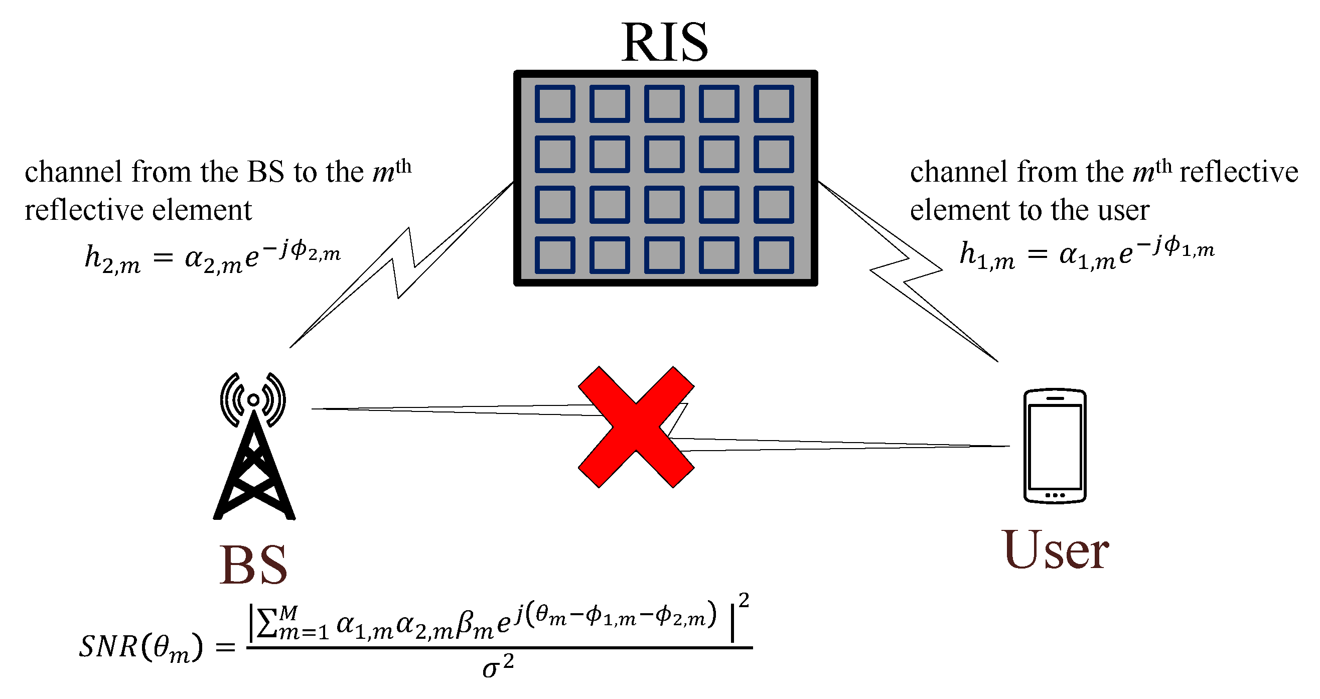
2. RIS Resource Allocation Examples and General Formulation
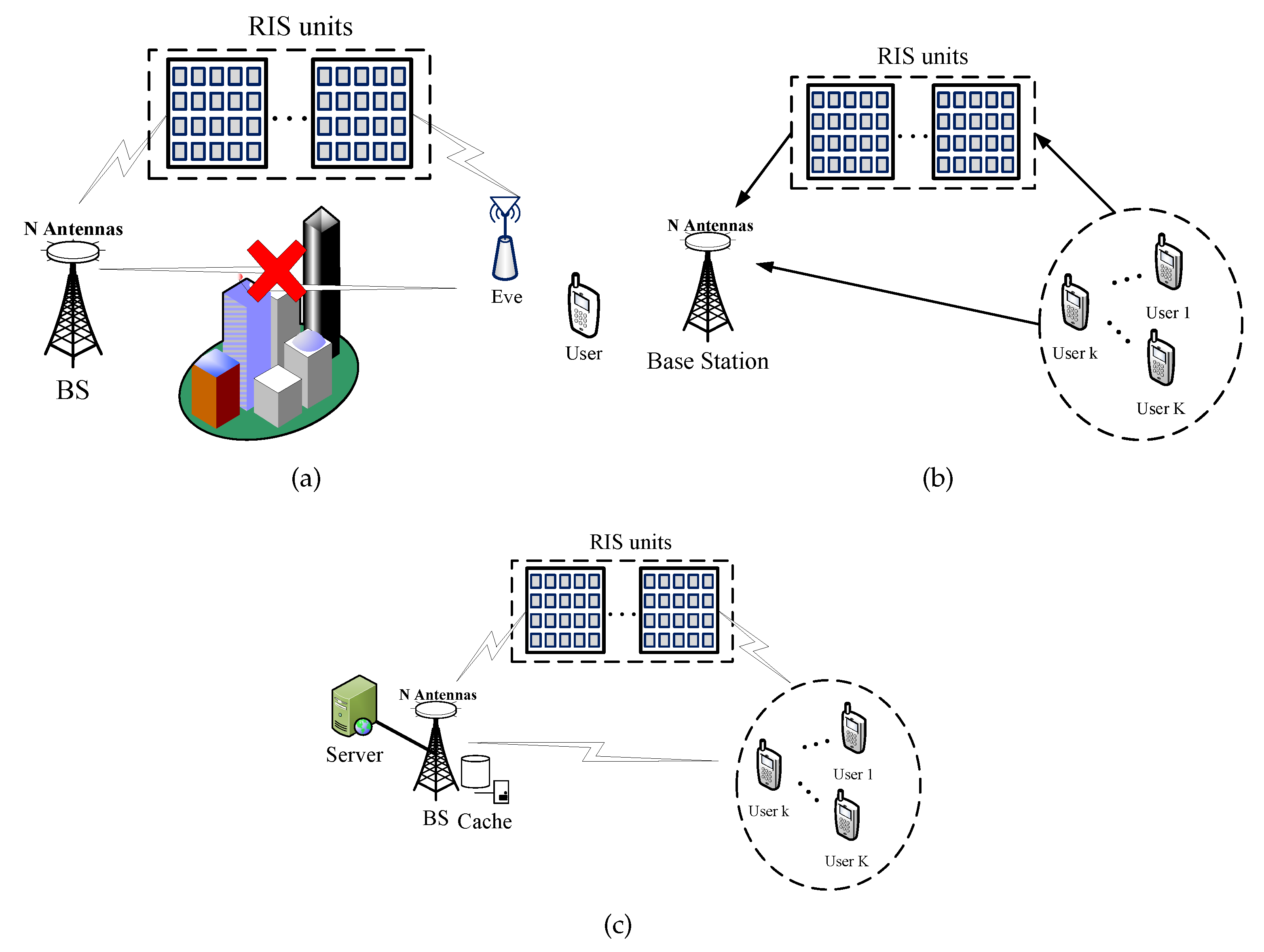
- Secure beamforming for multiple-input single-output (MISO) systems [20]: As shown in Figure 3a, the BS communicates with a single-antenna user with the help of an RIS in the presence of a single-antenna eavesdropper. The goal is to maximize the achievable secrecy rate by jointly optimizing the beamformer at the BS and the phase shift coefficients of the RIS under the transmit power constraint at the BS. To be specific, let the channels from the BS to the RIS, from the RIS to user, from the RIS to eavesdropper, and the beamforming vector at the BS be, respectively, denoted by , , , and . Then, the secrecy rate maximization problem is given bywhere is the variance of white Gaussian noise at the user.
- MISO uplink communication networks [21]: There are a number of single-antenna mobile users transmitting signals to a multi-antenna BS with the assistance of an RIS as shown in Figure 3b. The objective is to minimize the total uplink transmit power by jointly optimizing the phase shift coefficients of the RIS , the transmission power of the user k under the limited transmission power , and the signal-to-interference-and-noise-ratio (SINR) constraints. Let the channels from the BS to the RIS, from the RIS to user k, and from the BS to user k be, respectively, denoted by , , with . Accordingly, the weighted power minimization problem is given bywhere is the equivalent channel from user k to the BS, represents the weights for mobile users, and is the minimum SINR requested by the user k.
- Computation offloading in Internet of Things (IoT) networks [22]: In the downlink transmission of an RIS-aided cache-enabled radio access network, a multi-antenna BS transmits signals to a number of single-antenna users as shown in Figure 3c. The goal is to minimize the total network cost that consists of both the backhaul capacity and the transmission power by adjusting the caching proportion of the file requested by user k, the precoding vector at the BS for user k, and the RIS coefficients. In addition, the constraint on the RIS coefficients, we also have a constraint on the size of total cached content to be smaller than the local storage size at the BS. Further letting the target rate of user k be denoted by , the total network cost minimization problem is formulated aswhere is a regularization parameter, -1 is the SINR requirement in terms of the content-delivery target rate of user k, B is the bandwidth of the system, and is defined as in the previous example.
- Continuous phase shift: Each RIS coefficient has infinite phase resolution, i.e., is expressed as with i being the imaginary unit, and as a real number. For , there are three variations in the literature.
- –
- –
- –
- C3. is a function of . This is a relatively new model and takes the hardware properties into consideration. For example, one of the recent models [42] states thatwhere , and are known constants related to the specific circuit implementation.
- Discrete phase shift: Each RIS coefficient can only take one of the L possible phase shift values.
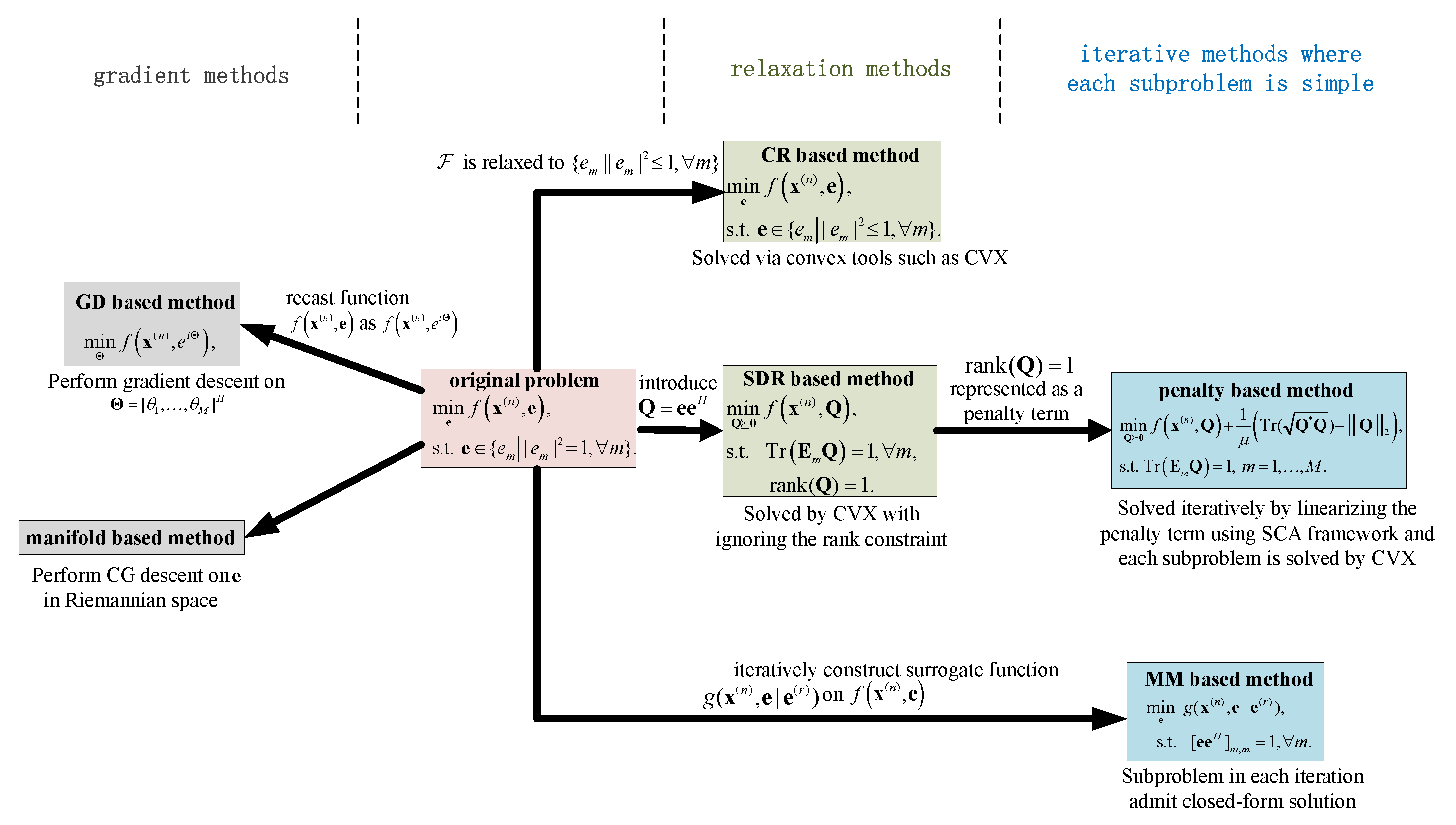
3. Review on Optimization Methods under Continuous Phase Shift
3.1. SDR Method
3.2. Penalty Method
3.3. MM Method
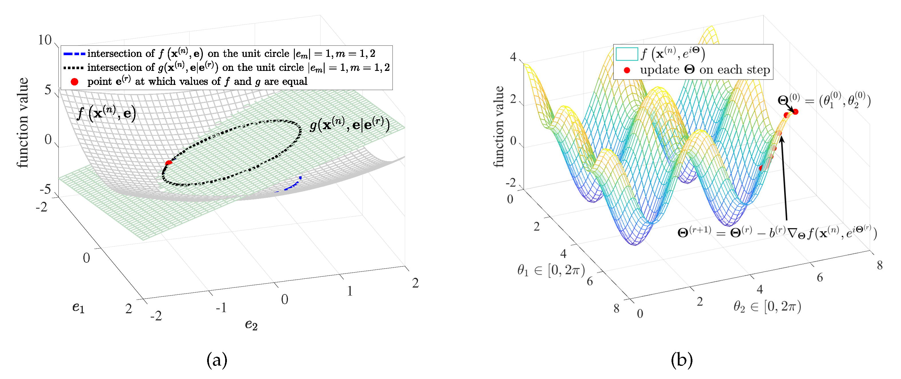
3.4. GD Method
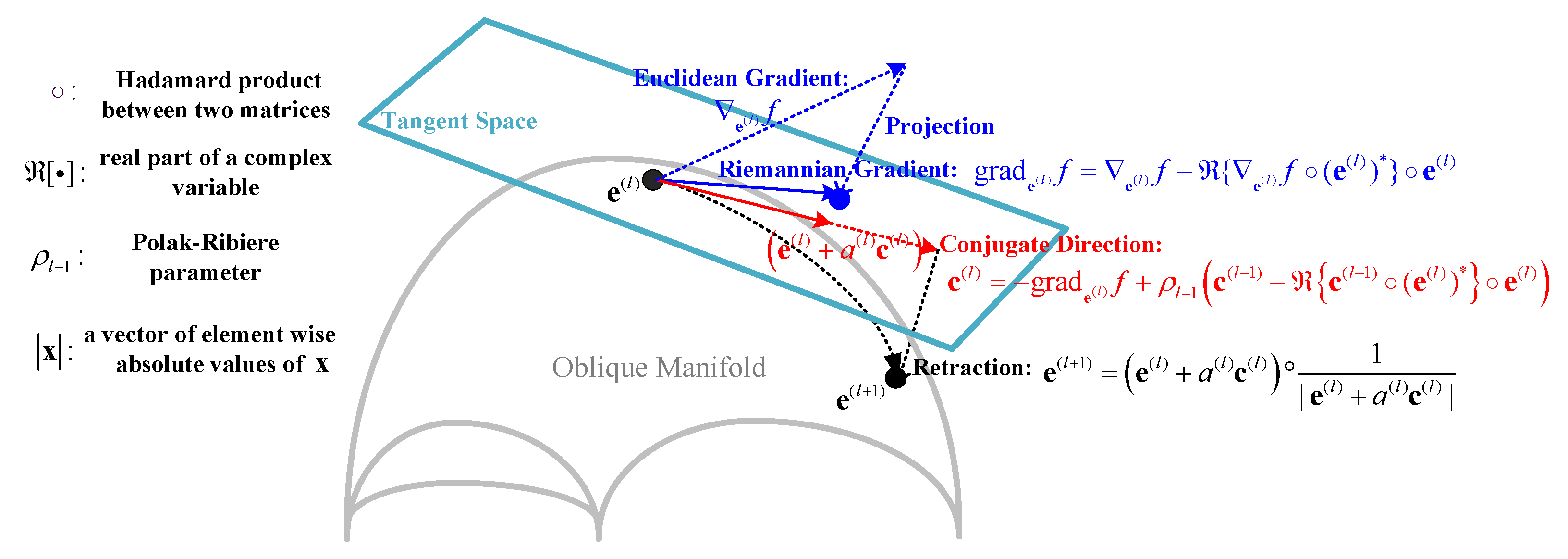
3.5. Manifold Method
3.6. CR Method
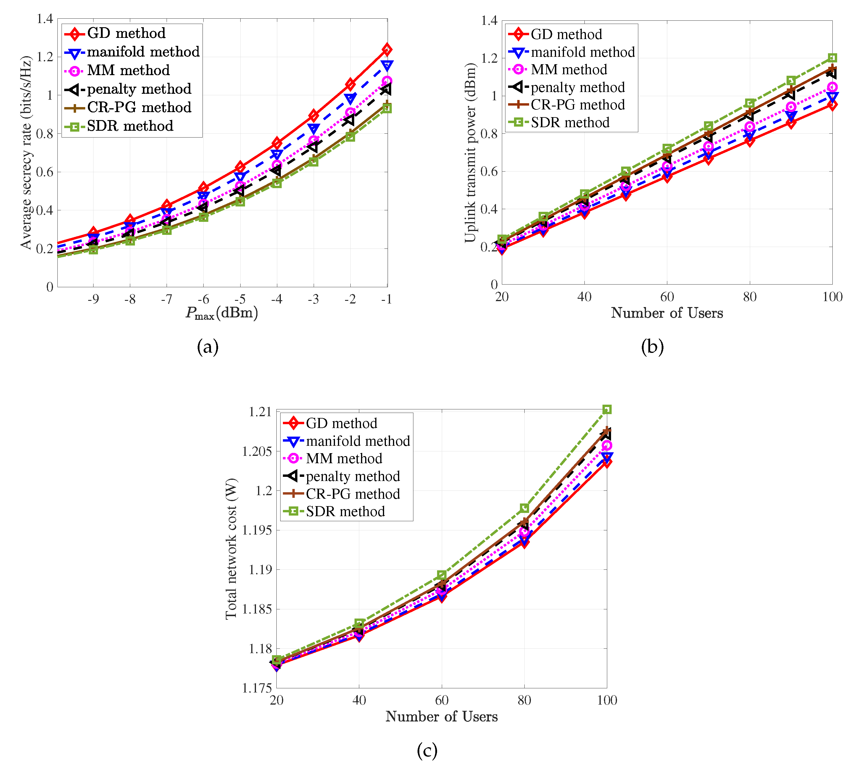
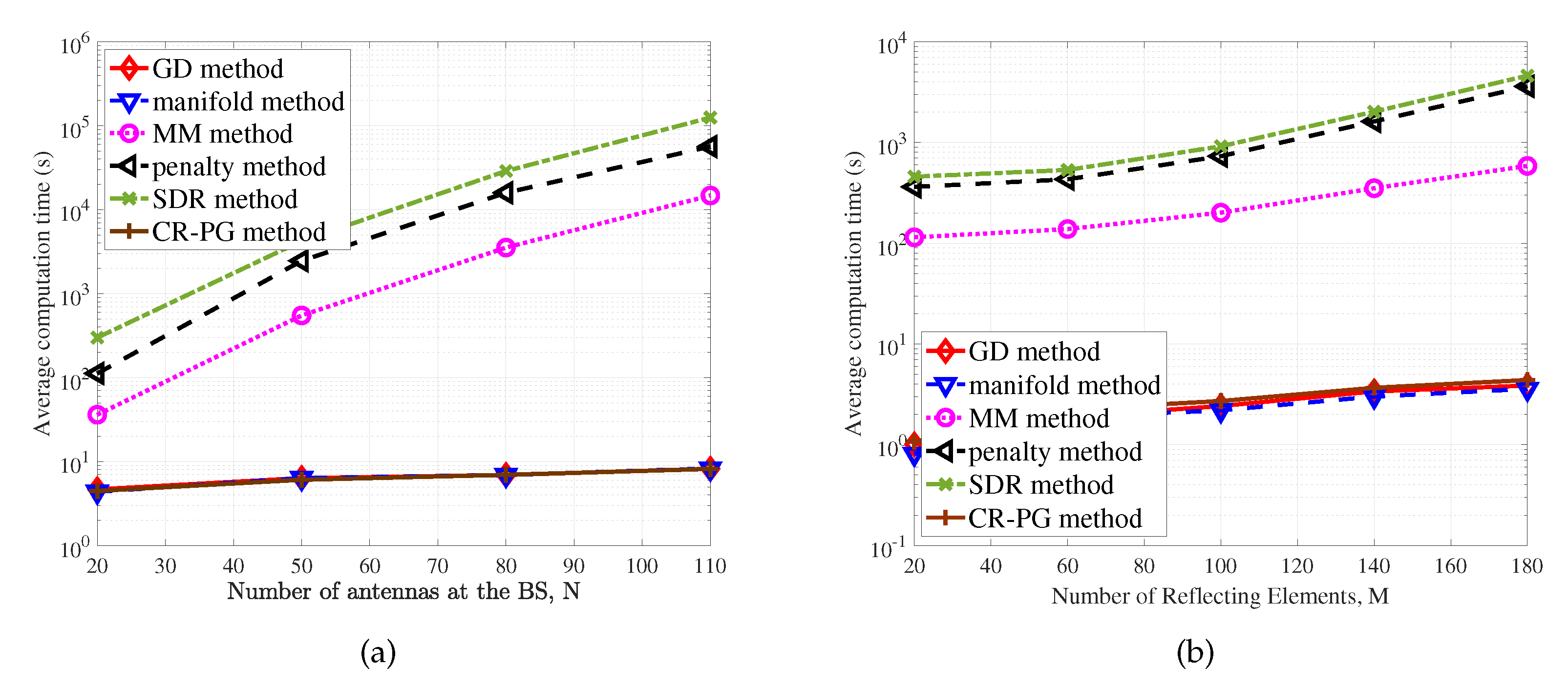
3.7. Summary and Performance Comparison
4. Learning to Optimize An RIS
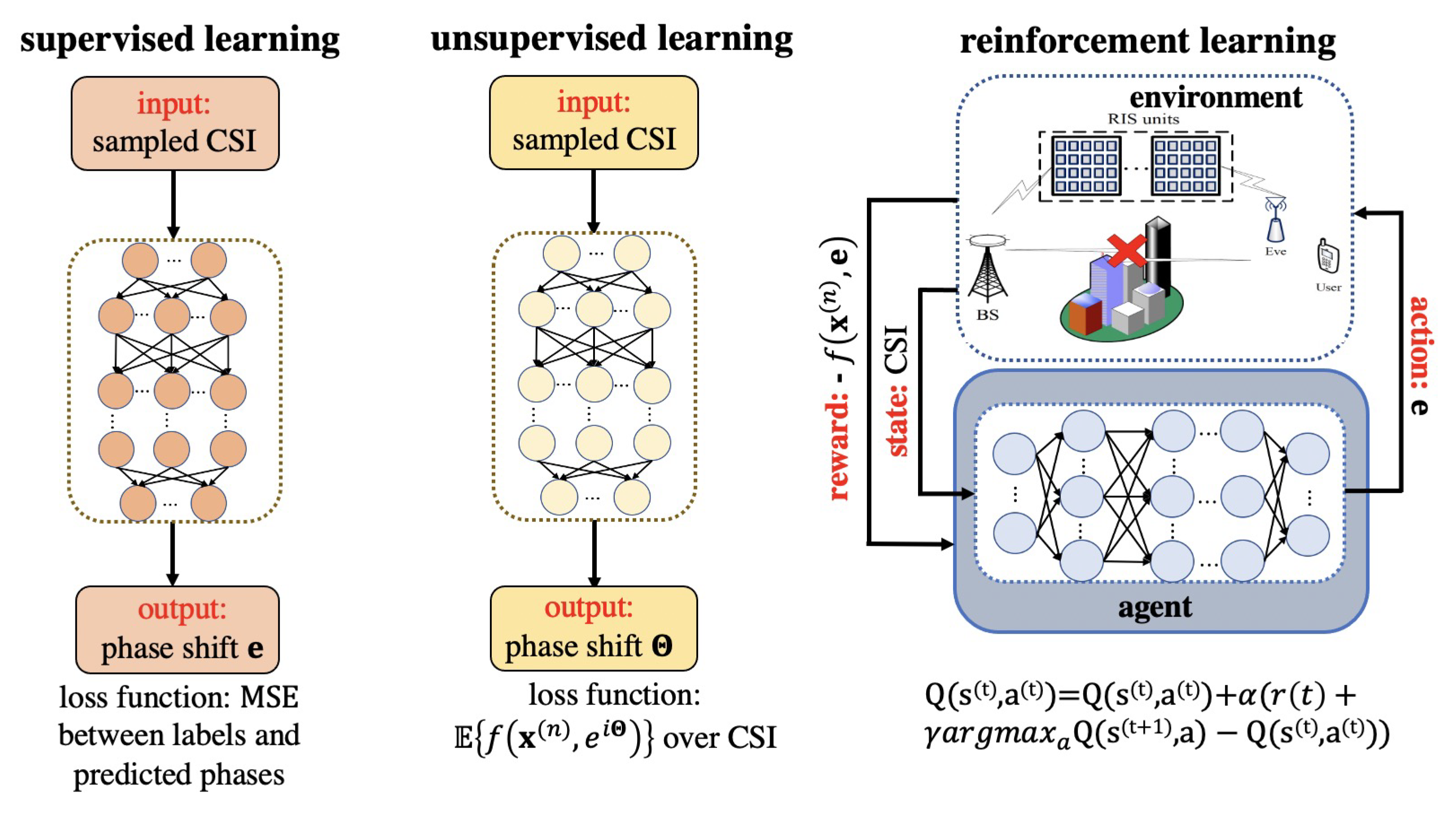
4.1. Supervised Learning
4.2. Unsupervised Learning
4.3. Reinforcement Learning
- State: a set, denoted by S, characterizing the environment. The state denotes the environment at the time step t.
- : a set of allowable actions, denoted by A. Once the agent takes an action at time instant t (determined by the state action value function), the state of the environment will transit from the current state to the next state .
- : the performance metric of a particular action, denoted by at time instant t.
- : while the reward represents the immediate return from action a at state s, the state action value function indicates cumulative rewards the agent may get from taking action a in the state s, which is denoted by .
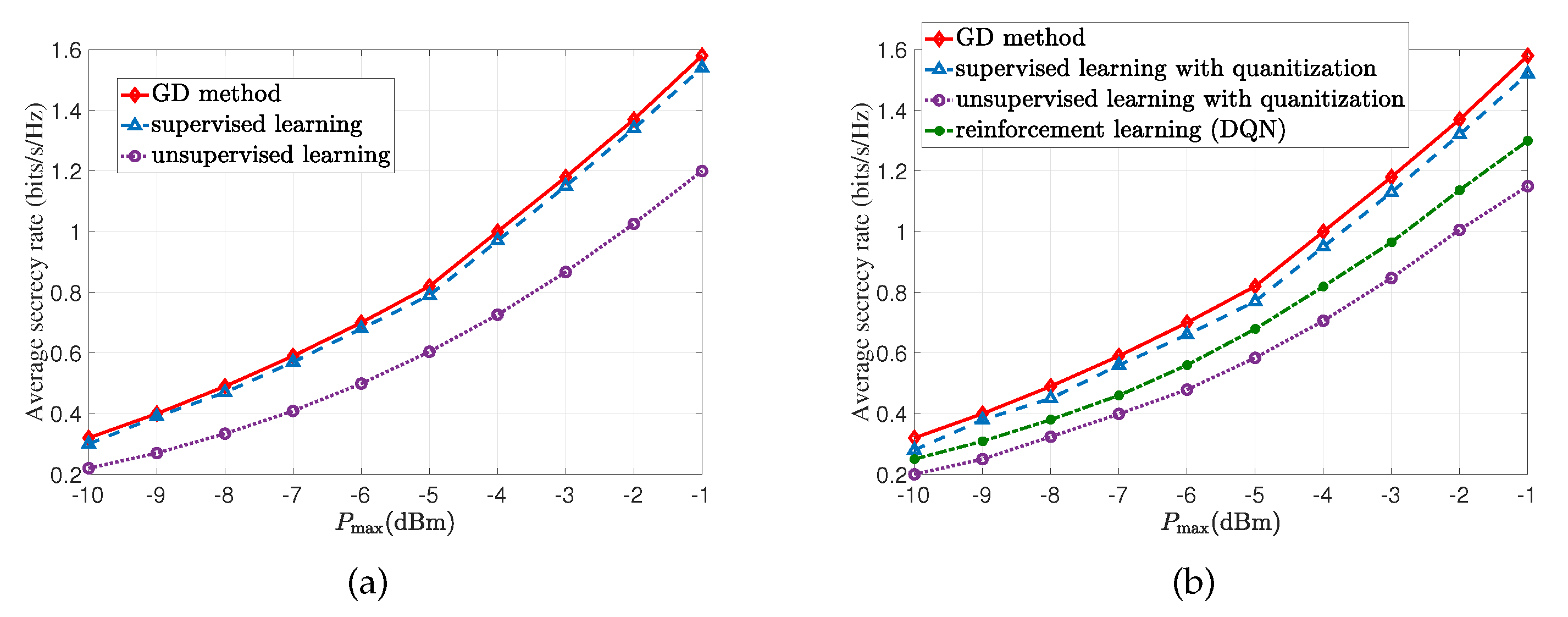
4.4. Summary and Performance Comparison
5. Future Challenges
5.1. Handling Channel Uncertainty
5.2. Handling Discrete Phase Shift
5.3. Handling the Mobility of RISs and Users
5.4. Scalability of AI-Based Methods
6. Conclusions
Author Contributions
Funding
Institutional Review Board Statement
Informed Consent Statement
Data Availability Statement
Conflicts of Interest
References
- Wu, Q.; Zhang, S.; Zheng, B.; You, C.; Zhang, R. Intelligent Reflecting Surface-Aided Wireless Communications: A Tutorial. IEEE Trans. Commun. 2021, 69, 3313–3351. [Google Scholar] [CrossRef]
- Di Renzo, M.; Ntontin, K.; Song, J.; Danufane, F.H.; Qian, X.; Lazarakis, F.; De Rosny, J.; Phan-Huy, D.T.; Simeone, O.; Zhang, R.; et al. Reconfigurable Intelligent Surfaces vs. Relaying: Differences, Similarities, and Performance Comparison. IEEE Open J. Commun. Soc. 2020, 1, 798–807. [Google Scholar] [CrossRef]
- Huang, C.; Zappone, A.; Alexandropoulos, G.C.; Debbah, M.; Yuen, C. Reconfigurable Intelligent Surfaces for Energy Efficiency in Wireless Communication. IEEE Trans. Wirel. Commun. 2019, 18, 4157–4170. [Google Scholar] [CrossRef] [Green Version]
- Dosovitskiy, A.; Ros, G.; Codevilla, F.; Lopez, A.; Koltun, V. CARLA: An open urban driving simulator. In Proceedings of the first Conference on Robot Learning (CoRL 2017), Mountain View, CA, USA, 13–15 November 2017; pp. 1–16. [Google Scholar]
- Wu, Q.; Zhang, R. Towards Smart and Reconfigurable Environment: Intelligent Reflecting Surface Aided Wireless Network. IEEE Commun. Mag. 2020, 58, 106–112. [Google Scholar] [CrossRef] [Green Version]
- Basar, E.; Di Renzo, M.; De Rosny, J.; Debbah, M.; Alouini, M.S.; Zhang, R. Wireless Communications Through Reconfigurable Intelligent Surfaces. IEEE Access 2019, 7, 116753–116773. [Google Scholar] [CrossRef]
- Jian, M.; Alexandropoulos, G.C.; Basar, E.; Huang, C.; Liu, R.; Liu, Y.; Yuen, C. Reconfigurable intelligent surfaces for wireless communications: Overview of hardware designs, channel models, and estimation techniques. Intell. Converg. Netw. 2022, 3, 1–32. [Google Scholar] [CrossRef]
- Liang, Y.C.; Long, R.; Zhang, Q.; Chen, J.; Cheng, H.V.; Guo, H. Large Intelligent Surface/Antennas (LISA): Making Reflective Radios Smart. J. Commun. Inf. Netw. 2019, 4, 40–50. [Google Scholar] [CrossRef]
- Liaskos, C.; Nie, S.; Tsioliaridou, A.; Pitsillides, A.; Ioannidis, S.; Akyildiz, I. A New Wireless Communication Paradigm through Software-Controlled Metasurfaces. IEEE Commun. Mag. 2018, 56, 162–169. [Google Scholar] [CrossRef] [Green Version]
- Huang, C.; Hu, S.; Alexandropoulos, G.C.; Zappone, A.; Yuen, C.; Zhang, R.; Renzo, M.D.; Debbah, M. Holographic MIMO Surfaces for 6G Wireless Networks: Opportunities, Challenges, and Trends. IEEE Wirel. Commun. 2020, 27, 118–125. [Google Scholar] [CrossRef]
- Di Renzo, M.; Zappone, A.; Debbah, M.; Alouini, M.S.; Yuen, C.; de Rosny, J.; Tretyakov, S. Smart Radio Environments Empowered by Reconfigurable Intelligent Surfaces: How It Works, State of Research, and The Road Ahead. IEEE J. Sel. Areas Commun. 2020, 38, 2450–2525. [Google Scholar] [CrossRef]
- Yuan, X.; Zhang, Y.J.A.; Shi, Y.; Yan, W.; Liu, H. Reconfigurable-Intelligent-Surface Empowered Wireless Communications: Challenges and Opportunities. IEEE Wirel. Commun. 2021, 28, 136–143. [Google Scholar] [CrossRef]
- Sun, Y.; Babu, P.; Palomar, D.P. Majorization-Minimization Algorithms in Signal Processing, Communications, and Machine Learning. IEEE Trans. Signal Process. 2017, 65, 794–816. [Google Scholar] [CrossRef]
- Absil, P.A.; Mahony, R.; Sepulchre, R. Optimization Algorithms on Matrix Manifolds; Princeton University Press: Princeton, NJ, USA, 2009. [Google Scholar]
- Ma, Y.; Shen, Y.; Yu, X.; Zhang, J.; Song, S.H.; Letaief, K.B. A Low-Complexity Algorithmic Framework for Large-Scale IRS-Assisted Wireless Systems. arXiv 2020, arXiv:2008.00769. [Google Scholar]
- Chen, J.; Liang, Y.C.; Pei, Y.; Guo, H. Intelligent Reflecting Surface: A Programmable Wireless Environment for Physical Layer Security. IEEE Access 2019, 7, 82599–82612. [Google Scholar] [CrossRef]
- Gao, J.; Zhong, C.; Chen, X.; Lin, H.; Zhang, Z. Unsupervised Learning for Passive Beamforming. IEEE Commun. Lett. 2020, 24, 1052–1056. [Google Scholar] [CrossRef] [Green Version]
- Taha, A.; Alrabeiah, M.; Alkhateeb, A. Deep Learning for Large Intelligent Surfaces in Millimeter Wave and Massive MIMO Systems. In Proceedings of the IEEE Global Communication Conference, Waikoloa, HI, USA, 9–13 December 2019; pp. 1–6. [Google Scholar]
- Huang, C.; Mo, R.; Yuen, C. Reconfigurable Intelligent Surface Assisted Multiuser MISO Systems Exploiting Deep Reinforcement Learning. IEEE J. Sel. Areas Commun. 2020, 38, 1839–1850. [Google Scholar] [CrossRef]
- Lu, X.; Yang, W.; Guan, X.; Wu, Q.; Cai, Y. Robust and Secure Beamforming for Intelligent Reflecting Surface Aided mmWave MISO Systems. IEEE Wirel. Commun. Lett. 2020, 9, 2068–2072. [Google Scholar] [CrossRef]
- Liu, Y.; Zhao, J.; Li, M.; Wu, Q. Intelligent Reflecting Surface Aided MISO Uplink Communication Network: Feasibility and Power Minimization for Perfect and Imperfect CSI. IEEE Trans. Commun. 2020, 69, 1975–1989. [Google Scholar] [CrossRef]
- Chen, Y.; Wen, M.; Basar, E.; Wu, Y.C.; Wang, L.; Liu, W. Exploiting Reconfigurable Intelligent Surfaces in Edge Caching: Joint Hybrid Beamforming and Content Placement Optimization. IEEE Trans. Wirel. Commun. 2021, 20, 7799–7812. [Google Scholar] [CrossRef]
- Wu, Q.; Zhang, R. Intelligent Reflecting Surface Enhanced Wireless Network via Joint Active and Passive Beamforming. IEEE Trans. Wirel. Commun. 2019, 18, 5394–5409. [Google Scholar] [CrossRef] [Green Version]
- You, C.; Zheng, B.; Zhang, R. Channel Estimation and Passive Beamforming for Intelligent Reflecting Surface: Discrete Phase Shift and Progressive Refinement. IEEE J. Sel. Areas Commun. 2020, 38, 2604–2620. [Google Scholar] [CrossRef]
- Yu, X.; Xu, D.; Sun, Y.; Ng, D.W.K.; Schober, R. Robust and Secure Wireless Communications via Intelligent Reflecting Surfaces. IEEE J. Sel. Areas Commun. 2020, 38, 2637–2652. [Google Scholar] [CrossRef]
- Zhao, M.M.; Liu, A.; Zhang, R. Outage-Constrained Robust Beamforming for Intelligent Reflecting Surface Aided Wireless Communication. IEEE Trans. Signal Process. 2021, 69, 1301–1316. [Google Scholar] [CrossRef]
- Wang, H.M.; Bai, J.; Dong, L. Intelligent Reflecting Surfaces Assisted Secure Transmission Without Eavesdropper’s CSI. IEEE Signal Process. Lett. 2020, 27, 1300–1304. [Google Scholar] [CrossRef]
- Nadeem, Q.U.A.; Kammoun, A.; Chaaban, A.; Debbah, M.; Alouini, M.S. Asymptotic Max-Min SINR Analysis of Reconfigurable Intelligent Surface Assisted MISO Systems. IEEE Trans. Wirel. Commun. 2020, 19, 7748–7764. [Google Scholar] [CrossRef] [Green Version]
- Liu, Y.; Liu, E.; Wang, R.; Geng, Y. Beamforming Designs and Performance Evaluations for Intelligent Reflecting Surface Enhanced Wireless Communication System with Hardware Impairments. arXiv 2020, arXiv:2006.00664. [Google Scholar]
- Feng, K.; Li, X.; Han, Y.; Jin, S.; Chen, Y. Physical Layer Security Enhancement Exploiting Intelligent Reflecting Surface. IEEE Commun. Lett. 2021, 25, 734–738. [Google Scholar] [CrossRef]
- Guo, H.; Liang, Y.C.; Chen, J.; Larsson, E.G. Weighted Sum-Rate Optimization for Intelligent Reflecting Surface Enhanced Wireless Networks. arXiv 2019, arXiv:1905.07920. [Google Scholar]
- Wu, Q.; Zhang, R. Joint Active and Passive Beamforming Optimization for Intelligent Reflecting Surface Assisted SWIPT Under QoS Constraints. IEEE J. Sel. Areas Commun. 2020, 38, 1735–1748. [Google Scholar] [CrossRef]
- Li, Y.; Xia, M.; Wu, Y.C. First-Order Algorithm for Content-Centric Sparse Multicast Beamforming in Large-Scale C-RAN. IEEE Trans. Wirel. Commun. 2018, 17, 5959–5974. [Google Scholar] [CrossRef]
- Li, Z.; Wang, S.; Mu, P.; Wu, Y.C. Probabilistic Constrained Secure Transmissions: Variable-Rate Design and Performance Analysis. IEEE Trans. Wirel. Commun. 2020, 19, 2543–2557. [Google Scholar] [CrossRef]
- Wang, S.; Hong, Y.; Wang, R.; Hao, Q.; Wu, Y.C.; Ng, D.W.K. Edge Federated Learning Via Unit-Modulus Over-The-Air Computation. IEEE Trans. Commun. 2022, 70, 3141–3156. [Google Scholar] [CrossRef]
- Li, Y.; Xia, M.; Wu, Y.C. Energy-Efficient Precoding for Non-Orthogonal Multicast and Unicast Transmission via First-Order Algorithm. IEEE Trans. Wirel. Commun. 2019, 18, 4590–4604. [Google Scholar] [CrossRef]
- Li, Y.; Xia, M.; Wu, Y.C. Caching at Base Stations With Multi-Cluster Multicast Wireless Backhaul via Accelerated First-Order Algorithms. IEEE Trans. Wirel. Commun. 2020, 19, 2920–2933. [Google Scholar] [CrossRef] [Green Version]
- Hu, X.; Masouros, C.; Wong, K.K. Reconfigurable Intelligent Surface Aided Mobile Edge Computing: From Optimization-Based to Location-Only Learning-Based Solutions. IEEE Trans. Commun. 2021, 69, 3709–3725. [Google Scholar] [CrossRef]
- Hua, S.; Zhou, Y.; Yang, K.; Shi, Y.; Wang, K. Reconfigurable Intelligent Surface for Green Edge Inference. IEEE Trans. Green Commun. Netw. 2021, 5, 964–979. [Google Scholar] [CrossRef]
- Yang, H.; Chen, X.; Yang, F.; Xu, S.; Cao, X.; Li, M.; Gao, J. Design of Resistor-Loaded Reflectarray Elements for Both Amplitude and Phase Control. IEEE Antennas Wirel. Propag. Lett. 2017, 16, 1159–1162. [Google Scholar] [CrossRef]
- Zhao, M.M.; Wu, Q.; Zhao, M.J.; Zhang, R. Exploiting Amplitude Control in Intelligent Reflecting Surface Aided Wireless Communication With Imperfect CSI. IEEE Trans. Commun. 2021, 69, 4216–4231. [Google Scholar] [CrossRef]
- Abeywickrama, S.; Zhang, R.; Wu, Q.; Yuen, C. Intelligent Reflecting Surface: Practical Phase Shift Model and Beamforming Optimization. IEEE Trans. Commun. 2020, 68, 5849–5863. [Google Scholar] [CrossRef]
- Wu, Q.; Zhang, R. Beamforming Optimization for Wireless Network Aided by Intelligent Reflecting Surface With Discrete Phase Shifts. IEEE Trans. Commun. 2020, 68, 1838–1851. [Google Scholar] [CrossRef] [Green Version]
- Li, N.; Li, M.; Liu, Y.; Yuan, C.; Tao, X. Intelligent Reflecting Surface Assisted NOMA With Heterogeneous Internal Secrecy Requirements. IEEE Wirel. Commun. Lett. 2021, 10, 1103–1107. [Google Scholar] [CrossRef]
- Luo, Z.; Ma, W.; So, A.M.; Ye, Y.; Zhang, S. Semidefinite Relaxation of Quadratic Optimization Problems. IEEE Signal Process. Mag. 2010, 27, 20–34. [Google Scholar] [CrossRef]
- Nocedal, J.; Wright, S. Numerical Optimization; Springer: New York, NY, USA, 2006. [Google Scholar]
- Shi, Y.; Zhang, J.; Chen, W.; Letaief, K.B. Generalized Sparse and Low-Rank Optimization for Ultra-Dense Networks. IEEE Commun. Mag. 2018, 56, 42–48. [Google Scholar] [CrossRef] [Green Version]
- Li, Z.; Xia, M.; Wen, M.; Wu, Y.C. Massive Access in Secure NOMA under Imperfect CSI: Security Guaranteed Sum-Rate Maximization with First-Order Algorithm. IEEE J. Sel. Areas Commun. 2021, 39, 998–1014. [Google Scholar] [CrossRef]
- He, X.; Wu, Y.C. Set Squeezing Procedure for Quadratically Perturbed Chance-Constrained Programming. IEEE Trans. Signal Process. 2021, 69, 682–694. [Google Scholar] [CrossRef]
- Li, Z.; Wang, S.; Wen, M.; Wu, Y.C. Secure Multicast Energy-Efficiency Maximization with Massive RISs and Uncertain CSI: First-Order Algorithms and Convergence Analysis. IEEE Trans. Wirel. Commun. 2022, 2022, 1. [Google Scholar] [CrossRef]
- Luedtke, J.; Ahmed, S. A sample approximation approach for optimization with probabilistic constraints. SIAM J. Optim. 2008, 19, 674–699. [Google Scholar] [CrossRef] [Green Version]
- Di, B.; Zhang, H.; Song, L.; Li, Y.; Han, Z.; Poor, H.V. Hybrid Beamforming for Reconfigurable Intelligent Surface based Multi-User Communications: Achievable Rates With Limited Discrete Phase Shifts. IEEE J. Sel. Areas Commun. 2020, 38, 1809–1822. [Google Scholar] [CrossRef]
- Li, Y.; Xia, M.; Wu, Y.C. Activity Detection for Massive Connectivity Under Frequency Offsets via First-Order Algorithms. IEEE Trans. Wirel. Commun. 2019, 18, 1988–2002. [Google Scholar] [CrossRef]
- Tibshirani, R. Regression shrinkage and selection via the Lasso: A retrospective Series B Statistical methodology. J. R. Stat. Soc. 2011, 73, 273–282. [Google Scholar] [CrossRef]
- Shao, M.; Li, Q.; Ma, W.K.; Thus, A.M.C. A Framework for One-Bit and Constant-Envelope Precoding Over Multiuser Massive MISO Channels. IEEE Trans. Signal Process. 2019, 67, 5309–5324. [Google Scholar] [CrossRef] [Green Version]
- Pan, C.; Ren, H.; Wang, K.; Kolb, J.F.; Elkashlan, M.; Chen, M.; Di Renzo, M.; Hao, Y.; Wang, J.; Swindlehurst, A.L.; et al. Reconfigurable Intelligent Surfaces for 6G Systems: Principles, Applications, and Research Directions. IEEE Commun. Mag. 2021, 59, 14–20. [Google Scholar] [CrossRef]
- Powell, W.B. Approximate Dynamic Programming: Solving the Curses of Dimensionality; John Wiley & Sons: Hoboken, NJ, USA, 2007. [Google Scholar]
- Yang, H.; Xiong, Z.; Zhao, J.; Niyato, D.; Xiao, L.; Wu, Q. Deep Reinforcement Learning-Based Intelligent Reflecting Surface for Secure Wireless Communications. IEEE Trans. Wirel. Commun. 2021, 20, 375–388. [Google Scholar] [CrossRef]
- Ma, Y.; Shen, Y.; Yu, X.; Zhang, J.; Song, S.; Letaief, K.B. Neural Calibration for Scalable Beamforming in FDD Massive MIMO with Implicit Channel Estimation. In Proceedings of the IEEE Global Communication Conference, Waikoloa, HI, USA, 9–13 December 2019; pp. 1–6. [Google Scholar]
- Shen, Y.; Shi, Y.; Zhang, J.; Letaief, K.B. Graph Neural Networks for Scalable Radio Resource Management: Architecture Design and Theoretical Analysis. IEEE J. Sel. Areas Commun. 2021, 39, 101–115. [Google Scholar] [CrossRef]
- Guo, J.; Yang, C. Learning Power Allocation for Multi-Cell-Multi-User Systems With Heterogeneous Graph Neural Networks. IEEE Trans. Wirel. Commun. 2022, 21, 884–897. [Google Scholar] [CrossRef]
- Li, Y.; Chen, Z.; Wang, Y.; Yang, C.; Wu, Y.C. Heterogeneous Transformer: A Scale Adaptable Neural Network Architecture for Device Activity Detection. arXiv 2021, arXiv:2112.10086. [Google Scholar]
- Li, Y.; Chen, Z.; Liu, G.; Wu, Y.C.; Wong, K.K. Learning to Construct Nested Polar Codes: An Attention-Based Set-to-Element Model. IEEE Commun. Lett. 2021, 25, 3898–3902. [Google Scholar] [CrossRef]


| Reference | Review Focuses |
|---|---|
| [2] | Differences and similarities between RIS and relay. |
| [1] | RIS-aided wireless communications and its future research. |
| [5] | RIS technology for wireless communication, and its applications. |
| [6] | State-of-the-art solutions for RIS-empowered wireless networks with an emphasis on applying RIS as multipath controller and energy-efficient transmitter. |
| [7] | Hardware designs, channel models, and channel estimation techniques for RIS-aided wireless networks. |
| [8] | The implementations, applications, and open research problems of large intelligent surface. |
| [9] | The functional and physical architecture of software-controlled metasurface and discuss its network-layer integration. |
| [10] | The holographic MIMO surface, its hardware architectures as well as main characteristics. |
| [11] | RIS applications, state-of-the-art research and future research directions. |
| [12] | RIS channel estimation, passive information transfer, and resource allocation. |
| Notation | Description |
|---|---|
| M | number of reflecting elements in RIS |
| K | number of users |
| variance of white Gaussian noise | |
| channels from BS to the RIS | |
| channels from RIS to user k | |
| channels from BS to user k | |
| equivalent channels from BS to user k | |
| vector of RIS coefficients | |
| amplitude for RIS’s reflecting element | |
| phase shift for RIS’s reflecting element | |
| rank-one auxiliary variable of |
| Optimization Methods | Property of Solutions | Complexity Order | Applicable Model | Examples |
|---|---|---|---|---|
| SDR | infeasible/feasible solution | C1 and C2 | [23,24] | |
| Penalty | stationary solution | C1 and C2 | [25,26] | |
| MM | locally optimal solution [13] | C1 and C2 | [3,27] | |
| GD | stationary solution [15] | C1, C2, and C3 | [28,29] | |
| Manifold | stationary solution [14] | C1 and C2 | [22,30] | |
| CR | feasible solution [15] | using CVX using PG | C1 and C2 | [16,31] |
| Methods | Training Data Preparation Time | Training Time | Inference Time |
|---|---|---|---|
| GD | not applicable | not applicable | 21.7 ms |
| Supervised Learning | 4.8 h | 10.521 h | 87.1 s |
| Unsupervised Learning | not applicable | 11.347 h | 66.3 s |
| Reinforcement Learning | not applicable | 17.862 h | 14.3 ms |
Publisher’s Note: MDPI stays neutral with regard to jurisdictional claims in published maps and institutional affiliations. |
© 2022 by the authors. Licensee MDPI, Basel, Switzerland. This article is an open access article distributed under the terms and conditions of the Creative Commons Attribution (CC BY) license (https://creativecommons.org/licenses/by/4.0/).
Share and Cite
Li, Z.; Wang, S.; Lin, Q.; Li, Y.; Wen, M.; Wu, Y.-C.; Poor, H.V. Phase Shift Design in RIS Empowered Wireless Networks: From Optimization to AI-Based Methods. Network 2022, 2, 398-418. https://doi.org/10.3390/network2030025
Li Z, Wang S, Lin Q, Li Y, Wen M, Wu Y-C, Poor HV. Phase Shift Design in RIS Empowered Wireless Networks: From Optimization to AI-Based Methods. Network. 2022; 2(3):398-418. https://doi.org/10.3390/network2030025
Chicago/Turabian StyleLi, Zongze, Shuai Wang, Qingfeng Lin, Yang Li, Miaowen Wen, Yik-Chung Wu, and H. Vincent Poor. 2022. "Phase Shift Design in RIS Empowered Wireless Networks: From Optimization to AI-Based Methods" Network 2, no. 3: 398-418. https://doi.org/10.3390/network2030025