Article

Estimation of Iron Loss in Permanent Magnet Synchronous Motors Based on Particle Swarm Optimization and a Recurrent Neural Network

1
School of Electrical and Data Engineering, University of Technology Sydney, Ultimo, NSW 2007, Australia
2
School of Electrical and Information Engineering, The University of Sydney, Camperdown, NSW 2006, Australia
*
Author to whom correspondence should be addressed.
Magnetism 2023, 3(4), 327-342; https://doi.org/10.3390/magnetism3040025
Submission received: 27 September 2023 / Revised: 6 December 2023 / Accepted: 7 December 2023 / Published: 11 December 2023
(This article belongs to the Special Issue Digital Twins for Magnetic Devices)

Abstract

:
The popularity of permanent magnet synchronous motors (PMSMs) has increased in recent years due to their high efficiency, compact size, and low maintenance needs. Calculating iron loss in PMSMs is crucial for designing and optimizing PMSMs to achieve high efficiency and a long lifespan, as this can significantly affect motor performance. However, multiple factors influence the accuracy of iron loss calculations in PMSMs, including the intricate magnetic behavior of the motor under different operating conditions, as well as the influence of the motor’s dynamic behavior during the operation process. This paper proposes a method based on particle swarm optimization (PSO) and a recurrent neural network (RNN) to estimate the iron loss in PMSMs, independent of the empirical iron loss formula. This method establishes an iron loss calculation model considering high-order harmonics, rotating magnetization, and temperature factors. Accounting for the multifactor influence, the model studies the law of loss change under different magnetic flux densities, frequencies, and temperature conditions. To avoid the deviation problem caused by conventional polynomial fitting, a multilayer RNN and PSO are used to train and optimize the neural network. Iron loss in complex cases beyond the measurement range can be accurately estimated. The proposed method helps achieve a PMSM iron loss calculation model with broad applicability and high accuracy.

1. Introduction

Accurately calculating iron loss in permanent magnet synchronous motors (PMSMs) is critical. Inaccurate calculations can lead to suboptimal motor designs and operations, resulting in reduced efficiency, increased energy consumption, and higher operating costs. Moreover, they contribute to overheating issues, insulation failure, premature aging, and unexpected failures, compromising motor performance and posing safety risks including potential accidents or damage to equipment and property [1,2]. Therefore, the accurate estimation of iron loss in PMSMs is crucial for ensuring optimal motor performance, energy efficiency, reliability, and longevity. It directly impacts the operational efficiency, safety, maintenance costs, and environmental footprint of systems utilizing these motors [3,4]. Understanding and minimizing iron losses are key to improving the overall efficiency of PMSMs. Accurate calculation of iron loss informs the design of more efficient PMSMs and related applications including design optimization, performance prediction and improvement, simulation and control strategy, and energy efficiency improvement.
Several existing methods are employed to estimate iron loss in PMSMs. These methods include analytical methods, finite element analysis (FEA), experimental testing, and combined approaches. Traditional analytical methods involve mathematical models and equations based on magnetic theories to estimate iron losses. These methods often rely on empirical formulas and simplified assumptions regarding the motor’s magnetic behavior under different operating conditions [5,6,7]. FEA is a numerical simulation technique that models the motor’s geometry and material properties to simulate magnetic fields and compute iron losses. It provides more detailed and accurate estimations by considering the motor’s complex geometry and nonlinear material properties [8,9,10]. Direct measurement through experimental tests involves running the motor under controlled conditions while measuring parameters such as temperature rise, electrical parameters, and loss components. However, this method is time consuming, costly and may not cover all operating scenarios [1].
Accurately calculating iron loss is a challenging issue in the industrial application of electrical machines due to the impact of saturation on the magnetic circuit and the dynamic operational modes. The main research focus in terms of PMSMs is developing precise iron loss models. The iron loss for interior PMSMs has been studied using a variety of models. There are a number of models that have been proposed that take into consideration the effect of magnetic properties on temperature, for example, the rotating magnetization model [11]. In addition, models that consider the influence on magnetic properties have been proposed, for example, the temperature model [12,13] and the mechanical stress model [14]. According to the authors in [15,16], calculations have been provided for iron loss in permanent magnet (PM) motors, considering PWM inverter harmonics as a factor in the calculation. Furthermore, efforts have been made to optimize motor design and control strategies to minimize this loss. Accurate calculation of iron loss in PMSMs refers to the ability to estimate the amount of energy dissipated in the cores due to magnetic hysteresis and eddy currents with a high degree of precision [17,18].
Currently, the accurate calculation of iron loss in PMSMs presents a formidable challenge due to several intricate factors. The complex magnetic characteristics of the iron cores, including magnetic saturation and hysteresis, pose difficulties in modeling these losses accurately. Furthermore, the dynamic behavior of PMSMs, which varies under both steady-state and transient conditions, adds to the complexity. The amount of iron loss is heavily reliant on the characteristics of the core material, including its magnetic permeability and core loss coefficients, which can fluctuate with temperature and manufacturing variations, introducing uncertainty into the calculations. The strong connection between iron loss and motor temperature requires consideration of the thermal distribution within the motor, further complicating the modeling process. Additionally, achieving precise iron loss calculations often requires specific knowledge about the motor’s design, core material properties, and manufacturing processes. However, these may not always be readily accessible, especially for custom or proprietary motors. Measuring iron loss directly in PMSMs is challenging due to the small size and intricate geometry of the motors, making experimental techniques demanding in terms of instrumentation and susceptible to measurement errors. The absence of standardized testing procedures, coupled with the constant change in motor behavior during operation, underscores the complexities involved in the accurate assessment of iron loss [19,20]. Acquiring knowledge about the correlation between the key factors that influence iron loss, and the actual magnitude of iron loss is a crucial step in accurately calculating iron loss during the creation of high-efficiency motors. These data enable the identification and proposal of targeted loss-reduction techniques.
During PMSM operation, the flux density waveform deviates from a pure sinusoidal shape due to factors such as current harmonics, nonlinear core properties, and spatial harmonics. These deviations can affect motor efficiency, torque stability, and electromagnetic compatibility [21,22,23]. This results in more severe distortion in the magnetic density wave- form, making it difficult to accurately calculate iron loss using formula-based methods. To address these challenges, motor designers and control engineers employ various strategies, including advanced controls and material selection, to optimize motor performance in real-world scenarios. A time-stepped FEA model of a motor was used to calculate the iron loss from the stator [8,9]. The coefficient to calculate iron loss is typically obtained by fitting it to the measured loss at a particular frequency and magnetic flux density [14,24]. However, a constant-coefficient model can cause a deviation in the calculation. Therefore, it is essential to investigate an iron loss model with variable coefficients that take into account alterations in the loss coefficient with magnetic flux density and frequency in order to tackle this issue [25,26].
Using an FEA model with time stepping to calculate stator iron losses in motors is a reliable and popular technique that offers a comprehensive understanding of the dynamic electromagnetic behavior within the motor [9,10]. This method involves a meticulous process, from the intricate setup of a 3D FEA model, mesh generation, and time-stepping analysis to the calculation of magnetic fields, eddy currents, and hysteresis losses. By integrating these losses over time and optionally considering thermal effects, researchers can gain valuable insights into the motor’s iron loss characteristics under varying operating conditions. While this approach is effective and powerful, it demands expertise in FEA software, such as Ansys Electronics Desktop 2023 R1 and Altair Flux 2022.2, high-performance computer hardware requirements, electromagnetics, and a profound understanding of the motor’s design and material properties. The accuracy of the results depends on precise modeling and data calibration, which may require validation against experimental measurements.
The two- and three-term variable-coefficient models have been suggested in certain studies for different silicon steel sheets. The loss coefficients in both models are subject to variation due to changes in frequency and magnetic flux density. The use of variable-coefficient models has demonstrated superior accuracy in various scenarios compared to constant-coefficient models. Variable-coefficient models excel at capturing nonuniformity, accommodating dynamic systems, addressing complex geometries, and representing physical processes more realistically. However, their increased complexity and computational demands should be considered alongside the specific needs of the analysis. The choice between constant- and variable-coefficient models should be guided by a deep understanding of the system, available data, and the desired level of precision, as both have valuable roles in scientific and engineering simulations [27,28,29,30,31]. Despite the fact that variable-coefficient models express the loss coefficient as a polynomial function of magnetic flux density and frequency, the numerical fitting process can be ill-conditioned, leading to inaccuracies when the ranges of frequency and magnetic flux density are extensive.
As part of the process of resolving the challenges related to the variable-coefficient model, previous studies have shown that when the frequency or magnetic flux density is high, the eddy current loss increases significantly as well [32,33,34]. Previous research has proposed adding an additional term to the Bertotti three-term constant-coefficient model, namely the high-order magnetic flux density term, in order to counterbalance this increase in eddy current loss. They have also proposed an iron loss model with an additional term for the eddy current [35,36]. According to the existing literature, the impact of local hysteresis loops caused by harmonic magnetic fields on iron loss has been extensively researched. It has been observed that with increases in the frequency and amplitude of the harmonic magnetic field, the influence of local hysteresis loops on iron loss also increases significantly [37,38]. Despite the widespread use of empirical formulas for calculating iron loss coefficients using polynomial fitting, accurately accounting for multiple factors such as high-order harmonic magnetic density, frequency, and temperature remains challenging. In particular, the accuracy of the results is significantly affected when the frequency or temperature is high, leading to a significant deviation.
Throughout the years, a variety of models have been employed to calculate the iron loss in PMSMs, including the Steinmetz equation and its improved version, the separation of hysteresis and eddy current loss, mathematical hysteresis models, and the division of the magnetizing process loss [39]. The Steinmetz equation is a simple empirical formula that is easy to use and suitable for basic calculations during the initial design stage. However, it has limitations in accurately representing complex magnetic materials and geometries. The Steinmetz model with eddy current loss is an extension of the original Steinmetz equation. This model offers improved accuracy by accounting for both hysteresis and eddy current losses. The Bertotti model is a more advanced mathematical approach that considers hysteresis and eddy currents in greater detail. It provides greater accuracy and is well-suited for a wide range of industrial and scientific applications [5]. Ansys Maxwell in Electronics Desktop 2023 R1 is a powerful FEA software designed for electromagnetic field simulations. It offers high fidelity, 3D modeling capabilities, extensive material libraries, and advanced analysis options. It is the tool of choice for professionals and industries where the utmost precision and comprehensive analysis are required [6]. Iron loss is typically divided into three distinct categories: hysteresis loss, eddy loss, and excess loss. Advanced iron loss calculations [7] involve fitting a known interpolation function to the measured iron loss data, allowing for the analysis of iron loss at any given flux density and frequency. Table 1 displays the expression and number of parameters of the classic iron loss models.
The Steinmetz equation involves three loss coefficients, k h , n , and m . The Bertotti loss equation, on the other hand, has three loss coefficients, k h , k c , and k e , with α being the coefficient of hysteresis loss. The magnetic field frequency is denoted by f and the magnitude of the flux density is represented by B . To improve the accuracy of the prediction in higher flux density ranges as well as for rotational fields, a model with five parameters was used. This enhanced model includes k 1 and k 2 , which are calculated based on the rotational pattern of magnetic induction. The term multiplied by α 1 represents the hysteretic losses, and the term multiplied by α 5 represents the excess losses, depending on the method used for parameterization. The two intermediate terms signify the eddy current component of the losses. It is evident that the number of parameters in the iron loss calculation formula increases with an increase in the accuracy of the iron loss calculation.
In recent times, neural network algorithms have gained significant prominence in the realm of iron loss estimation and computation. A novel neural network dynamic hysteresis model has been introduced to calculate iron losses effectively within amorphous magnetic cores in high-frequency transformers, even when subjected to non-sinusoidal magnetization conditions [40]. There has been some research undertaken to analyze the specific iron losses in cold-rolled, non-oriented electrical steel sheets, using the combination of artificial neural networks (ANNs) and genetic algorithms (GAs), covering a wide range of frequencies and magnetic flux densities [41]. In a separate application, an ANN has been employed to gauge the machine parameters essential for achieving optimal efficiency in synchronous reluctance motors. In this comprehensive model, magnetic saturation is considered, cross-coupling effects are considered, and iron losses are also included [42].
In this study, a particle swarm optimization (PSO) recurrent neural network (RNN) method is presented to analyze and estimate the iron loss of PMSM without relying on empirical iron loss formulas. The key contributions of this method can be summarized as follows:
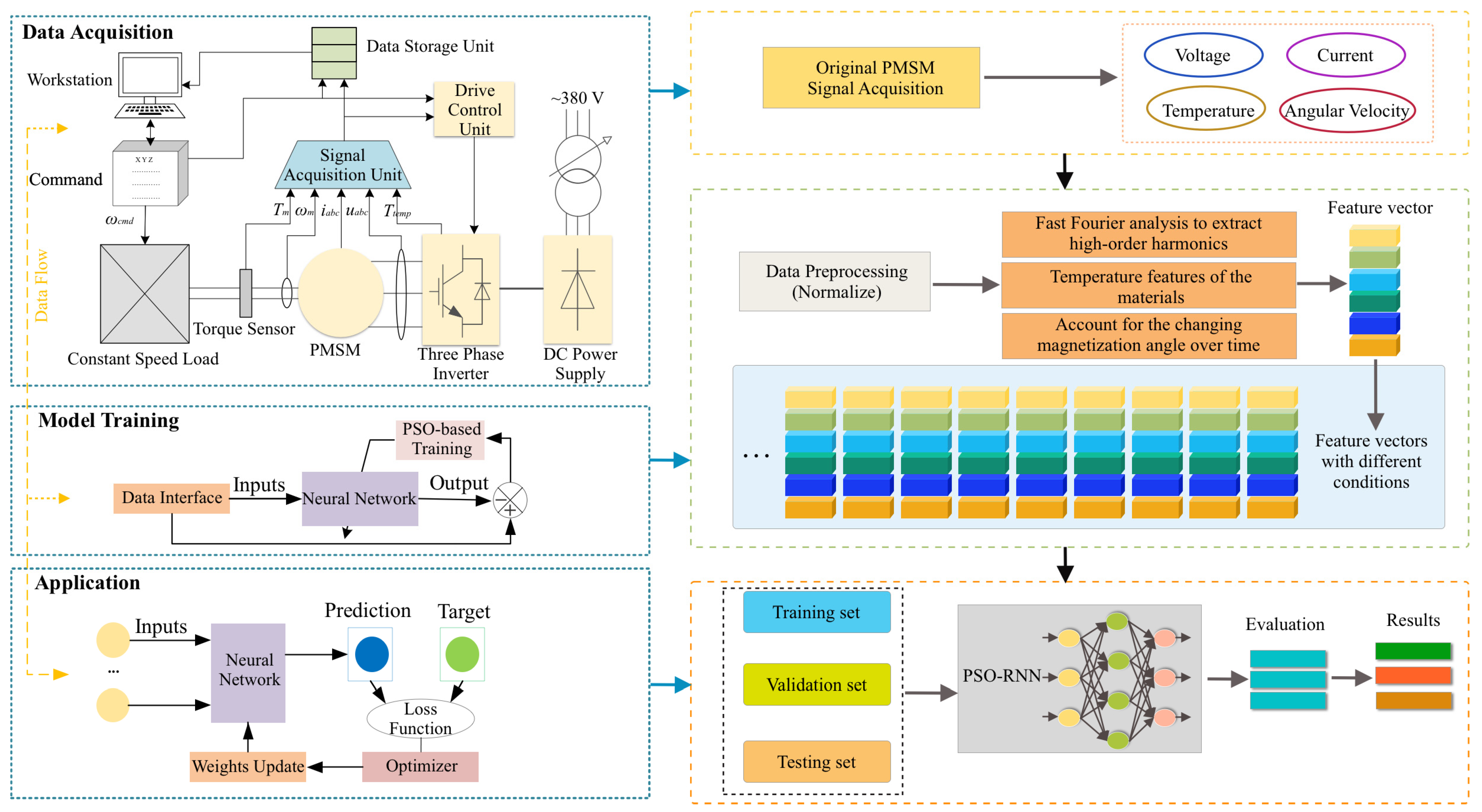
  • The proposed method integrates PSO and RNN to establish a comprehensive iron loss calculation model. This model accounts for high-order harmonics, rotating magnetization, and temperature factors, capturing multifaceted influences on iron loss.
  • By employing multilayer RNN and PSO for training and optimization, the method overcomes issues associated with conventional polynomial fitting, offering improved accuracy in estimating iron loss even in complex scenarios beyond traditional measurement ranges.
  • The developed model offers broad applicability by accurately estimating iron loss in PMSMs under diverse and complex conditions, surpassing the limitations of traditional empirical formulas.
By departing from traditional reliance on empirical iron loss formulas, this research explores the intricate impact of multiple factors on iron loss patterns. Using intelligence optimization algorithms and neural network techniques, an innovative iron loss model based on a PSO–RNN was devised, that is capable of estimating iron loss even in complex scenarios that fall beyond standard measurement ranges. The study showcases the outcomes of iron loss calculations using the PSO–RNN method. It demonstrates the successful development of a highly adaptable and precise PMSM iron loss estimation model, significantly expanding its applicability range.

2. Impact Factor Analysis of Iron Loss

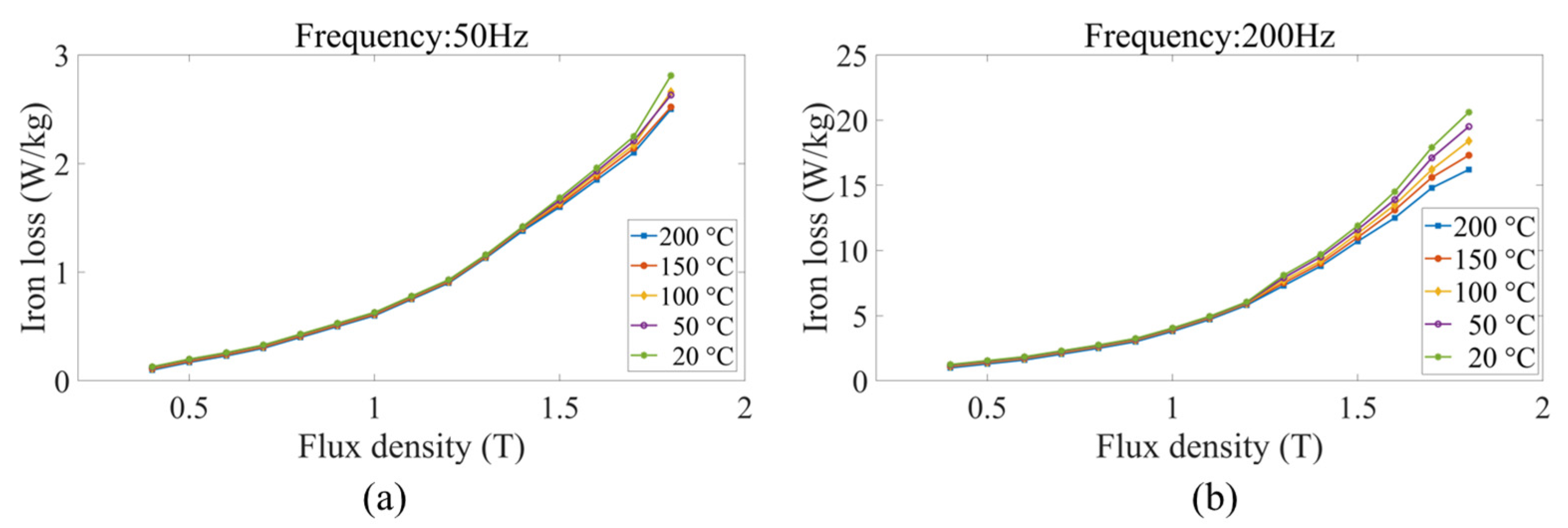
2.1. Frequencies and Temperatures

Silicon steel sheets are commonly employed as the material for the motor core. However, their magnetic properties, loss, and magnetization curves are subject to temperature effects that alter their material characteristics. As a result, these temperature effects can influence the iron loss calculation and cause deviations in the loss estimation of magnetic materials. Figure 1 presents the loss curves of a 35WW360 silicon steel sheet from 20 to 200 °C for frequencies of 50 Hz and 200 Hz [14,43,44,45]. At 50 Hz, the unit mass loss is minimally influenced by temperatures below a magnetic flux density of 1.5T, but is negatively correlated with a temperature above this value. The inflection point occurs at 1.3T, as shown in Figure 1a,b. The trends in the loss curves are the same for both frequencies. Additionally, frequency affects the proportion of loss reduction at different temperatures, with higher frequencies resulting in more significant loss reduction. The maximum ratio of loss reduction is 18.37% at 50 Hz and 20.56% at 200 Hz. This indicates that frequency plays a role in determining how temperature affects the loss per unit mass.

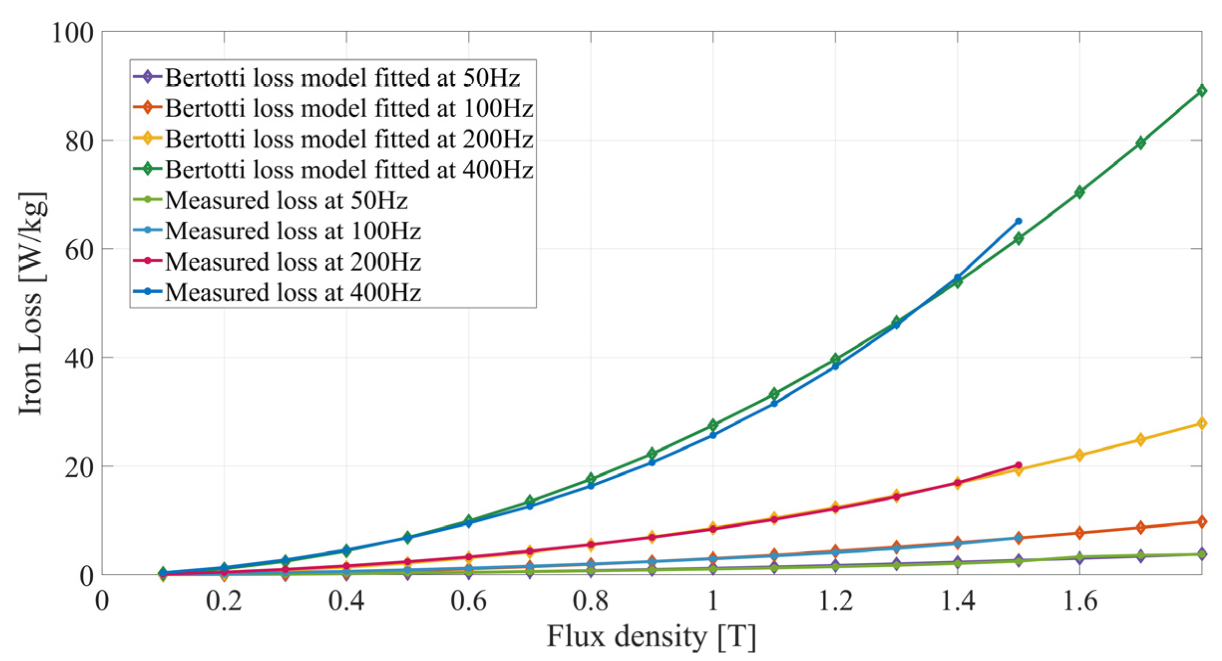
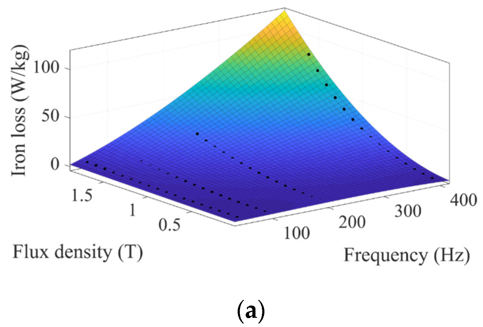
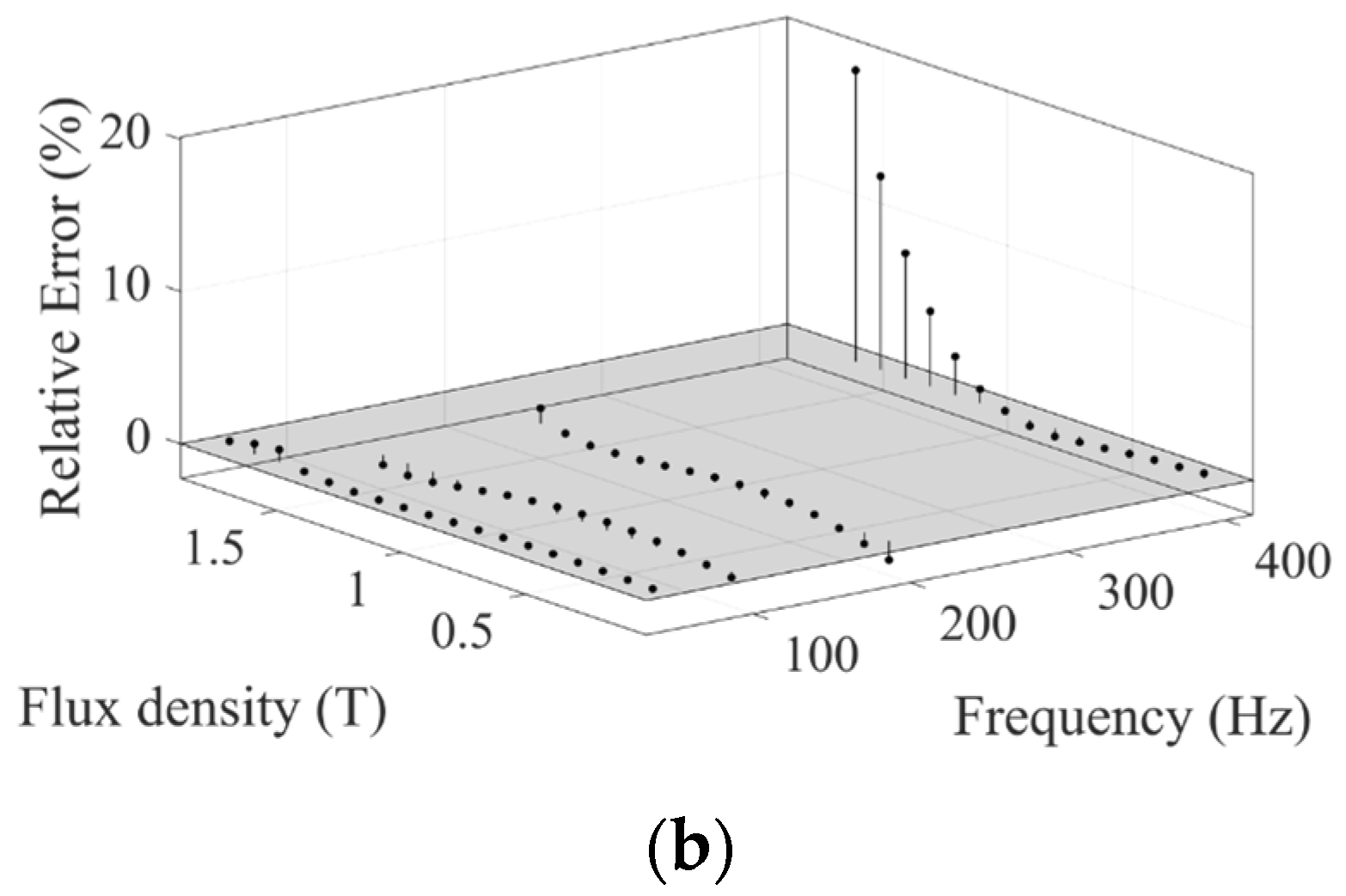
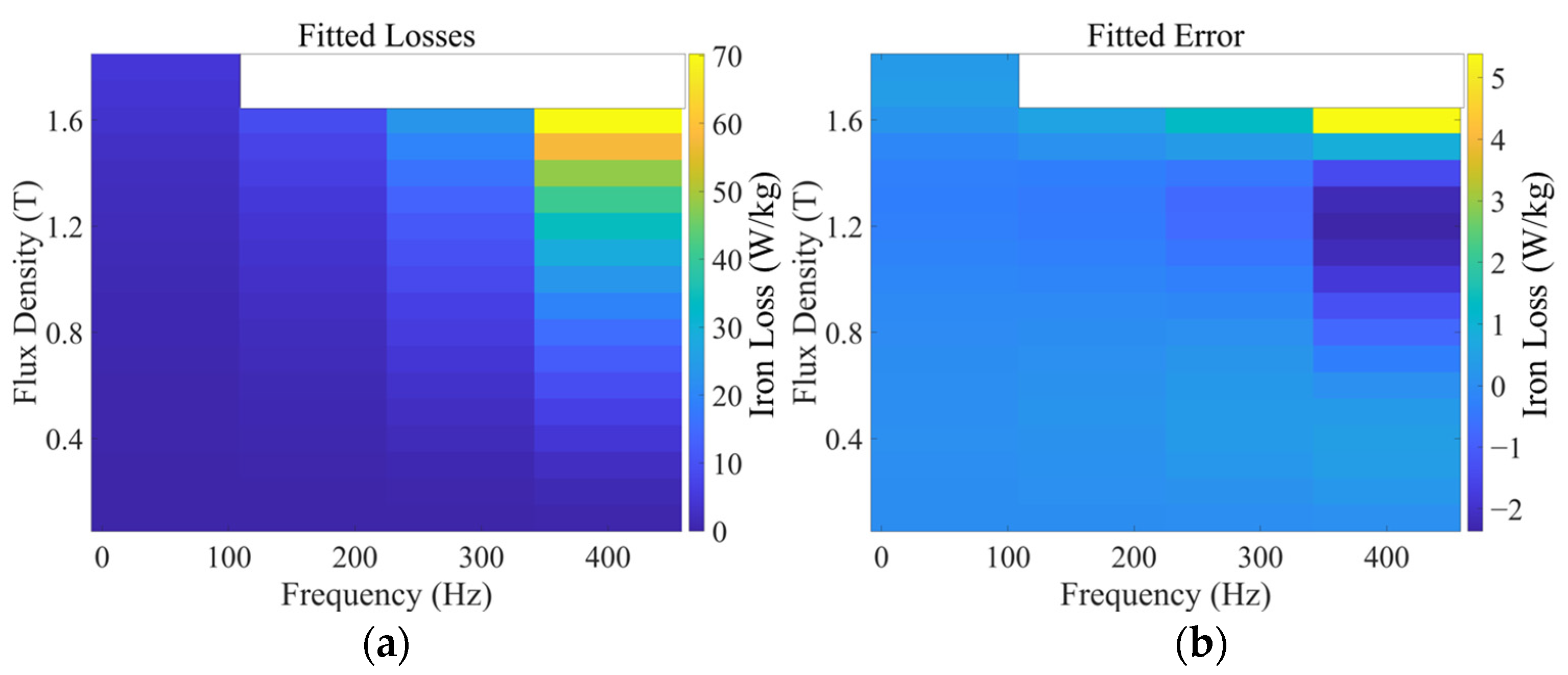
2.2. Polynomial Fitting Error

The traditional method of calculating iron loss necessitates measuring the loss value of the silicon steel sheet and then adjusting the coefficient of the iron loss calculation equation based on the empirical formula. However, when the motor is running at a high frequency, the coefficient fitting results based on the empirical formula will be significantly inaccurate. This does not meet the requirements of the iron loss calculation for high-speed motors. As Figure 2 shows, the calculated iron loss results and actual measurement results have a considerable discrepancy when the frequency and magnetic flux density increase [14,45]. The measurement of the iron loss of the motor can be calculated by:
p L o s s = p i n p c o p p e r p m e c h p o u t p s t r a y
There are two factors that can be used to determine the copper loss Pcopper: phase current and winding resistance. According to the method described in [46], the mechanical loss Pmech can be calculated from the output power and the stray loss can be calculated using the assumption stated in [47] that it represents 1% of the output power.
As is shown in Figure 3a, the fitting surface of the multi-frequency iron loss is presented. For each given flux density, as the frequency increases from 50 to 400 Hz, the iron loss generally increases. There is a positive correlation between frequency and iron loss. For each given frequency, as the flux density increases from 0.1 to 1.8, the iron loss generally increases. This also suggests a positive correlation between flux density and iron loss. The nonlinearity between iron loss, frequency, and flux density is evident in Figure 3b. As the frequency and magnetic flux density increase, the fitting relative error also rises, indicating a greater discrepancy between the actual value and the fitted results.
There is a possibility that the magnetic flux density waveform can be distorted due to the presence of high-order harmonics. Models that take into account the frequency and amplitude of the motor magnetic field, as well as the degree of distortion of the magnetic flux density waveform when calculating iron loss, can provide accurate information about the effect of the motor magnetic field frequency and amplitude on iron loss. By adding together the iron losses of the fundamental wave and all harmonic components, it is possible to determine the impact of harmonic flux density on motor iron loss. It is necessary to use radial and tangential magnetic flux density amplitudes instead of the ones in the traditional iron loss model in order to consider the effects of rotating magnetization on the magnetic flux density. It has been shown in Equation (2) that the iron loss expression with multifactor calculations includes compensation coefficients that are precise in determining how the frequency of a motor magnetic field, the amplitude of a magnetic flux density waveform distortion rate, and the distortion rate of a magnetic flux density waveform all affect the iron loss of a PMSM.
P L o s s = k t i = 0 6 n ± 1 [ k h ( f i , B i , B THD - r ) k h f 1 B 1 r α + k h ( f i , B i , B THD - t ) k h f 1 B 1 t α + k c ( f i , B i , B THD - r ) f 1 2 B 1 r α + k c ( f i , B i , B THD - t ) f 1 2 B 1 t α + k c ( f i , B i , B THD - r ) k e f 1 1.5 B 1 r 1.5 + k c ( f i , B i , B THD - t ) k e f 1 1.5 B 1 t α ]
where k t is the temperature coefficient k h ; k c , and k e represent the compensation coefficients; i is the order of the magnetic flux density harmonic i = 1 , 5 , 7 , 11 , 13 6 n ± 1 ( n = 1 , 2 , 3 ) ; f i is the i-th order frequency; B i is the amplitude of the i-th magnetic flux density harmonic; B i r and B i t are the amplitudes of magnetic flux density for the radial and tangential components of the i-th harmonic; and B THD - r and B THD - t are the magnetic flux density waveform distortion rates for the radial and tangential components, respectively.
The multifactor iron loss model in Equation (2) is reflected in Figure 4a, which displays the iron loss fitted result. As the frequency and flux density increase, the fit error also rises. Iron loss calculation results based on models depend on the precision of polynomial coefficient fitting and the lack of systematic evaluation criteria for the calculation results.

3. Iron Loss Estimation Based on the Recurrent Neural Network

To avoid the influence of the fitting coefficient, this study adopted the method based on PSO and an RNN to learn and train the relationship between input loss parameters and output iron loss, and establishes an estimation model of iron loss without relying on the empirical iron loss formula [48]. The logical structure of the system is shown in Figure 5, which mainly includes data acquisition, model training, result verification, and prediction. Using the PSO–RNN-based iron loss calculation method, all factors affecting iron loss are taken as input variables of the neural network, and the output result is the final iron loss result.

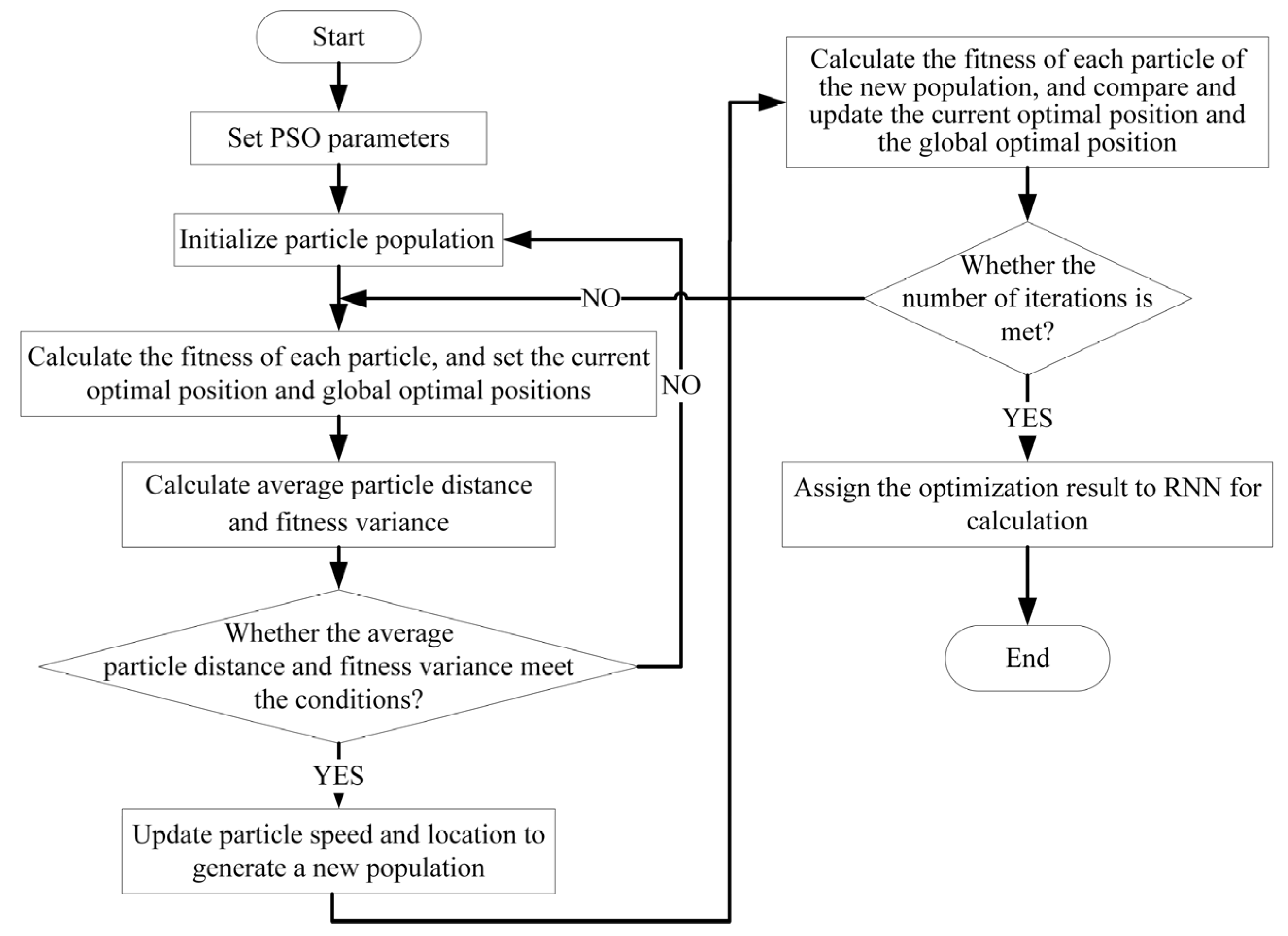
3.1. Particle Swarm Optimization and the Recurrent Neural Network

In PSO, the behavior of social groups is used as a basis for optimization. Several particles are involved in the algorithm, which is based on the search for the best possible solution in a multidimensional space. Throughout the iterative process, the particles adjust their positions as a result of their own experiences as well as the best solution that has been found by the collective swarm as a whole. PSO has been widely used in optimization tasks due to its simplicity and effectiveness in exploring solution spaces. It plays a significant role in finding optimal parameters for a diverse range of optimization problems, including applications in machine learning models and engineering designs. RNNs are a class of neural networks designed to process sequential data by maintaining internal memory or state. This enables them to capture temporal dependencies in data. Unlike traditional feedforward neural networks, RNNs possess loops that allow information to persist, making them suitable for tasks involving time series, natural language processing, and sequential data analysis.
In PSO, the optimal solution is determined by Gbest and Pbest. Gbest is referred to as the global best, while Pbest is the personal best. Every time, particles can be modified to identify the potential solution in terms of position and velocity vectors. Let V i and X i denote the velocity and position of the i-th particle. The velocity and position of each particle is then updated as [49]:
V i k + 1 = ω k V i k + C 1 r 1 ( P b e s t i k X i K ) + C 2 r 2 ( G b e s t i k X i K ) X i k + 1 = X i k + V i k + 1 ω k = ω min + ω max ω min 1 i t e r / i t e r max
The PSO algorithm involves the following steps: at each iteration k , the weight of the inertia ω k is calculated, the velocity of the i t h particle V i is determined, acceleration factors C 1 and C 2 are taken into account, uniform random numbers r 1 and r 2 in the range of [0,1] are generated, the best position of the i t h particle P b e s t i k and the best position of the group G b e s t i k are taken until iteration k is identified, the position of the i t h particle X i k is determined, the initial and final weights ω max and ω min are established, and the total number of iterations i t e r max is set. In order to understand how the convergence behavior of PSO can be influenced by the value of acceleration coefficients and inertia weights, the sensitivity of the convergence was studied by the authors in [50]. According to the findings of this research, it is possible to select the PSO parameters in a way that will guarantee convergence to an equilibrium state. Clerc and Kennedy [51] proposed various constriction models, and for each one, a specific constriction coefficient can be calculated to ensure convergence, depending on the chosen value of ϕ .
If the following criteria are met, then it should be possible to demonstrate that the path of a particle in an unconfined simplified PSO system with inertia will converge [51]:
1 > ω > 1 2 ( ϕ 1 + ϕ 2 ) 1 0
and 0 ω < 1 ; since ϕ 1 = c 1 U ( 0 , 1 ) and ϕ 2 = c 2 U ( 0 , 1 ) , the acceleration coefficients, c 1 and c 2 serve as upper bound of ϕ 1 and ϕ 2 . Equation (4) can be rewritten as:
1 > ω > 1 2 ( c 1 + c 2 ) 1 0
Hence, if ω , c 1 , and c 2 are chosen in a way that satisfies the condition in (5), the system is ensured to reach a steady state. Table 2 displays the parameters for the PSO algorithm.
Analysis of the PSO algorithm reveals that the PSO algorithm is capable of optimizing the weight of the RNN node. Typically, the connection weights of unoptimized RNNs are randomly set as initial values, which can result in issues such as slow training speed and convergence to local minima. Allocating space for the initial value in the PSO algorithm not only improves the model’s training speed, but also significantly lowers the risk of reaching the local optima.
Combining PSO and RNNs presents a robust and efficient approach to elevating RNN training and optimization processes. Leveraging PSO’s capabilities, this synergy optimizes various aspects of RNN architectures and parameters, exploring hyperparameter spaces effectively to enhance performance significantly beyond conventional methods. PSO assists in critical areas such as feature selection, weight initialization, and dynamic parameter adjustments, fostering faster convergence, improved generalization, and resilience against local optima during training. Moreover, the collaboration facilitates adaptive network design, refining RNN architectures to suit complex optimization landscapes by determining optimal layers, nodes, and connections. This integrated approach enhances RNN performance in tasks relying on accurate hyperparameters or architectural design. In addition, it accelerates convergence while fortifying models’ robustness and adaptability, demonstrating promising potential across diverse applications. The synergy between these methodologies aims to capitalize on the strengths of both techniques:
  • PSO will optimize the RNN architecture, hyperparameters, or training process to enhance the accuracy and efficiency of estimating iron loss.
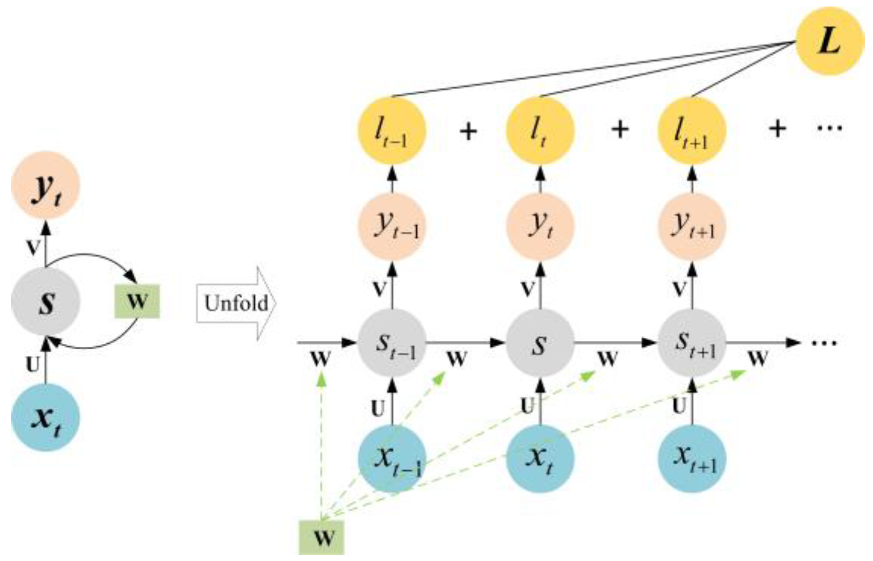
  • RNNs will serve as the predictive model, leveraging their ability to capture sequential dependencies in data for accurate estimation.
When comparing PSO to the whale algorithm and sparrow search algorithm for recurrent neural network optimization, PSO has certain advantages that might be considered superior in certain contexts, such as convergence speed and global exploration, simplicity and ease of implementation, parameter tuning and flexibility, and exploitation of the global best solution [52,53,54,55].
Figure 6 and Figure 7 show the optimization process of the PSO for RNN parameters and the RNN structure, respectively. The hidden layer in Figure 7 is represented by s, and the input and output layers by x and y, respectively. The weight matrix W is in the middle of the network, U represents the weight matrix between the input and hidden layers, V represents the weight matrix between hidden layers and output layers, and L represents the loss function. The model has the following structure formula:
s t = tanh ( U x t + W s t 1 ) y t = softmax ( V s t )
Table 3 lists the parameters of an RNN. For the input layer, the flux density, frequency, and temperature are the input variables. For the output layer, the iron loss estimation value is the output.

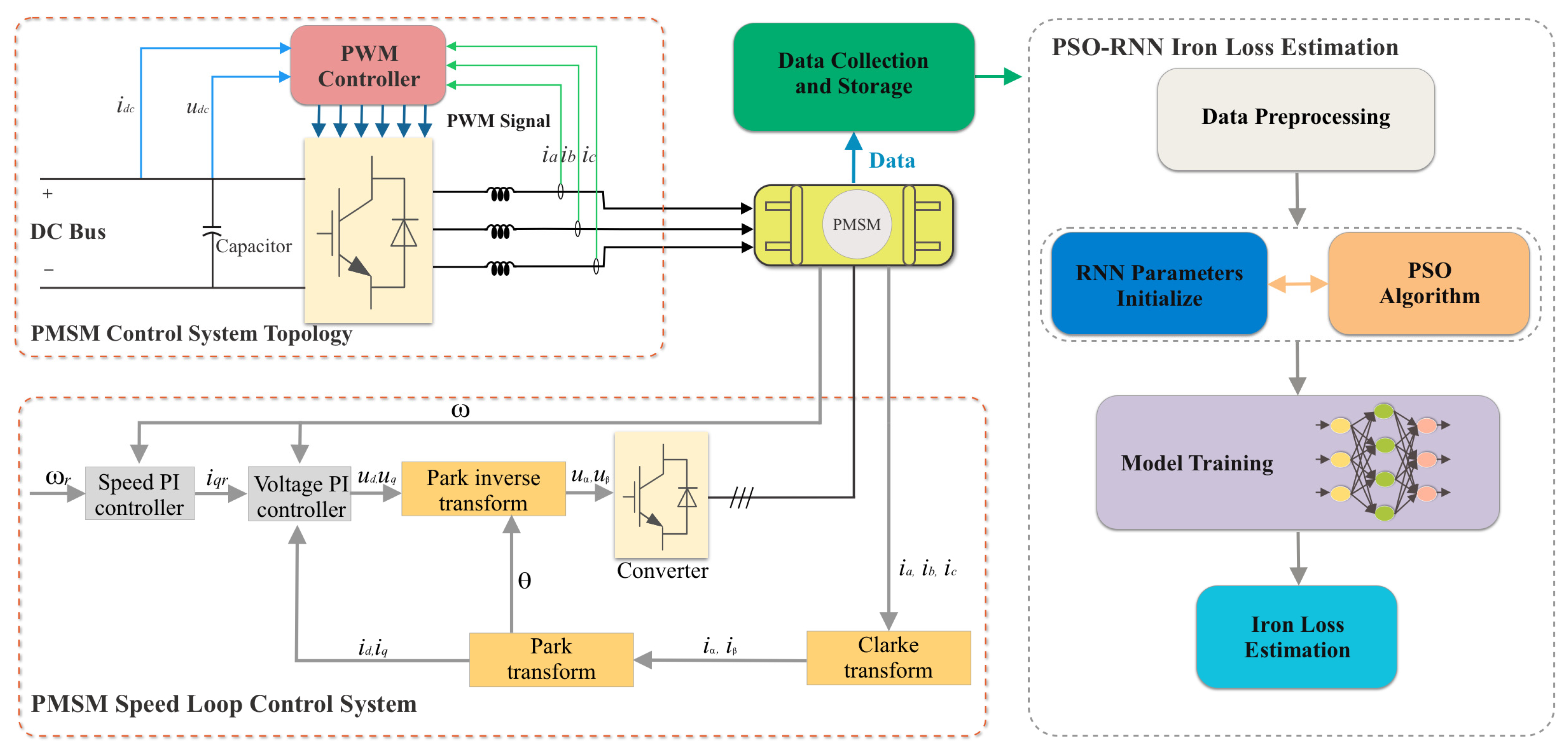
3.2. Proposed PMSM Iron Loss Method
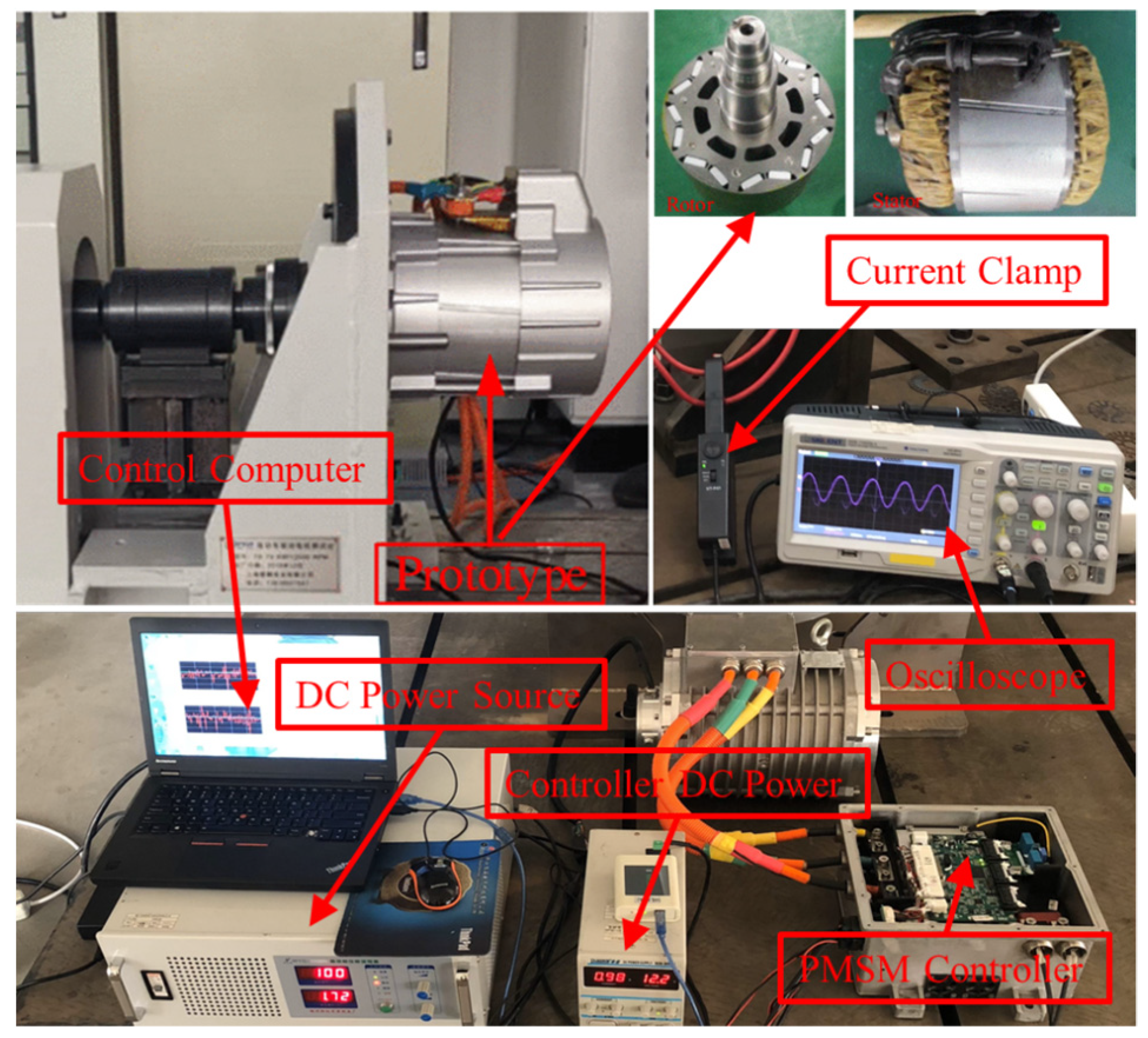
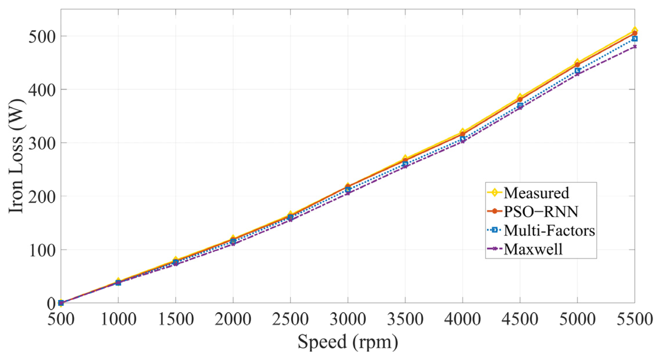
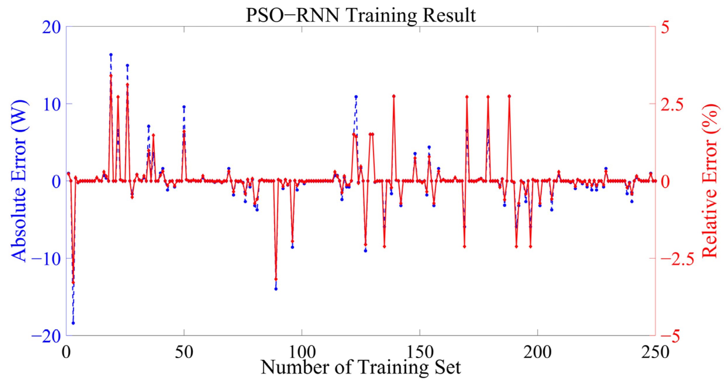
The PMSM control system combined with proposed PSO–RNN iron loss method is shown in Figure 8. Using the PSO–RNN-based iron loss calculation method, all factors affecting iron loss are taken as input variables of the neural network, and the output result is the final iron loss result. The RNN dataset is split into two subsets: training and validation sets. The training set is used to train the PSO–RNN model, where the model learns the patterns and relationships between input factors, magnetic flux densities, frequencies, temperatures, and iron loss. The validation set, on the other hand, is utilized to assess the model’s performance and generalizability after training. It helps evaluate how well the model can predict iron losses accurately on unseen data.
The split between the training and validation sets is crucial to ensure the model’s effectiveness and prevent overfitting. A representative validation dataset ensures that the model’s performance is evaluated across diverse scenarios, making the findings and predictions more reliable and applicable to real-world scenarios.

4. Result Analysis

On the basis of the above analysis, the interior PMSM has been selected in order to verify the proposed method. In Figure 9, a prototype of a PMSM combined with the hardware of the test bench for the experiment of the PMSM is presented. Table 4 contains the main parameters of the PMSM. A comparison of the calculated and measured values of iron loss is shown in Figure 10. According to the results of the study, the PSO–RNN-based calculation method has less error in the high-frequency part of the calculation as compared to the model-based calculation method. Using the training set of the iron loss model as a representative example, Figure 11 shows the absolute and relative errors of the model. The maximum relative error calculated by the PSO–RNN-based calculation model under different inputs is less than 3%, as demonstrated by the results.
Figure 12 displays the comparison between the predicted and measured values of the trained neural network model when different inputs are applied. The root mean square error (RMSE) is a metric that is widely used to evaluate the accuracy of predictions or estimates in comparison to the actual values in various fields, such as engineering, machine learning, and statistics. The formula for RMSE is:
R M S E = i = 1 n ( y ^ i y i ) 2 n
where y ^ 1 , y ^ 2 , , y ^ n are predicted values, y 1 , y 2 , y n are measured values, and n is the number of observations. For the iron loss prediction model, RMSE could be used to measure the average error between the estimated iron loss values by the model and the actual measured iron losses. A lower RMSE would indicate that the model’s predictions closely align with the observed iron losses, signifying better predictive accuracy. As is shown in Figure 12, the RNN RMSE between measured and estimated values is 1.3562, while the PSO–RNN RMSE between measured and estimated values is 0.1855. The results show that the trained calculation model can effectively predict iron loss under different inputs in large ranges.

5. Conclusions

This article presents a combined PSO–RNN approach to estimating the iron loss of a PMSM. The RNN was fed with multiple factors as the input parameters, and PSO was used to optimize the initial weights of the RNN. Based on the results of the proposed PSO–RNN method, it is evident that it can provide accurate estimates of iron loss over a wide range of inputs. As a result of calculating the maximum relative error by comparing the measured results with the estimated results for different inputs, the PSO–RNN model was able to achieve less than a 3% relative error.

6. Discussion

The combination of PSO and RNNs to estimate iron loss in PMSMs offers a promising avenue for enhancement. While the method exhibits strengths in accuracy and efficiency, it faces limitations such as data dependency, model interpretability challenges, and the complexity of parameter tuning. However, by extending this approach through hybrid modeling, feature selection, multi-objective optimization, adaptive strategies, additional data integration, and various other adaptations, the accuracy, efficiency, and applicability of iron loss estimation in diverse motor types can be significantly improved. These advancements hold potential for refining motor designs and fostering energy-efficient systems across industries.

Author Contributions

Conceptualization, K.X. and Y.G.; methodology, K.X., Y.G. and G.L.; software, K.X. and G.L.; validation, K.X., Y.G. and G.L.; formal analysis, J.Z. All authors have read and agreed to the published version of the manuscript.

Funding

This research was funded by China Scholarship Council (No. 202108140014).

Data Availability Statement

Data are contained within the article.

Conflicts of Interest

The authors declare no conflict of interest.

References

  1. Boubaker, N.; Matt, D.; Enrici, P.; Nierlich, F.; Durand, G. Measurements of iron loss in PMSM stator cores based on CoFe and SiFe lamination sheets and stemmed from different manufacturing processes. IEEE Trans. Magn. 2018, 55, 1–9. [Google Scholar] [CrossRef]
  2. Tong, W.; Sun, R.; Zhang, C.; Wu, S.; Tang, R. Loss and thermal analysis of a high-speed surface-mounted PMSM with amorphous metal stator core and titanium alloy rotor sleeve. IEEE Trans. Magn. 2019, 55, 1–4. [Google Scholar] [CrossRef]
  3. Zhang, C.; Guo, Q.; Li, L.; Wang, M.; Wang, T. System efficiency improvement for electric vehicles adopting a permanent magnet synchronous motor direct drive system. Energies 2017, 10, 2030. [Google Scholar] [CrossRef]
  4. Balamurali, A.; Kundu, A.; Li, Z.; Kar, N.C. Improved harmonic iron loss and stator current vector determination for maximum efficiency control of PMSM in EV applications. IEEE Trans. Ind. Appl. 2020, 57, 363–373. [Google Scholar] [CrossRef]
  5. Bertotti, G.; Boglietti, A.; Chiampi, M.; Chiarabaglio, D.; Fiorillo, F.; Lazzari, M. An improved estimation of iron losses in rotating electrical machines. IEEE Trans. Magn. 1991, 27, 5007–5009. [Google Scholar] [CrossRef]
  6. Lin, D.; Zhou, P.; Fu, W.; Badics, Z.; Cendes, Z. A dynamic core loss model for soft ferromagnetic and power ferrite materials in transient finite element analysis. IEEE Trans. Magn. 2004, 40, 1318–1321. [Google Scholar] [CrossRef]
  7. Steentjes, S.; Leßmann, M.; Hameyer, K. Advanced iron-loss calculation as a basis for efficiency improvement of electrical machines in automotive application. In Proceedings of the 2012 Electrical Systems for Aircraft, Railway and Ship Propulsion, Bologna, Italy, 16–18 October 2012; pp. 1–6. [Google Scholar]
  8. Fratila, M.; Benabou, A.; Tounzi, A.; Dessoude, M. Iron loss calculation in a synchronous generator using finite element analysis. IEEE Trans. Energy Convers. 2017, 32, 640–648. [Google Scholar] [CrossRef]
  9. Yamazaki, K.; Sato, Y.; Domenjoud, M.; Daniel, L. Iron loss analysis of permanent-magnet machines by considering hysteresis loops affected by multi-axial stress. IEEE Trans. Magn. 2019, 56, 1–4. [Google Scholar] [CrossRef]
  10. Abdi, S.; Abdi, E.; McMahon, R. A new iron loss model for brushless doubly-fed machines with hysteresis and field rotational losses. IEEE Trans. Energy Convers. 2021, 36, 3221–3230. [Google Scholar] [CrossRef]
  11. Huang, Y.; Dong, J.; Zhu, J.; Guo, Y. Core loss modeling for permanent-magnet motor based on flux variation locus and finite-element method. IEEE Trans. Magn. 2012, 48, 1023–1026. [Google Scholar] [CrossRef]
  12. Al-Timimy, A.; Giangrande, P.; Degano, M.; Galea, M.; Gerada, C. Investigation of ac copper and iron losses in high-speed high-power density PMSM. In Proceedings of the 2018 XIII International Conference on Electrical Machines (ICEM), Alexandroupoli, Greece, 3–6 September 2018; pp. 263–269. [Google Scholar]
  13. Liu, G.; Liu, M.; Zhang, Y.; Wang, H.; Gerada, C. High-speed permanent magnet synchronous motor iron loss calculation method considering multiphysics factors. IEEE Trans. Ind. Electron. 2019, 67, 5360–5368. [Google Scholar] [CrossRef]
  14. Liu, L.; Ba, X.; Guo, Y.; Lei, G.; Sun, X.; Zhu, J. Improved iron loss prediction models for interior PMSMs considering coupling effects of multiphysics factors. IEEE Trans. Transp. Electrif. 2022, 9, 416–427. [Google Scholar] [CrossRef]
  15. Yamazaki, K.; Watari, S. Loss analysis of permanent-magnet motor considering carrier harmonics of PWM inverter using combination of 2-D and 3-D finite-element method. IEEE Trans. Magn. 2005, 41, 1980–1983. [Google Scholar] [CrossRef]
  16. Yamazaki, K.; Abe, A. Loss analysis of interior permanent magnet motors considering carrier harmonics and magnet eddy currents using 3-D FEM. In Proceedings of the 2007 IEEE International Electric Machines & Drives Conference, Antalya, Turkey, 3–5 May 2007; Volume 2, pp. 904–909. [Google Scholar]
  17. Hwang, S.W.; Lim, M.S.; Hong, J.P. Hysteresis torque estimation method based on iron-loss analysis for permanent magnet synchronous motor. IEEE Trans. Magn. 2016, 52, 1–4. [Google Scholar] [CrossRef]
  18. Guo, Y.; Zhu, J.; Lu, H.; Li, Y.; Jin, J. Core loss computation in a permanent magnet transverse flux motor with rotating fluxes. IEEE Trans. Magn. 2014, 50, 1–4. [Google Scholar] [CrossRef]
  19. Denis, N.; Inoue, M.; Fujisaki, K.; Itabashi, H.; Yano, T. Iron loss reduction in permanent magnet synchronous motor by using stator core made of nanocrystalline magnetic material. IEEE Trans. Magn. 2017, 53, 1–6. [Google Scholar] [CrossRef]
  20. Zhu, S.; Dong, J.; Li, Y.; Hua, W. Fast calculation of carrier harmonic iron losses caused by pulse width modulation in interior permanent magnet synchronous motors. IET Electr. Power Appl. 2020, 14, 1163–1176. [Google Scholar] [CrossRef]
  21. Barcaro, M.; Bianchi, N.; Magnussen, F. Rotor flux-barrier geometry design to reduce stator iron losses in synchronous IPM motors under FW operations. IEEE Trans. Ind. Appl. 2010, 46, 1950–1958. [Google Scholar] [CrossRef]
  22. Arkadan, A.; Hijazi, T.; Masri, B. Design evaluation of conventional and toothless stator wind power axial-flux PM generator. IEEE Trans. Magn. 2017, 53, 1–4. [Google Scholar] [CrossRef]
  23. Guo, Y.; Zhu, J.G.; Lin, Z.W.; Zhong, J.J. 3D vector magnetic properties of soft magnetic composite material. J. Magn. Magn. Mater. 2006, 302, 511–516. [Google Scholar] [CrossRef]
  24. Huang, Z.; Fang, J.; Liu, X.; Han, B. Loss calculation and thermal analysis of rotors supported by active magnetic bearings for high-speed permanent-magnet electrical machines. IEEE Trans. Ind. Electron. 2015, 63, 2027–2035. [Google Scholar] [CrossRef]
  25. Popescu, M.; Ionel, D.M.; Boglietti, A.; Cavagnino, A.; Cossar, C.; McGilp, M.I. A general model for estimating the laminated steel losses under PWM voltage supply. IEEE Trans. Ind. Appl. 2010, 46, 1389–1396. [Google Scholar] [CrossRef]
  26. Zhang, D.; Liu, T.; Zhao, H.; Wu, T. An analytical iron loss calculation model of inverter-fed induction motors considering supply and slot harmonics. IEEE Trans. Ind. Electron. 2019, 66, 9194–9204. [Google Scholar] [CrossRef]
  27. Popescu, M.; Ionel, D.M. A best-fit model of power losses in cold rolled-motor lamination steel operating in a wide range of frequency and magnetization. IEEE Trans. Magn. 2007, 43, 1753–1756. [Google Scholar] [CrossRef]
  28. Bi, L.; Schäfer, U.; Hu, Y. A new high-frequency iron loss model including additional iron losses due to punching and burrs’ connection. IEEE Trans. Magn. 2020, 56, 1–9. [Google Scholar] [CrossRef]
  29. Ionel, D.M.; Popescu, M.; Dellinger, S.J.; Miller, T.; Heideman, R.J.; McGilp, M.I. On the variation with flux and frequency of the core loss coefficients in electrical machines. IEEE Trans. Ind. Appl. 2006, 42, 658–667. [Google Scholar] [CrossRef]
  30. Jia, W.; Xiao, L.; Zhu, D.; Wei, J. An improved core-loss calculation method with variable coefficients based on equivalent frequency. IEEE Trans. Magn. 2018, 54, 1–5. [Google Scholar]
  31. Chen, J.; Wang, D.; Jiang, Y.; Teng, X.; Cheng, S.; Hu, J. Examination of temperature-dependent iron loss models using a stator core. IEEE Trans. Magn. 2018, 54, 1–7. [Google Scholar] [CrossRef]
  32. Seo, K.S.; Kim, H.D.; Lee, K.H.; Park, I.H. Numerical and experimental characterization of thread-type magnetic core with low eddy current loss. IEEE Trans. Magn. 2015, 51, 1–4. [Google Scholar] [CrossRef]
  33. Han, S.H.; Jahns, T.M.; Zhu, Z.Q. Analysis of rotor core eddy-current losses in interior permanent-magnet synchronous machines. IEEE Trans. Ind. Appl. 2009, 46, 196–205. [Google Scholar] [CrossRef]
  34. Wang, Y.; Ma, J.; Liu, C.; Lei, G.; Guo, Y.; Zhu, J. Reduction of magnet eddy current loss in PMSM by using partial magnet segment method. IEEE Trans. Magn. 2019, 55, 1–5. [Google Scholar] [CrossRef]
  35. Steentjes, S.; von Pfingsten, G.; Hombitzer, M.; Hameyer, K. Iron-loss model with consideration of minor loops applied to FE-simulations of electrical machines. IEEE Trans. Magn. 2013, 49, 3945–3948. [Google Scholar] [CrossRef]
  36. Ruuskanen, V.; Nerg, J.; Rilla, M.; Pyrhönen, J. Iron loss analysis of the permanent-magnet synchronous machine based on finite-element analysis over the electrical vehicle drive cycle. IEEE Trans. Ind. Electron. 2016, 63, 4129–4136. [Google Scholar] [CrossRef]
  37. Marracci, M.; Tellini, B. Hysteresis losses of minor loops versus temperature in MnZn ferrite. IEEE Trans. Magn. 2012, 49, 2865–2869. [Google Scholar] [CrossRef]
  38. Shimizu, K.; Furuya, A.; Uehara, Y.; Fujisaki, J.; Kawano, H.; Tanaka, T.; Ataka, T.; Oshima, H. Loss simulation by finite-element magnetic field analysis considering dielectric effect and magnetic hysteresis in EI-Shaped Mn–Zn ferrite core. IEEE Trans. Magn. 2018, 54, 1–5. [Google Scholar] [CrossRef]
  39. Krings, A.; Soulard, J. Overview and comparison of iron loss models for electrical machines. J. Electr. Eng. 2010, 10, 8. [Google Scholar]
  40. Jing, Y.; Zhang, Y.; Zhu, J. Iron Loss Calculation of High Frequency Transformer Based on A Neural Network Dynamic Hysteresis Model. In Proceedings of the 2022 IEEE 20th Biennial Conference on Electromagnetic Field Computation (CEFC), Denver, CO, USA, 24–26 October 2022; pp. 1–2. [Google Scholar] [CrossRef]
  41. Reljić, D.D.; Matić, D.Z.; Jerkan, D.G.; Oros, D.V.; Vasić, V.V. The estimation of iron losses in a non-oriented electrical steel sheet based on the artificial neural network and the genetic algorithm approaches. In Proceedings of the 2014 IEEE International Energy Conference (ENERGYCON), Cavtat, Croatia, 13–16 May 2014; pp. 51–57. [Google Scholar] [CrossRef]
  42. Truong, P.H.; Flieller, D.; Nguyen, N.K.; Mercklé, J.; Dat, M.T. Optimal efficiency control of synchronous reluctance motors-based ANN considering cross magnetic saturation and iron losses. In Proceedings of the IECON 2015—41st Annual Conference of the IEEE Industrial Electronics Society, Yokohama, Japan, 9–12 November 2015; pp. 004690–004695. [Google Scholar] [CrossRef]
  43. Baosteel, B. Cold-Rolled Non-Oriented Electrical Steel. 2023. Available online: https://ecommerce.ibaosteel.com/portal/download/manual/NGO.pdf (accessed on 27 November 2023).
  44. Baosteel, B. Baosteel Products Electrical Steel. 2023. Available online: http://esales.baosteel.com/baosteel_products/eleSteel/en/products/products_04_2.jsp (accessed on 25 November 2023).
  45. Sun, X.; Shi, Z.; Lei, G.; Guo, Y.; Zhu, J. Multi-objective design optimization of an IPMSM based on multilevel strategy. IEEE Trans. Ind. Electron. 2020, 68, 139–148. [Google Scholar] [CrossRef]
  46. Guo, Y.; Zhu, J.; Lu, H.; Lin, Z.; Li, Y. Core loss calculation for soft magnetic composite electrical machines. IEEE Trans. Magn. 2012, 48, 3112–3115. [Google Scholar] [CrossRef]
  47. Lei, G.; Zhu, J.; Guo, Y. Multidisciplinary Design Optimization Methods for Electrical Machines and Drive Systems; Springer: Berlin/Heidelberg, Germany, 2016; Volume 691. [Google Scholar]
  48. Xu, K.; Guo, Y.; Lei, G.; Liu, L.; Zhu, J. Calculation of Iron Loss in Permanent Magnet Synchronous Motors Based on PSO-RNN. In Proceedings of the 2023 IEEE International Magnetic Conference-Short Papers (INTERMAG Short Papers), Sendai, Japan, 15–19 May 2023; pp. 1–2. [Google Scholar]
  49. Xu, K.; Guo, X.H.; Dai, J.Q.; Du, S.F.; Wang, Z.X.; Wang, Q.X. An Improved PSO for SHEPWM Applied to Three-Level Topology-based PMSM Driver System. J. Comput. 2019, 30, 195–206. [Google Scholar]
  50. Clerc, M.; Kennedy, J. The particle swarm-explosion, stability, and convergence in a multidimensional complex space. IEEE Trans. Evol. Comput. 2002, 6, 58–73. [Google Scholar] [CrossRef]
  51. Van den Bergh, F.; Engelbrecht, A.P. A study of particle swarm optimization particle trajectories. Inf. Sci. 2006, 176, 937–971. [Google Scholar] [CrossRef]
  52. Singh, L.; Dutta, N. Various Optimization algorithm used in CRN. In Proceedings of the 2020 International Conference on Computation, Automation and Knowledge Management (ICCAKM), Dubai, United Arab Emirates, 9–10 January 2020; pp. 95–100. [Google Scholar]
  53. Shami, T.M.; El-Saleh, A.A.; Alswaitti, M.; Al-Tashi, Q.; Summakieh, M.A.; Mirjalili, S. Particle swarm optimization: A comprehensive survey. IEEE Access 2022, 10, 10031–10061. [Google Scholar] [CrossRef]
  54. Gharehchopogh, F.S.; Namazi, M.; Ebrahimi, L.; Abdollahzadeh, B. Advances in sparrow search algorithm: A comprehensive survey. Arch. Comput. Methods Eng. 2023, 30, 427–455. [Google Scholar] [CrossRef] [PubMed]
  55. Rana, N.; Latiff, M.S.A.; Abdulhamid, S.M.; Chiroma, H. Whale optimization algorithm: A systematic review of contemporary applications, modifications and developments. Neural Comput. Appl. 2020, 32, 16245–16277. [Google Scholar] [CrossRef]
Figure 1. Loss curves of silicon steel sheet with different temperatures at (a) 50 Hz and (b) 200 Hz.
Magnetism 03 00025 g001
Figure 2. Multi-frequency iron loss fitting curve.
Magnetism 03 00025 g002
Figure 3. Multi-frequency iron loss fitting results: (a) fitting surface and (b) fitting relative error.
Magnetism 03 00025 g003aMagnetism 03 00025 g003b
Figure 4. Multi-frequency iron loss: (a) Fitting results and (b) error distribution.
Magnetism 03 00025 g004
Figure 5. Logical diagram of the proposed system.
Magnetism 03 00025 g005
Figure 6. RNN parameter optimization process by PSO.
Magnetism 03 00025 g006
Figure 7. RNN structure.
Magnetism 03 00025 g007
Figure 8. PMSM control system combined with proposed PSO–RNN iron loss method.
Magnetism 03 00025 g008
Figure 9. The prototype of PMSM and hardware of test bench.
Magnetism 03 00025 g009
Figure 10. Iron loss calculation results of different methods.
Magnetism 03 00025 g010
Figure 11. Absolute and relative errors of training set.
Magnetism 03 00025 g011
Figure 12. Comparison between the predicted and the measured values: (a) original RNN and (b) PSO–RNN.
Magnetism 03 00025 g012
Table 1. Classic iron loss models.
Loss Model NameExpressionNo. of Parameters
Steinmetz [39] P s t m = k h f n B m 3
Steinmetz with eddy
current loss
P i s t m = k h f n B m + k c ( f B ) 2 4
Bertotti [5] P B e r = k h f B α + k c ( f B ) 2 + k e ( f B ) 1.5 4
ANSYS Maxwell [6] P Maxwell   = k h f B 2 + k c ( f B ) 2 + k e ( f B ) 1.5 3
Improved loss model [7] P i m p = α 1 k 1 f B α + α 2 ( f B ) 2 + α 2 α 3 f 2 B α 4 + 2 + α 5 k 2 ( f B ) 1.5 5
Table 2. Parameters of the PSO algorithm.
NameValue
Population size100
Acceleration constant C1 and C21.4
Inertia weight ω max 0.9
Inertia weight ω min 0.4
Particle dimension1
Maximum number of iterations30
Table 3. Parameters of RNN.
NameValue
Dimension of hidden layer13
Dimension of output layer1
Dimension of input layer1
Number of recurrent layers3
Number of features in the hidden state6
Number of input sizes3
Table 4. Parameters of the PMSM.
NameUnitValue
Stator outer radiusmm196
Rotor outer radiusmm134
Core lengthmm108
Airgap lengthmm0.5
Number of poles-8
Number of slots-48
Rated powerkW20
Rated torqueNm53
Rated speedrpm3600
PM Material-NdFeB-35
Core material-35WW360
Maximum speedrpm5500
Disclaimer/Publisher’s Note: The statements, opinions and data contained in all publications are solely those of the individual author(s) and contributor(s) and not of MDPI and/or the editor(s). MDPI and/or the editor(s) disclaim responsibility for any injury to people or property resulting from any ideas, methods, instructions or products referred to in the content.

