Analytical Modelling of the Slot Opening Function

Abstract

The slot opening function, also called relative air gap permeance, is a function which, multiplied by the flux density distribution of a slotless geometry, gives the flux density distribution of a slotted configuration. Here, the magnetic field inside the air gap of a multi-slot surface facing a smooth one was studied, by solving the Laplace equation inside the air gap, in terms of a Fourier series. To obtain the Fourier coefficients, at first, the conformal mapping analytical solution of a single-slot configuration along the smooth surface, was considered. Then, the principle of superposition of the single-slot lost flux density distributions was applied to obtain the multi-slot distribution. The approach is valid in general, and in the case of interference among the flux density distributions of adjacent slots, where their mutual effect cannot be neglected. The field distributions obtained by using the proposed slot opening functions were compared with FEM simulations, showing satisfactory agreement. The numerical accuracy limits were also analysed and discussed.

1. Introduction

A precise estimation of the air gap field inside electrical machines is really important in order to properly estimate local and integral quantities and thus predict machine performance. Most of the methods used in the literature start with the study of the air gap field between smooth ferromagnetic surfaces (slotless approach) [1,2,3,4,5,6] and subsequently, the effect on the field due to the presence of slotting is introduced, making use of a slotting function which can also be called the air gap relative permeance function.

The air gap relative permeance function was initially introduced by [7,8] using magnetic circuit theories. Magnetomotive force (m.m.f.) and the concept of permeance were used together with conformal mapping in order to retrieve the aforementioned function, which was developed only for a normal flux density component. Making use of a similar approach, Ref. [9] also studied the behaviour of the tangential component introducing the concept of a complex relative permeability function, useful for calculating quantities like the cogging torque throughout the integration of the Maxwell stress tensor [10]. Other topologies of the slot opening function were later developed solving the Laplace equations inside the air gap in terms of Fourier series, by assuming the flux density distributions in some region of it, in particular, using approximate functions [11,12,13]. However, most of the approaches present in the literature that refer to these methods, describing the slot opening function, do not consider the effect of adjacent slots [11,12,13,14,15,16], which, in certain circumstances, cannot be neglected. Inside the following work, a procedure to retrieve the slotting function will be introduced, also considering the effects of adjacent slots.

The air gap field of a slotted surface facing a smooth one has been studied for a few decades: the first, classical analysis was based on a conformal mapping method, as developed by Carter, by solving the Schwarz–Christoffel equation [17,18].

The air gap relative permeance function was introduced in [9], where the air gap flux density distribution was obtained by numerically inverting the conformal mapping solution in the complex domain. However, this analysis, as it has already been pointed out previously, did not consider the presence of adjacent slots, being based on a single-slot approach. Thus, it is only sufficiently accurate if the single-slot flux density distributions of adjacent slots do not interfere with each other; this occurs if the equivalent air gap g is “small” compared to the slot opening b_s and the slot pitch τ_s, for example, in induction machines. However, when the equivalent air gap g is not “small” anymore compared to the slot opening b_s and the slot pitch τ_s, the precision of the method gets degraded, due to the effect of adjacent slots being stronger and not negligible anymore.

The approach adopted here is based on the field solution of the Laplace equation in the air gap, for a multi-slot disposition, expressed in terms of Fourier series. To obtain the Fourier coefficients, at first, the single-slot field analytical solution was considered, along a smooth surface, as obtained in [18]. As for the multi-slot disposition, the calculation was based on the principle of superposition of the lost flux density distribution of each slot. This made the result correct also in the case of a “high” magnetic air gap width, for example, if the machine is a surface mounted permanent magnet (SPM) synchronous machine.

The paper consists of the following: in Section 2, the formulation of the Laplace equation in the air gap is outlined for a multi-slot disposition, and the symmetry and periodicity field properties are analysed; in Section 3, the single-slot air gap field was studied by conformal transformation, and the normal component of the flux density distribution along the smooth surface was obtained; in Section 4, the single-slot lost flux density function is introduced and its distribution was superimposed with those of the other slots, from which the multi-slot opening function was obtained, along the smooth surface; in Section 5, the integrals for the Fourier coefficient calculation, written for a multi-slot disposition, are reformulated in terms of single-slot Fourier integrals; Section 6 shows how the slotting function can be expressed in complex form; in Section 7, a few slot opening function distributions are plotted, for different geometric parameters (with “high” and “small” air gap widths) and for different exploration lines in the air gap, comparing the results with FEM simulations; Section 8 discusses some numerical convergence and accuracy limits; and in Section 9, some conclusions and perspectives are drawn.

In all the diagrams illustrated in the following sections, the units of the variables along the axes are omitted, because they are all expressed as pu quantities.

2. Laplace Equation for a Multi-Slot Disposition: Solution Structure and Properties

Figure 1 shows the considered air gap geometry, the main dimensions and the reference frame adopted for the analysis of the magnetic field in a slotted air gap.

Let us consider a multi-slot upper surface facing a smooth lower one, where τ_s is the slot pitch; for this situation, the adopted reference frame xy is centred at the point c.

In the air gap, the magnetic field is described by the vector potential component A(x, y), perpendicular to the xy plane, as the solution to the Laplace equation:

$$\frac{{\partial }^{2}A}{\partial x^2}+\frac{{\partial }^{2}A}{\partial y^2}=0.$$

(1)

The generic point (x, y) inside the air gap can also be defined by using a complex variable z that in the xy reference frame of Figure 1 can be written as the following: z = x + j·y.

By adopting the method of separation of the variables, A(x, y) can be written in terms of a series, according to the following expression:

$$A\left(x,y\right)=-B_o\cdot x+{\displaystyle \sum _{k=1}^{\infty }{A}_k\cdot \cosh \left(k\cdot 2\pi \cdot y/{\tau }_s\right)}\cdot \sin \left(k\cdot 2\pi \cdot x/{\tau }_s\right).$$

(2)

It is easy to verify that (2) satisfies (1).

Considering that the x and y flux density components are given by

$$\{\begin{array}{l}{B}_x\left(x,y\right)=+\partial A\left(x,y\right)/\partial y\\ B_y\left(x,y\right)=-\partial A\left(x,y\right)/\partial x\end{array},$$

(3)

from (2), we obtain

$$\{\begin{array}{l}{B}_x\left(x,y\right)={\displaystyle \sum _{k=1}^{\infty }{B}_k\cdot \sinh \left(k\cdot 2\pi \cdot y/{\tau }_s\right)}\cdot \sin \left(k\cdot 2\pi \cdot x/{\tau }_s\right)\\ B_y\left(x,y\right)=B_o-{\displaystyle \sum _{k=1}^{\infty }{B}_k\cdot \cosh \left(k\cdot 2\pi \cdot y/{\tau }_s\right)}\cdot \cos \left(k\cdot 2\pi \cdot x/{\tau }_s\right)\end{array},$$

(4)

with

$$B_k=k\cdot \left(2\pi /{\tau }_s\right)\cdot A_k.$$

(5)

In (2) and in (4), B_o is the average flux density, calculated within the slot pitch τ_s:

$$B_o=\frac{1}{{\tau }_s}\cdot {\displaystyle {\int }_{-{\tau }_s/2}^{{\tau }_s/2}{B}_y\left(x,y\right)\cdot dx}.$$

(6)

while the B_y(x,y) distribution shape depends on the position y chosen for the horizontal exploration line in the air gap, it is possible to show that B_o does not depend on y.

If the upper surface would have been smooth like the lower one, the flux density in the air gap would possess just the y component which would be uniform; referring to it as the ideal flux density B_i, its value can be calculated as

$$B_i={\mu }_o\cdot U/g,$$

(7)

where U is the magnetic voltage drop across the two surfaces.

If we divide the air gap flux density components in (4) by B_i, the pu flux density components β_x and β_y can be written as

$$\{\begin{array}{l}{\beta }_x\left(x,y\right)=\frac{B_x\left(x,y\right)}{B_i}={\displaystyle \sum _{k=1}^{\infty }{\beta }_k\cdot \sinh \left(k\cdot 2\pi \cdot y/{\tau }_s\right)}\cdot \sin \left(k\cdot 2\pi \cdot x/{\tau }_s\right)\\ {\beta }_y\left(x,y\right)=\frac{B_y\left(x,y\right)}{B_i}={\beta }_o-{\displaystyle \sum _{k=1}^{\infty }{\beta }_k\cdot \cosh \left(k\cdot 2\pi \cdot y/{\tau }_s\right)}\cdot \cos \left(k\cdot 2\pi \cdot x/{\tau }_s\right)\end{array}.$$

(8)

with

$${\beta }_k=B_k/B_i.$$

(9)

and

$${\beta }_o=B_o/B_i=1/K_C,$$

(10)

where K_C is the Carter’s factor [17]

$$K_C=\frac{1}{1-{\sigma }_s\cdot \left(b_s/{\tau }_s\right)},\mathrm{with}{\sigma }_s=\frac{2}{\pi }\cdot \left\{\mathrm{atan}\left(\frac{1}{2}\cdot \frac{b_s}{g}\right)-\frac{g}{b_s}\cdot \ln \left[1+{\left(\frac{1}{2}\cdot \frac{b_s}{g}\right)}^2\right]\right\}.$$

(11)

From the inspection of (8), the following properties can be recognized, for any value of y (0 ≤ y ≤ g). Of course, the same properties are also valid also for (4):

-

Equation (8) is periodic in space, along the x axis, with a period equal to the slot pitch τ_s:

$$\{\begin{array}{l}{\beta }_x\left(x,y\right)={\beta }_x\left(x+h\cdot {\tau }_s,y\right)\\ {\beta }_y\left(x,y\right)={\beta }_y\left(x+h\cdot {\tau }_s,y\right)\end{array}\hspace{1em}\hspace{1em}h=\pm 1,\pm 2,\dots ;$$

(12)

-

The functions β_x and β_y are symmetrical with respect to the origin O of the xy reference frame:

$$\{\begin{array}{l}{\beta }_x\left(+x,y\right)=-{\beta }_x\left(-x,y\right)\\ {\beta }_y\left(+x,y\right)={\beta }_y\left(-x,y\right)\end{array}.$$

(13)

-

For x = ±τ_s/2, the β_x component is zero:

$${\beta }_x\left(\pm {\tau }_s/2,y\right)=0.$$

(14)

Thus, the solution of (1) was reduced to calculate the coefficients β_k (or Ak, from (5) and (9)), for k = 1, 2… ∞. In practice, the series should be extended up to a maximum suited term k_M, as will be discussed later.

3. Single-Slot Air Gap Field Analysis by Conformal Transformation

In order to calculate the coefficients β_k, at first, the field of the single-slot system must be studied using conformal transformations [18], as resumed in this section.

Figure 2 shows the single-slot disposition, with the same air gap and slot opening dimensions considered in Figure 1.

Here, in order to apply the conformal transformation procedure, a corner of the Schwarz–Christoffel polygon should be chosen as the origin of the plane; thus, the corner b of Figure 2 was chosen as the origin of the reference frame x_by_b. The new complex position variable was z_b = x_b + j·y_b.

By writing the Schwarz–Christoffel equation, the transformation from the z_b plane (z_b = x_b + j·y_b) to the w plane (w = u + j·v) is represented by the following equation [18]:

$$\frac{d{\mathit{z}}_b}{d\mathit{w}}=\frac{g}{\pi }\cdot \frac{\sqrt{\mathit{w}-a}\cdot \sqrt{\mathit{w}-b}}{\mathit{w}\cdot \left(\mathit{w}-1\right)},$$

(15)

where

$$b={\left[\frac{b_s}{2\cdot g}+\sqrt{\frac{{\left(b_s/g\right)}^2+4}{2}}\right]}^2,a=1/b.$$

(16)

Then, by integrating (15), the function z_b(w) was retrieved as

$${\mathit{z}}_b\left(\mathit{w}\right)=\frac{g}{\pi }\cdot \left\{\ln \left[\frac{1+p\left(\mathit{w}\right)}{1-p\left(\mathit{w}\right)}\right]-\ln \left[\frac{b+p\left(\mathit{w}\right)}{b-p\left(\mathit{w}\right)}\right]-2\cdot \frac{b-1}{\sqrt{b}}\cdot \mathrm{atan}\left[\frac{p\left(\mathit{w}\right)}{\sqrt{b}}\right]\right\},$$

(17)

with

$$p\left(\mathit{w}\right)=\sqrt{\left(\mathit{w}-b\right)/\left(\mathit{w}-a\right)}.$$

(18)

As regards the flux density vector in the air gap, for a single-slot configuration (subscript s), referred to the ideal flux density B_i, the following expression was obtained, as a function of the complex variable w [18]:

$${\mathit{\beta }}_s\left(\mathit{w}\right)={\mathit{B}}_s\left(\mathit{w}\right)/B_i=\frac{\mathit{w}-1}{\sqrt{\mathit{w}-a}\cdot \sqrt{\mathit{w}-b}},$$

(19)

from which the x_b and y_b components followed as

$${\beta }_{sx}\left(\mathit{w}\right)=\mathrm{Re}\left[{\mathit{\beta }}_s\left(\mathit{w}\right)\right],{\beta }_{sy}\left(\mathit{w}\right)=\mathrm{Im}\left[{\mathit{\beta }}_s\left(\mathit{w}\right)\right].$$

(20)

In principle, the elimination of the variable w in putting together (17) and (20) would give the slotting opening functions β_sx(z_b) and β_sy(z_b) for the single-slot disposition but unfortunately, (17) could not be inverted in closed form.

Moreover, if a generic position z_b = x_b + j·y_b was considered inside the air gap (with x_b as the exploring variable and y_b < g kept constant during exploration), the numerical inversion of (18) in the complex domain, as described in [9], exhibited some convergence issues.

An alternative approach to obtain the Fourier series coefficients β_k of (8) is described in [12]. It is based on an approximated formulation of the field along the slot opening segment; however, the accuracy of the obtained distributions could be critical, depending on the air gap geometry and on the exploring line position in the air gap.

4. Single-Slot and Multi-Slot Normal Slotting Function along a Smooth Surface

The numerical inversion of (17) was easier along the smooth surface (where y_b = g), because the calculation involved just real variables (x_b and u); in fact, along the smooth surface, where we had z_b = x_b + j·g, w = u occurred.

Due to the slotting function symmetry with respect to the slot axis, the interval of interest for x_b was −b_s/2 ≤ x_b < ∞, corresponding to −1 ≥ u > −∞ for w = u (see Figure 2); in practice, u_lim = 1013 can be adopted, from which, by (17), it follows that x_lim = Re[z_b(−u_lim)].

For example, with g = 5 mm, b_s = 5 mm, τ_s = 10 mm, we obtained x_lim = 45.5 mm = 4.55·τ_s.

For any sampling point x_b + j·g along the smooth surface in the interval −b_s/2 ≤ x_b < x_lim, the numerical inversion of (17) gives the corresponding w values:

$$\mathit{w}\left(x_b\right)=root\left[{\mathit{z}}_b\left(w_g\right)-\left(x_b+j\cdot g\right),w_g\right],$$

(21)

where the function “root” looks for the zero condition of the first argument inside square brackets and w_g is a guess value, here set to −1, corresponding to the point c present in Figure 1.

To ensure suitably accurate results from (21), the convergence tolerance, TOL, should be set to the smallest value compatible with a stable numerical solution (here TOL = 10⁻¹⁵).

Coming back to the xy reference frame shown in Figure 1, by applying a displacement equal to b_s/2, and considering the 2nd of (13), it follows that

$$u\left(x\right)=w\left(\left|x_b-b_s/2\right|\right),v=0.$$

(22)

Thus, from (19), the normal component β_sy0(x) of the single-slot slotting function along the smooth surface (subscript 0, because y = 0) can be written as the following:

$${\beta }_{sy0}\left(x\right)=\frac{u\left(x\right)-1}{\sqrt{u\left(x\right)-a}\cdot \sqrt{u\left(x\right)-b}}.$$

(23)

The single-slot slotting function of the slot positioned h slot pitches at the left of the original one could be easily obtained by displacing the slotting function (23): β_sy0(x − h·τ_s). Of course, if h was negative, the displaced slot was positioned at the right of the original one.

Figure 3 shows the single-slot slotting functions β_sy0(x − h·τ_s) with h = −2, −1, 0, 1, 2, again for g = 5 mm, b_s = 5 mm, τ_s = 10 mm.

For h = 0, the analytical curve is shown together with the FEM curve [19], with bold lines.

For x/τ_s = ±0.5, β_sy0(±τ_s/2) appears significantly lower than 1. This means that the single-slot slotting functions of adjacent slots interfered among each other; in this situation, the air gap width could be qualified as “high”.

The complement to 1 of the single-slot slotting function can be called the single-slot lost flux density function; for the central slot we can write

$${\beta }_{\ell sy0}\left(x\right)=1-{\beta }_{sy0}\left(x\right),$$

(24)

and for a generic slot positioned h slots at the left of the central one:

$${\beta }_{\ell hy0}\left(x\right)={\beta }_{\ell sy0}\left(x-h\cdot {\tau }_s\right)\hspace{1em}\hspace{1em}h=\pm 1,\pm 2,\dots .$$

(25)

In the case of a multi-slot configuration, the total lost flux density function β_ℓy0(x) can be expressed as the following:

$${\beta }_{\ell y0}\left(x\right)={\displaystyle \sum _{h=-\infty }^{\infty }{\beta }_{\ell sy0}\left(x-h\cdot {\tau }_s\right)}.$$

(26)

Equation (26) corresponds to the formulation of the so-called principle of superposition of the distributions of the single-slot lost flux density functions: the lost flux density along a smooth structure, due to an infinite number of slots in the faced structure, can be expressed by means of a sequence of single-slot flux density distributions, separately evaluated for every slot as if they would be present on their own. This principle is valid even in the case that the lost flux density curves of adjacent slots interfere among them.

Finally, the multi-slot slotting function β_y0(x) is given by the following:

$${\beta }_{y0}\left(x\right)=1-{\beta }_{\ell y0}\left(x\right)=1-{\displaystyle \sum _{h=-\infty }^{\infty }{\beta }_{\ell sy0}\left(x-h\cdot {\tau }_s\right)}.$$

(27)

Figure 4 shows the distribution of the multi-slot slotting function β_y0(x) along the smooth surface, according to (27) (red continuous curve), together with the FEM 2D calculated one (blue dotted curve, [19]), for g = 5 mm, b_s = 5 mm, τ_s = 10 mm. The agreement is excellent, confirming the correctness of the superposition principle of the single-slot lost flux density functions’ distribution; moreover, β_y0(±τ_s) is considerably lower than 1, confirming the appreciable interference between adjacent single-slot slotting distributions.

The same agreement was also verified for several different air gap geometry parameters, confirming the general validity of the cited principle.

5. Calculation of the Fourier Coefficients of the Multi-Slot Slotting Function β_y0(x)

The Fourier series expression of β_y0(x) followed from the 2nd of (8), for y = 0:

$${\beta }_{y0}\left(x\right)={\beta }_o-{\displaystyle \sum _{k=1}^{\infty }{\beta }_k\cdot }\cos \left(k\cdot 2\pi \cdot x/{\tau }_s\right).$$

(28)

The calculation of β_o by the analytical formulation (10) and by the numerical expression ∫_τs β_y0(x)dx/τ_s, for g = 5 mm, b_s = 5 mm, τ_s = 10 mm, gave, respectively,

$${\beta }_o=1/K_C=0.923445180771\mathrm{and}{\beta }_o=\frac{1}{{\tau }_s}\cdot {\displaystyle {\int }_{-{\tau }_s/2}^{{\tau }_s/2}{\beta }_{y0}\left(x\right)\cdot dx}=0.923445180771,$$

confirming the accuracy of (27).

As regards the Fourier coefficients β_k, they were calculated by using the multi-slot flux density function β_y0(x), as the following:

$${\beta }_k=-\frac{2}{{\tau }_s}\cdot {\displaystyle {\int }_0^{{\tau }_s}{\beta }_{y0}\left(x\right)}\cdot \cos \left(k\cdot 2\pi \cdot x/{\tau }_s\right)dx.$$

(29)

However, substituting (27) in (29) led to a more simple, significant and direct result:

$${\beta }_k=\frac{2}{{\tau }_s}\cdot {\displaystyle {\int }_0^{{\tau }_s}{\displaystyle \sum _{h=-\infty }^{\infty }{\beta }_{\ell sy0}\left(x-h\cdot {\tau }_s\right)\cdot \cos \left(k\cdot 2\pi \cdot x/{\tau }_s\right)}}dx.$$

(30)

In fact, by exchanging the order of the integration and summation operators, by observing that cos[k·2π·(x − h·τ_s)/τ_s] = cos(k·2π·x/τ_s) for any h integer, and considering that

$${\displaystyle {\int }_0^{{\tau }_s}{\beta }_{\ell sy0}\left(x-h\cdot {\tau }_s\right)dx}={\displaystyle {\int }_{h\cdot {\tau }_s}^{\left(h+1\right)\cdot {\tau }_s}{\beta }_{\ell sy0}\left(x\right)dx},$$

(31)

we could write

$${\beta }_k=\frac{2}{{\tau }_s}\cdot {\displaystyle \sum _{h=-\infty }^{\infty }{\displaystyle {\int }_{h\cdot {\tau }_s}^{\left(h+1\right)\cdot {\tau }_s}{\beta }_{\ell sy0}\left(x\right)\cdot \cos \left(k\cdot 2\pi \cdot x/{\tau }_s\right)}\cdot dx}=\frac{2}{{\tau }_s}\cdot {\displaystyle {\int }_{-\infty }^{\infty }{\beta }_{\ell sy0}\left(x\right)\cdot \cos \left(k\cdot 2\pi \cdot x/{\tau }_s\right)}\cdot dx;$$

(32)

and finally (thanks to the symmetry of the integrand with respect to the origin),

$${\beta }_k=\frac{4}{{\tau }_s}\cdot {\displaystyle {\int }_0^{\infty }{\beta }_{\ell sy0}\left(x\right)\cdot \cos \left(k\cdot 2\pi \cdot x/{\tau }_s\right)}\cdot dx.$$

(33)

Thus, the Fourier coefficients of the multi-slot flux density function β_y0(x) could be calculated by using a formulation involving the single-slot flux density function, provided that the integration was extended to infinity; in practice, it can be extended to an extreme x_max = n_τ·τ_s, multiple of τ_s, where β_ℓsy0(x) becomes negligible (for example n_τ = 10).

6. Complex Formulation of the Slotting Function in the Air Gap

By inserting the results from (33) into (8), the slotting function’s x and y components were obtained. Expressing the generic kth term of (8) in complex form, we could write

$$\begin{array}{l}{\beta }_k\cdot \left[\sinh \left(k\cdot 2\pi \cdot y/{\tau }_s\right)\cdot \sin \left(k\cdot 2\pi \cdot x/{\tau }_s\right)-j\cdot \cosh \left(k\cdot 2\pi \cdot y/{\tau }_s\right)\cdot \cos \left(k\cdot 2\pi \cdot x/{\tau }_s\right)\right]=\\ =-j\cdot {\beta }_k\cdot \cos \left[k\cdot \left(2\pi /{\tau }_s\right)\cdot \left(-x+j\cdot y\right)\right]=-j\cdot {\beta }_k\cdot \cos \left[k\cdot \left(2\pi /{\tau }_s\right)\cdot \left(-{\mathit{z}}^{*}\right)\right]=-j\cdot {\beta }_k\cdot \cos \left[k\cdot \left(2\pi /{\tau }_s\right)\cdot {\mathit{z}}^{*}\right]\end{array},$$

(34)

where ${\mathit{z}}^{*}$ is the complex conjugate of z = x + j·y.

Thus, the complex slotting function β(z) can be written as

$$\mathit{\beta }\left(\mathit{z}\right)=j\cdot \left\{{\beta }_0-{\displaystyle \sum _{k=1}^{\infty }{\beta }_k\cdot \cos \left[k\cdot \left(2\pi /{\tau }_s\right)\cdot {\mathit{z}}^{*}\right]}\right\},$$

(35)

and the x and y components of the slotting function can be evaluated as

$${\beta }_x\left(\mathit{z}\right)=\mathrm{Re}\left[\mathit{\beta }\left(\mathit{z}\right)\right],{\beta }_y\left(\mathit{z}\right)=\mathrm{Im}\left[\mathit{\beta }\left(\mathit{z}\right)\right].$$

(36)

7. Distribution of the Slotting Functions Compared with FEM

7.1. Slotting Functions for “High” Air Gap Width

In the following, the multi-slot slotting function x and y components were evaluated as a function of the position x in the slot pitch τ_s, for different values of the exploring line y position in the air gap. At first, the considered geometry was g = 5 mm, b_s = 5 mm, τ_s = 10 mm; as observed before, this was a “high” air gap width and in this case, the maximum considered harmonic order in (35) was k_M = 10.

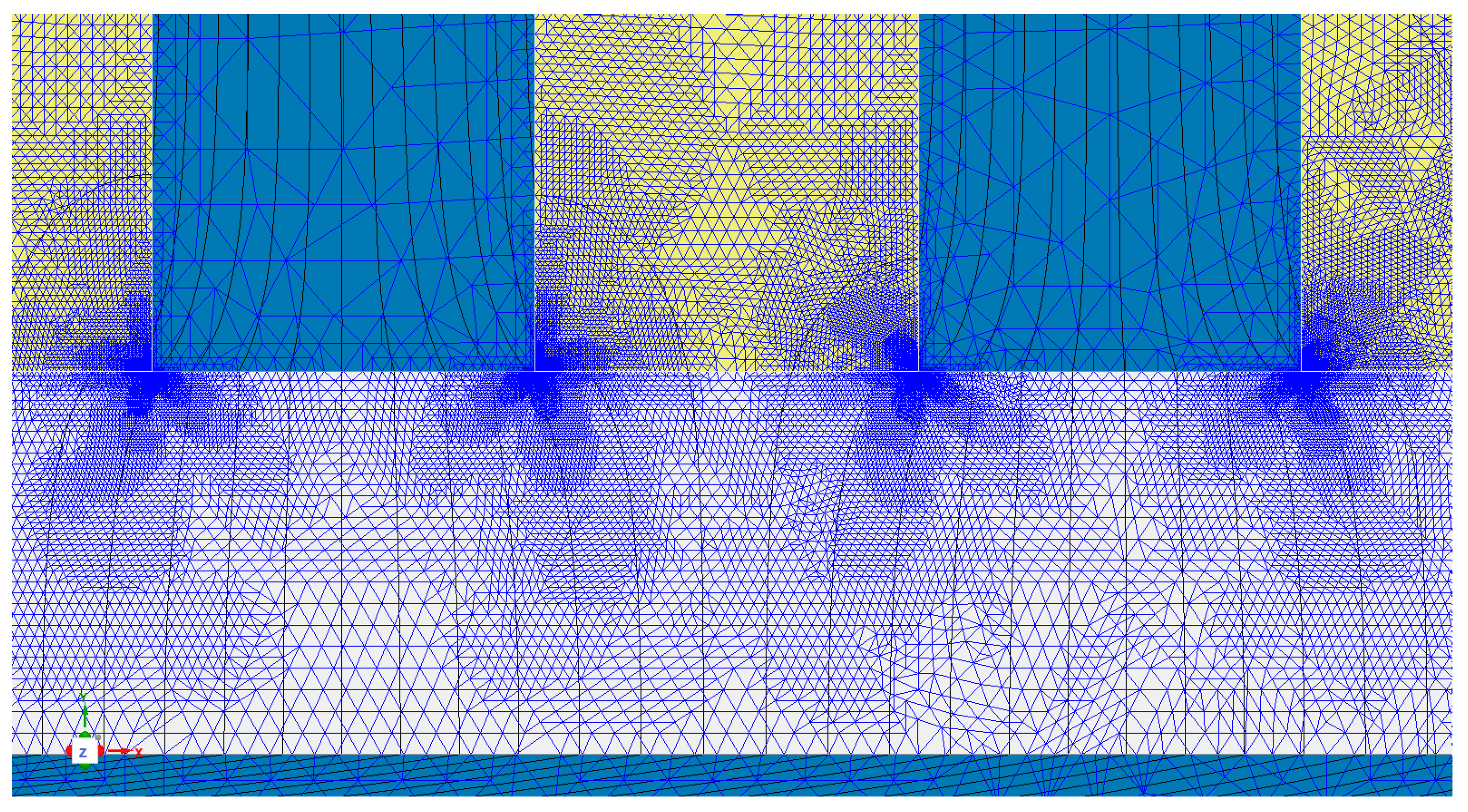
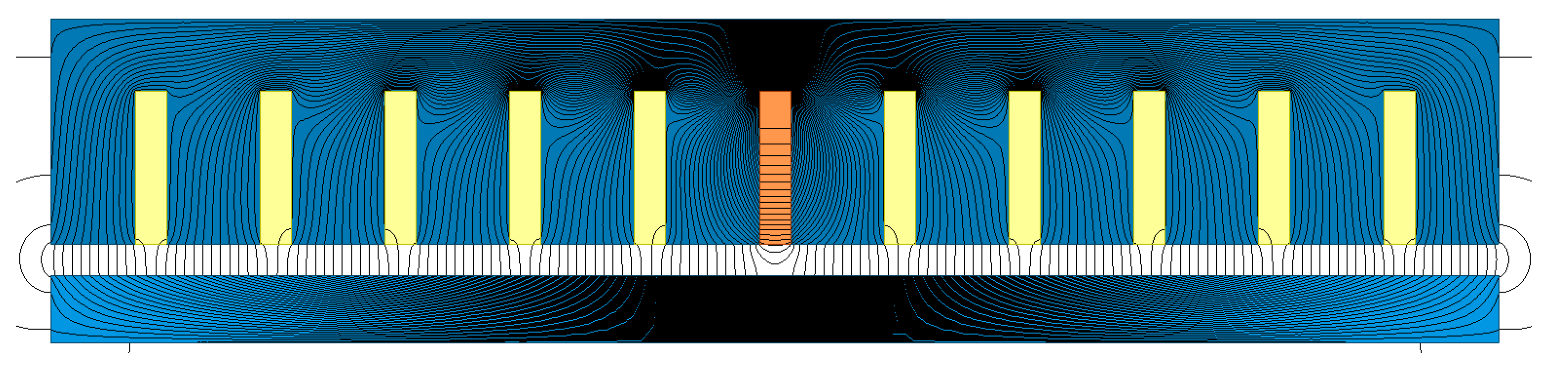
The complete FEM model adopted for a comparison with the analytical calculation of the slotting functions is shown in Figure 5; Figure 6 shows the detail of the mesh around the central slot at the right of the conductor; and Figure 7 shows the analytical and FEM slotting functions curves for different positions of the exploring lines. In the FEM model, the ferromagnetic cores were assumed as ideal (μ_fe = 10⁶ pu).

With the conductor current I_c considered in the FEM model, the ideal normal component B_i of the flux density, occurring in case of a smooth upper core, equals B_i = μ₀·I_c/(2·g); thus, from the actual FEM-calculated distributions B_FEMx(x) and B_FEMy(x), the corresponding FEM slotting functions are β_FEMx(x) = B_FEMx(x)/B_i and β_FEMy(x) = B_FEMy(x)/B_i.

In order to ensure accurate and regular distributions of x and y flux density inside the air gap, the following salient data of FEM simulation were adopted: 27 adaptive mesh refinement iterations; energy error = 4.92·10⁻⁶%; Δenergy = 1.22·10⁻⁵%; CPU simulation time = 508 s; total number of mesh triangles (thousands) = 422; in the conductor = 13.5; in each slot = 10.5; and in the air-gap = 277. The particularly high mesh refinement around the tooth corners is evident, where the field changes quickly in space.

Some remarks can be proposed as the following:

-

by using (35) and (36), the position y inside the air gap along which the slotting function was to be calculated could be defined at any time, while, according to [9] and [12], y had to be predefined at half the air gap width and could not be changed;

-

as can be observed, continuous analytical curves and dashed FEM 2D curves were well superposed for any chosen y position of the exploration line.

7.2. Slotting Functions for “Small” Air Gap Width

Figure 8 shows the single-slot slotting functions β_sy0(x − h·τ_s) with h = −1, 0, 1, for g = 2.5 mm, b_s = 2.5 mm, τ_s = 10 mm. For h = 0, the analytical curve is shown together with the FEM curve [19], with bold lines.

For x/τ_s = ±0.5, β_sy0(±τ_s/2) appears very close to 1. This means that in practice, the single-slot slotting functions of adjacent slots do not interfere by superposition significantly, almost without reciprocal interference; in this situation, the air gap width can be qualified as “small”.

Figure 9 shows the multi-slot slotting function β_y0(x) along the smooth surface (y = 0), for the considered “small” air gap geometry (g = 2.5 mm, b_s = 2.5 mm, τ_s = 10 mm): the red curve was analytically calculated (by (28) and the blue dashed curve, by FEM 2D [19]. Moreover, β_y0(±τ_s/2) is very close to 1, confirming the negligible interference between adjacent single-slot slotting distributions.

Again, for g = 2.5 mm, b_s = 2.5 mm, τ_s = 10 mm, Figure 10 shows the multi-slot slotting function x and y components, as a function of the peripheral position x in the slot pitch τ_s, for different values of the exploring line y position in the air gap: here, the maximum considered harmonic order in (35) was k_M = 21. Also in this case, continuous analytical curves and dashed FEM 2D curves are well superposed, for any y position of the exploration line.

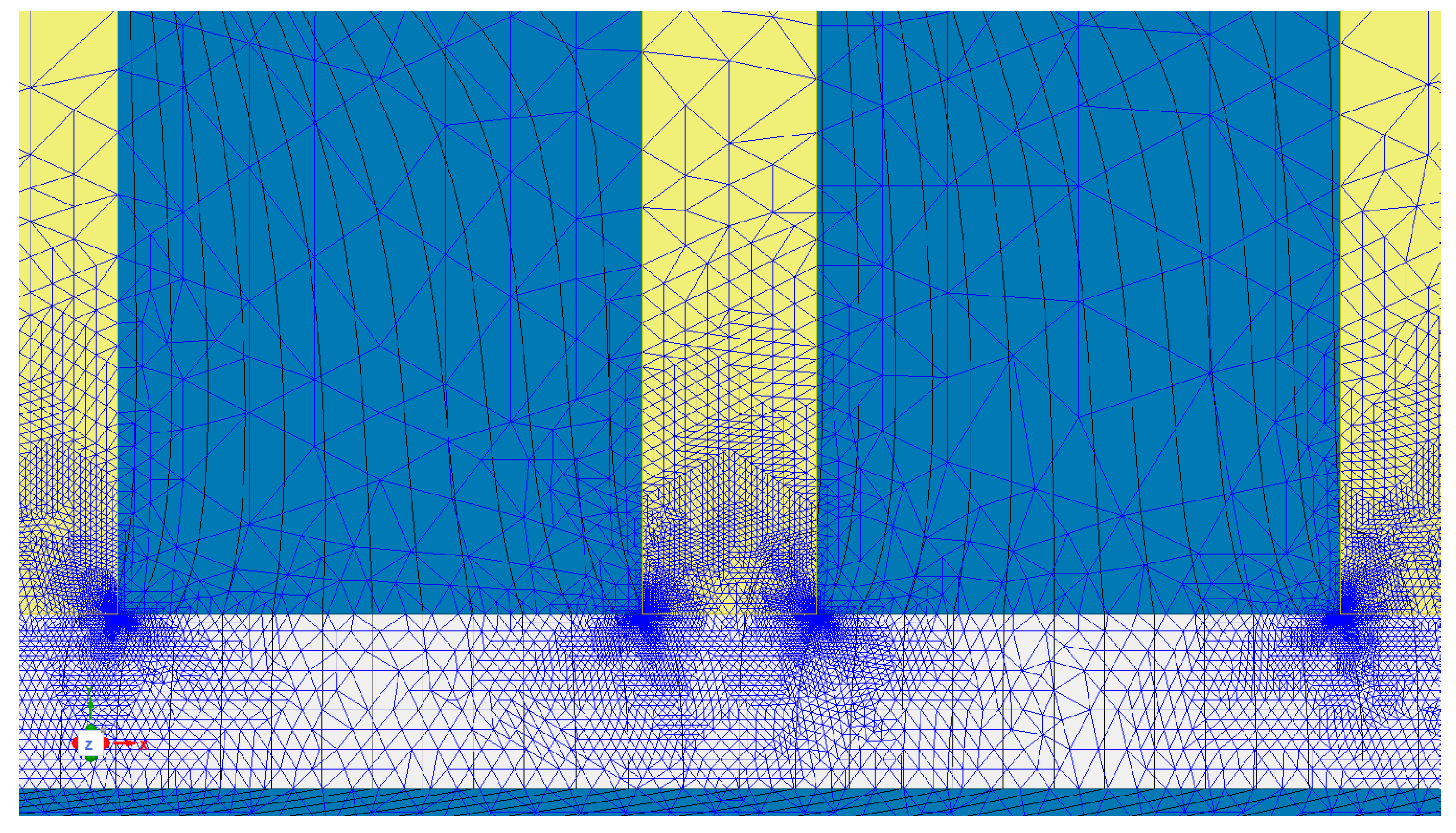
Figure 11 shows the complete FEM model for a “small” air gap (g = 2.5 mm, b_s = 2.5 mm, τ_s = 10 mm:), adopted for a comparison with the analytically calculated slotting functions shown in Figure 10, while Figure 12 shows the detail of the mesh around the central slot at the right of the conductor.

Also for this “small” air gap situation, in order to ensure accurate and regular distributions of x and y flux densities inside the air gap, the following salient data of FEM simulation were adopted: 23 adaptive mesh refinement iterations; energy error = 2.54·10⁻⁵%; Δenergy = 5.76·10⁻⁵%; CPU simulation time = 218 s; total number of mesh triangles (thousands) = 165; in the conductor = 4.6; in each slot = 3.8; and in the air gap = 106.

By observing Figure 12, the particularly high mesh refinement around the tooth corners is evident, where the field changes quickly in space.

However, by comparing these FEM data with the corresponding ones adopted for the “high” air gap simulation, here, the FEM calculation burden was lower than that needed in the case of a “high” air gap.

8. Accuracy of the Slotting Functions with the Choice of the Maximum Harmonic Order k_M

In the following, some accuracy considerations were made about the calculation of the Fourier coefficients, the maximum order k_M of the Fourier series and their consequences on the slotting function distributions.

8.1. Slotting Function Accuracy for “High” Air Gap Width

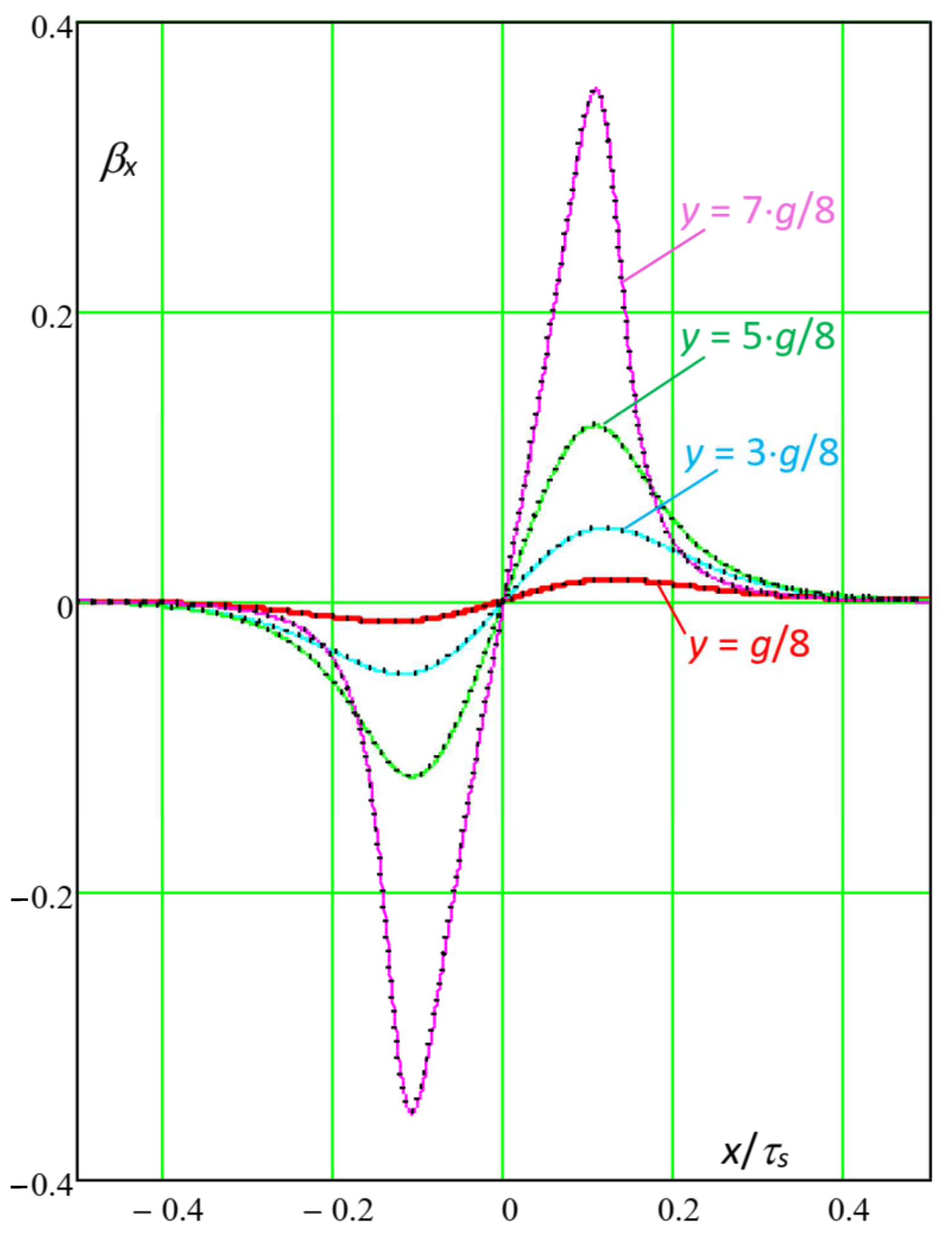
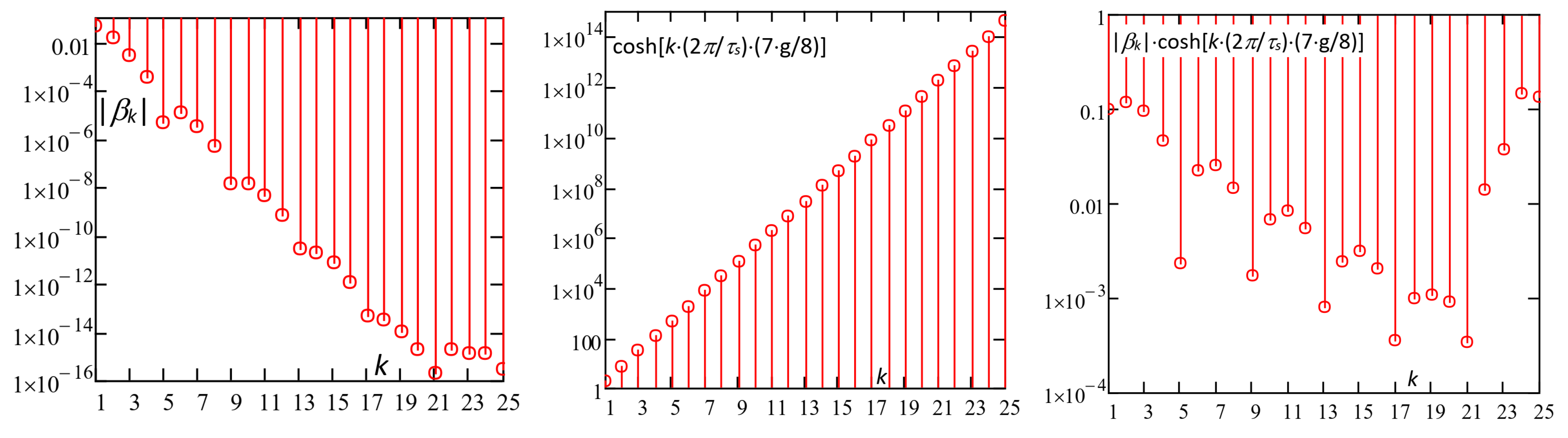
Figure 13 shows a histogram of the |β_k| coefficients of the Fourier series (28), calculated by (33), of the “cosh” factors and of the total factors |β_k|·cosh[k·(2π/τ_s)·(7·g/8)] as a function of harmonic order k, for g = 5 mm, b_s = 5 mm, τ_s = 10 mm (“high” air gap width).

We could make the following remarks:

-

|β_k| decreases with k increasing up to k = 10, while above this order, apparently the amplitude remains almost stationary; however, by observing the |β_k| values for k > 10, it appears that a level around the convergence tolerance TOL = 10⁻¹⁵ was reached and thus, above k > 10 the |β_k| values were inaccurate.

-

As regards the factor cosh[k·(2π/τ_s)·y], for y = 7·g/8 it greatly increases with the increase in the harmonic order k, while the increase is lower for smaller y values.

-

Up to the order k = 10, the total factor|β_k|·cosh[k·(2π/τ_s)·(7·g/8)] decreases, but with a reduction trend much lower than that of |β_k|.

-

For k < 10, the factor |β_k|·cosh[k·(2π/τ_s)·(7·g/8)] shows the typical decreasing behaviour of any Fourier series, while for k > 10, the total harmonic factor tends to suddenly increase; however, this is caused by the numerical error in the estimation of |β_k|, when it falls into the convergence tolerance range.

Figure 14, Figure 15 and Figure 16 show the effect of k_M choice on the slotting function distributions.

The following remarks are valid:

-

for limited values of the y position of the exploring line (y = g/8, 3·g/8, or 5·g/8), the value of k_M has a weak effect on the distribution shape, and the analytically calculated slotting functions appear well superposed with the FEM 2D distributions;

-

if the exploration line inside the air gap is close to the slotted surface (as for y = 7·g/8), the analytically calculated slotting function shape depends on the choice of k_M;

-

if the k_M is too low (k_M = 4, Figure 14), the distribution for y = 7·g/8 is distorted, because the number of harmonics is not enough to reproduce the correct distribution;

-

if the k_M is intermediate (k_M = 7, Figure 15), the distribution for y = 7·g/8 is less distorted, because the number of included harmonics is higher, although not enough to avoid some oscillations;

-

with a k_M = 10 (Figure 7), the distribution for y = 7·g/8 appears well superposed to the FEM distribution and in fact, k_M = 10 is the maximum k_M with a reliable β_kM value (see Figure 9);

-

if the k_M = 11 (Figure 16), the distribution for y = 7·g/8 appears highly distorted, due to the incorrect β_kM value (see Figure 9).

8.2. Slotting Function Accuracy for “Small” Air Gap Width

Here, the accuracy analysis of Figure 13, Figure 14, Figure 15 and Figure 16 was repeated for the considered case of a “small” air gap width.

Figure 17 shows a histogram of the |β_k| coefficients of the Fourier series (28), calculated by (33), of the “cosh” factors and of the total factors |β_k|·cosh[k·(2π/τ_s)·(7·g/8)] as a function of harmonic order k, for g = 2.5 mm, b_s = 2.5 mm, τ_s = 10 mm.

We could make the following remarks:

-

|β_k| decreases with k increases up to k = 21, while above this order, apparently the amplitude increases again or remains almost stationary; however, by observing the |β_k| values for k > 21, it appears that a level around the convergence tolerance TOL = 10⁻¹⁵ was reached and thus, above k > 21 the |β_k| values were inaccurate.

-

As regards the factor cosh[k·(2π/τ_s)·y], for y = 7·g/8, it greatly increases with the increase in the harmonic order k, while the increase is lower for smaller y values.

-

Up to the order k = 21, the total factor|β_k|·cosh[k·(2π/τ_s)·(7·g/8)] generally decreases, but with a reduction trend much lower than that of |β_k|.

-

For k < 21, the factor |β_k|·cosh[k·(2π/τ_s)·(7·g/8)] shows the typical decreasing behaviour of any Fourier series, while for k > 21, the total harmonic factor tends to suddenly increase; however, this is the wrong effect of the inaccurate estimation of |β_k| when it falls into the convergence tolerance range.

Figure 18, Figure 19 and Figure 20 show the effects of k_M choice on the slotting function distributions.

The following remarks are valid, similar to those expressed for Figure 14, Figure 15 and Figure 16:

-

for limited values of the y position of the exploring line (y = g/8, 3·g/8, or 5·g/8), the value of k_M has a weak effect on the distribution shape, and the analytically calculated slotting functions appear well superposed with the FEM 2D distributions;

-

if the exploration line inside the air gap is close to the slotted surface (as for y = 7·g/8), the analytically calculated slotting function shape depends on the choice of k_M;

-

if the k_M is too low (k_M = 7, Figure 18), the distribution for y = 7·g/8 is distorted because the number of harmonics is not enough to reproduce the correct distribution;

-

if the k_M is intermediate (k_M = 15, Figure 19)), the distribution for y = 7·g/8 is less distorted, because the number of harmonics is higher, although not enough to avoid oscillations;

-

with a k_M = 21 (Figure 10), the distribution for y = 7·g/8 appears well superposed to the FEM distribution and in fact, k_M = 21 is the maximum k_M with a reliable β_kM value (see Figure 17);

-

if the k_M = 22 (Figure 20), the distribution for y = 7·g/8 appears highly distorted, due to the incorrect β_kM value (see Figure 17).

Figure 21 shows the histograms of the harmonic amplitudes of the slotting function Fourier series (28), calculated with a multi-slot approach (Equation (30), subscript ms, ×) and with a single-slot approach (Equation (33), subscript ss, □). On the left is a histogram for the case of g = 5 mm, b_s = 5 mm, τ_s = 10 mm (“high” air gap width) and on the right is a histogram for the case of g = 2.5 mm, b_s = 2.5 mm, τ_s = 10 mm (“small” air gap width). All the harmonic amplitudes are referred to as the amplitude of the fundamental components.

We could make the following remarks:

-

In the low harmonic order range (below k_M), the coefficients calculated with the multi-slot approach (Equation (30)) and with the single-slot approach (Equation (33)) had the same values, confirming the correctness of (33).

-

For orders approaching k_M, the two formulas started to give different results, due to the numerical issues about the TOL limit; these issues appeared more critical for the multi-slot approach, because of the superposition of several single-slot distributions in (33), although each distribution had its own inaccuracies.

-

The Fourier coefficients calculated by (33) were accurate up to the k_M order, as shown in the diagrams of Figure 7 and Figure 10.

-

However, above k_M, both the calculation methods ((30) and (33)) gave inaccurate results, as already observed in the histograms of Figure 13 and Figure 17.

9. Conclusions and Perspectives

A method was developed, using the Laplace equation solution in terms of variable separation and Fourier series, for the accurate calculation of multi-slot slotting functions, valid for any geometric air gap parameters, with or without interference among single-slot distributions.

The obtained slotting functions can be used for different y positions of the exploration line in the air gap, and are also quite close to the toothed structure, as needed in the case of surface-mounted permanent magnetic machines.

The calculation of the Fourier series coefficients of the multi-slot configuration were reformulated by transforming the Fourier integrals in terms of a single-slot solution, obtained by conformal transformation.

The accuracy of the slotting functions was studied and the best value for the maximum harmonic order of the Fourier series was obtained by analysing the numerical issues regarding the convergence tolerance limits.

Some slotting function distributions were considered, showing satisfactory correspondence with FEM 2D calculated distributions.

Future studies will concern accuracy improvement in the Fourier series extension and accuracy improvement in the analysis of the magnetic field in the air gap, under no-load and loaded operating conditions, for slotted peripheral configurations.

References

- Chebak, A.; Viarouge, P.; Cros, J. Improved Analytical Model for Predicting the Magnetic Field Distribution in High-Speed Slotless Permanent-Magnet Machines. IEEE Trans. Magn. 2015, 51, 8102904. [Google Scholar] [CrossRef]
- Kim, C.-W.; Koo, M.-M.; Kim, J.-M.; Ahn, J.-H.; Hong, K.; Choi, J.-Y. Core Loss Analysis of Permanent Magnet Synchronous Generator with Slotless Stator. IEEE Trans. Appl. Supercond. 2018, 28, 5204404. [Google Scholar] [CrossRef]
- Di Gerlando, A.; Ricca, C. Analytical Modeling of Magnetic Field Distribution at No Load for Surface Mounted Permanent Magnet Machines. Energies 2023, 16, 3197. [Google Scholar] [CrossRef]
- Di Gerlando, A.; Ricca, C. Analytical Modeling of Magnetic Air-Gap Field Distribution Due to Armature Reaction. Energies 2023, 16, 3301. [Google Scholar] [CrossRef]
- Rahideh, A.; Korakianitis, T. Analytical Magnetic Field Distribution of Slotless Brushless Machines with Inset Permanent Magnets. IEEE Trans. Magn. 2011, 47, 1763–1774. [Google Scholar] [CrossRef]
- Rahideh, A.; Korakianitis, T. Analytical Open-Circuit Magnetic Field Distribution of Slotless Brushless Permanent-Magnet Machines with Rotor Eccentricity. IEEE Trans. Magn. 2011, 47, 4791–4808. [Google Scholar] [CrossRef]
- Zhu, Z.Q.; Howe, D. Instantaneous magnetic field distribution in brushless permanent magnet DC motors. III. Effect of stator slotting. IEEE Trans. Magn. 1993, 29, 143–151. [Google Scholar] [CrossRef]
- Zhu, Z.Q.; Howe, D.; Bolte, E.; Ackermann, B. Instantaneous magnetic field distribution in brushless permanent magnet DC motors. I. Open-circuit field. IEEE Trans. Magn. 1993, 29, 124–135. [Google Scholar] [CrossRef]
- Zarko, D.; Ban, D.; Lipo, T.A. Analytical calculation of magnetic field distribution in the slotted air gap of a surface permanent-magnet motor using complex relative air-gap permeance. IEEE Trans. Magn. 2006, 42, 1828–1837. [Google Scholar] [CrossRef]
- Zarko, D.; Ban, D.; Lipo, T.A. Analytical Solution for Cogging Torque in Surface Permanent-Magnet Motors Using Conformal Mapping. IEEE Trans. Magn. 2008, 44, 52–65. [Google Scholar] [CrossRef]
- Elloumi, N.; Bortolozzi, M.; Tessarolo, A. On the Analytical Determination of the Complex Relative Permeance Function for Slotted Electrical Machines. In Proceedings of the 2020 International Conference on Electrical Machines (ICEM), Gothenburg, Sweden, 23–26 August 2020; pp. 253–258. [Google Scholar] [CrossRef]
- Tessarolo, A.; Olivo, M. A new method for the analytical determination of the complex relative permeance function in linear electric machines with slotted air gap. In Proceedings of the 2016 International Symposium on Power Electronics, Electrical Drives, Automation and Motion (SPEEDAM), Capri, Italy, 22–24 June 2016; pp. 1330–1335. [Google Scholar] [CrossRef]
- Wang, M.; Zhu, J.; Guo, L.; Wu, J.; Shen, Y. Analytical Calculation of Complex Relative Permeance Function and Magnetic Field in Slotted Permanent Magnet Synchronous Machines. IEEE Trans. Magn. 2021, 57, 8104009. [Google Scholar] [CrossRef]
- Wang, M.; Li, H.; Xu, X.; Zhu, J.; Shen, Y. Magnetic Field Analysis of Permanent Magnet Linear Synchronous Motor Based on the Improved Complex Relative Permeance Function. In Proceedings of the 2021 13th International Symposium on Linear Drives for Industry Applications (LDIA), Wuhan, China, 1–3 July 2021; pp. 1–6. [Google Scholar] [CrossRef]
- Lee, S.-H.; Yang, I.-J.; Kim, W.-H.; Jang, I.-S. Electromagnetic Vibration-Prediction Process in Interior Permanent Magnet Synchronous Motors Using an Air Gap Relative Permeance Formula. IEEE Access 2021, 9, 29270–29278. [Google Scholar] [CrossRef]
- Lv, Y.; Cheng, S.; Ji, Z.; Wang, D.; Chen, J. Permeance Distribution Function: A Powerful Tool to Analyze Electromagnetic Forces Induced by PWM Current Harmonics in Multiphase Surface Permanent-Magnet Motors. IEEE Trans. Power Electron. 2020, 35, 7379–7391. [Google Scholar] [CrossRef]
- Carter, F.W. The magnetic field of the dynamo-electric machine. J. Inst. Electr. Eng. 1926, 64, 1115–1138. [Google Scholar] [CrossRef]
- Gibbs, W.J. Conformal Transformation in Electrical Engineering; Chapman & Hall Limited: London, UK, 1958. [Google Scholar]
- Ansys FEM Software: Electronics Desktop, Version 2021R2. Available online: https://ansys.com/company-information/ansys-simulation-software (accessed on 3 September 2023).
Figure 1.
Slot in a multi-slot structure, with infinitely deep slot height, air gap width g and slot pitch τs, slot opening bs (here equal to the slot width); the reference frame, xy, is centred at the point c.
Figure 2.
Single slot with infinitely deep height, air gap width g, slot opening bs (assumed equal to the slot width); here, the adopted reference frame, xbyb, is positioned in corner b.
Figure 3.
Single-slot slotting functions along the smooth surface βsy0(x − h·τs) with h = −2, −1, 0, 1, 2 (continuous lines); central (h = 0) single-slot slotting function βsy0(x) (red bold line = analytical, by (23); blue dotted line = FEM 2D [19]); slotting parameters: g = 5 mm, bs = 5 mm, τs = 10 mm (“high” air gap width).
Figure 4.
Multi-slot slotting function βy0(x) along the smooth surface (y = 0), for g = 5 mm, bs = 5 mm, τs = 10 mm: analytically calculated (red curve, by (27)); FEM 2D (blue dashed curve) [19].
Figure 5.
Multi-slot configuration used for FEM numerical calculation of the slotting functions, with a “high” air gap condition (g = 5 mm, bs = 5 mm, τs = 10 mm): the device consists of 10 slots, with the orange, central one equipped with a current-fed rectangular conductor.
Figure 6.
Detail of the multi-slot configuration of Figure 5, around the central slot at the right of the conductor, with the aspect of the mesh and a few field lines.
Figure 7.
Multi-slot slotting function x and y components as a function of the peripheral position x within the slot pitch τs, for a few values y of the air gap exploring line, for g = 5 mm, bs = 5 mm, τs = 10 mm (“high” air gap width): continuous line = analytical (Equations (35) and (36), max harmonic order kM = 10); dotted lines = FEM [19].
Figure 8.
Single-slot slotting functions along the smooth surface βsy0(x − h·τs) with h = −1, 0, 1, (continuous lines); central (h = 0) single-slot slotting function βsy0(x) (red bold line = analytical, by (24); blue dotted line = FEM 2D [19]); slotting geometric parameters: g = 2.5 mm, bs = 2.5 mm, τs = 10 mm (“small” air gap width).
Figure 9.
Multi-slot slotting function βy0(x) along the smooth surface (y = 0), for g = 2.5 mm, bs = 2.5 mm, τs = 10 mm: analytically calculated (red curve (by (28)); FEM 2D (blue dashed curve) [19].
Figure 10.
Multi-slot slotting function x and y components as a function of the position x in the slot pitch τs, for a few values y of the exploring line, for g = 2.5 mm, bs = 2.5 mm, τs = 10 mm (“small” air-gap): continuous line = analytical (Equations (35) and (36), max harmonic order kM = 21); dotted lines = FEM [19].
Figure 11.
Multi-slot configuration used for FEM numerical calculation of the slotting functions, with a “small” air gap condition (g = 2.5 mm, bs = 2.5 mm, τs = 10 mm): the device consists of 10 slots, with the orange, central one equipped with a current fed rectangular conductor.
Figure 12.
Detail of the multi-slot configuration of Figure 11, around the central slot at the right of the conductor, with the aspect of the mesh and a few field lines.
Figure 13.
Amplitudes of the βk cosine coefficients of the Fourier series (28), calculated by (33), of the “cosh” factors and of the total coefficients |βk|·cosh[k·(2π/τs)·(7·g/8)] as a function of the harmonic order k, for g = 5 mm, bs = 5 mm, τs = 10 mm (“high” air gap width).
Figure 14.
Multi-slot slotting function x and y components as a function of the peripheral position x within the slot pitch τs, for a few values y of the air gap exploring line, for g = 5 mm, bs = 5 mm, τs = 10 mm (“high” air gap width): continuous line = analytical (Equations (35) and (36), maximum harmonic order kM = 4); dotted lines = FEM [19].
Figure 15.
Multi-slot slotting function x and y components as a function of the peripheral position x within the slot pitch τs, for a few values y of the air gap exploring line, for g = 5 mm, bs = 5 mm, τs = 10 mm (“high” air gap width): continuous line = analytical (Equations (35) and (36), maximum harmonic order kM = 7); dotted lines = FEM [19].
Figure 16.
Multi-slot slotting function x and y components as a function of the peripheral position x within the slot pitch τs, for a few values y of the air gap exploring line, for g = 5 mm, bs = 5 mm, τs = 10 mm (“high” air gap width): continuous line = analytical (Equations (35) and (36), maximum harmonic order kM = 11); dotted lines = FEM [19].
Figure 17.
Amplitudes of the βk cosine coefficients of the Fourier series (28), calculated by (33), of the “cosh” factors and of the total coefficients|βk|·cosh[k·(2π/τs)·(7·g/8)] as a function of harmonic order k, for g = 2.5 mm, bs = 2.5 mm, τs = 10 mm (“small” air gap width).
Figure 18.
Multi-slot slotting function x and y components as a function of the peripheral position x within the slot pitch τs, for a few values y of the air gap exploring line, for g = 2.5 mm, bs = 2.5 mm, τs = 10 mm (“small” air gap width): continuous line = analytical (Equations (35) and (36), maximum harmonic order kM = 7); dotted lines = FEM [19].
Figure 19.
Multi-slot slotting function x and y components as a function of the peripheral position x within the slot pitch τs, for a few values y of the air gap exploring line, for g = 2.5 mm, bs = 2.5 mm, τs = 10 mm (“small” air gap width): continuous line = analytical (Equations (35) and (36), maximum harmonic order kM = 15); dotted lines = FEM [19].
Figure 20.
Multi-slot slotting function x and y components as a function of the peripheral position x within the slot pitch τs, for a few values y of the air gap exploring line, for g = 2.5 mm, bs = 2.5 mm, τs = 10 mm (“small” air gap width): continuous line = analytical (Equations (35) and (36), maximum harmonic order kM = 22); dotted lines = FEM [19].
Figure 21.
Histograms of the harmonic amplitudes of the slotting function Fourier series (28), calculated with a multi-slot approach (Equation (30), subscript ms, ×) and with a single-slot approach (Equation (33), subscript ss, □). Left: histogram for the case of g = 5 mm, bs = 5 mm, τs = 10 mm (“high” air gap width); right: histogram for the case of g = 2.5 mm, bs = 2.5 mm, τs = 10 mm (“small” air gap width). All the harmonic amplitudes are referred to as the amplitude of the fundamental components.
Disclaimer/Publisher’s Note: The statements, opinions and data contained in all publications are solely those of the individual author(s) and contributor(s) and not of MDPI and/or the editor(s). MDPI and/or the editor(s) disclaim responsibility for any injury to people or property resulting from any ideas, methods, instructions or products referred to in the content. |
© 2023 by the authors. Licensee MDPI, Basel, Switzerland. This article is an open access article distributed under the terms and conditions of the Creative Commons Attribution (CC BY) license (https://creativecommons.org/licenses/by/4.0/).
Share and Cite
MDPI and ACS Style
Di Gerlando, A.; Ricca, C. Analytical Modelling of the Slot Opening Function. Magnetism 2023, 3, 308-326. https://doi.org/10.3390/magnetism3040024
AMA Style
Di Gerlando A, Ricca C. Analytical Modelling of the Slot Opening Function. Magnetism. 2023; 3(4):308-326. https://doi.org/10.3390/magnetism3040024
Chicago/Turabian StyleDi Gerlando, Antonino, and Claudio Ricca. 2023. "Analytical Modelling of the Slot Opening Function" Magnetism 3, no. 4: 308-326. https://doi.org/10.3390/magnetism3040024