2. The Continuous Crystallizer Case Study
The selected process for the application of the dynamic surrogate modeling approach is continuous crystallization. Crystallization is a non-conventional unit operation aimed at precipitating a solid phase from a liquid solution based on supersaturation conditions of the selected species. Depending on the final product characteristics, the operation can be conducted using batch, semi-batch, or continuous equipment. Although several studies on crystallization can be found in the literature, most of them rarely address the unit from a macroscopic perspective. While batch and semi-batch configurations are conventionally modeled as dynamic units, continuous crystallization is typically analyzed as a steady-state unit. However, because perturbation can affect the operating parameters, the final properties of the product (especially crystal size) can substantially vary over a non-negligible transient.
A simplified scheme of the conventional continuous crystallizer unit is depicted in
Figure 1. As shown, the feed solution is introduced to the unit along with a heating agent (usually steam), providing heat for the partial solvent evaporation. Consequently, the solution concentration exceeds the saturation equilibrium condition, initiating the precipitation of the solid phase. Some relevant aspects of the unit operation layout need to be discussed first in order to accurately define the mathematical model of this unit. Notably, bigger crystals are separated from the finer ones through floatation. Then, the circulating pipe recycles and mixes the finer crystals with the feed. In fact, at the industrial scale, heterogeneous crystallization (i.e., in the presence of pre-existing nuclei) is greatly preferred over homogeneous crystallization due to its much higher nucleation rate, corresponding to a higher productivity. Another significant aspect of the operation relates to mixing; sustained mixing speeds ensure homogeneous conditions throughout the unit volume and enhance the mass transfer rate [
20]. Finally, the barometric condenser is included in the equipment to remove vaporized solvent and dissolved gases from the unit, which typically operates under vacuum to facilitate evaporation. No solid phase is lost from this outlet; solid crystals are instead withdrawn from the product discharge outlet.
Based on the given process description, the dynamic mass balances in the liquid and solid phases for the solute species can be respectively written as follows:
where
is the mass of the solute in the liquid (
l) and solid (
s) phases,
is the crystal mass flowrate for the inlet (
in) and the outlet (
out) solid streams,
is the solute concentration in [kg/m
3] in the liquid streams,
is the volumetric flowrate in [m
3/s], and
is the rate of crystallization per unit volume. Finally,
is the liquid volume inside the crystallization unit, and, assuming that the presence of the solute species does not affect the volume occupied by the solvent, it can be calculated with a mass balance on the liquid solvent phase:
where
is the evaporation rate.
Based on these equations, several observations can be made to define each parameter and reshape the proposed model into a more concise formulation. Firstly, due to the presence of recycling, no outlet liquid stream is necessary, and no inlet crystals need to be considered except for the recirculated fines. Second, owing to the homogeneous conditions within the unit, the properties of the outlet streams match those inside the equipment (e.g.,
). Thirdly, as the outlet solid flowrate, indicative of the process productivity, includes all grown crystals removed from the bottom section of the unit,
can be assumed to be equal to
per hour, except for the fraction α of seeds recycled, which corresponds to 10% of the steady-state mass value. Finally, the density of the liquid phase can be treated as constant, and the evaporation rate is a function of the heating rate (
) expressed by the equation:
where
is the solvent evaporation enthalpy and where the duty is controlled in order to keep the same evaporation rate as nominal steady-state conditions, i.e.,
.
Regarding the interaction between the liquid and solid phases, mass transfer can be neglected due to the sustained mixing rate of the equipment [
21], and the solute precipitation can be modeled as a second-order reaction, according to the example provided by Aghajanian and Koiranen (2020) [
22]. The reaction rate can then be described by the equation:
where
is the reaction kinetic coefficient expressed in [m
3/kg·h].
The final model then becomes
The nominal operating parameters used for this study are listed in
Table 1. When switching to the process dynamic model solution, they are used as the ODE system initial conditions.
The main effectiveness indicator for a crystallization process is the crystal growth ratio, defined as the ratio between the mass of the final crystal product and that of the initial crystal seeds. For this study, it is given by
If the system satisfies the McCabe
law, the linear growth of the crystal can be considered independent of the initial crystal size [
23]. In this case study, as crystals are distributed along the unit based on their mass due to floatation, and the recycled ones are removed from the same crystallizer height, an almost uniform distribution can be assumed. Therefore, the overall linear growth can be calculated as the growth of a single crystal using the equation:
The purpose of this study is to establish a correlation between the indicator and the variation in species concentration in the feed stream by means of a derivative-based surrogate model, which consists of a single differential equation to directly describe the response of crystal growth with respect to the input step disturbance. The choice of a relatively simple phenomenological model helps to evaluate the potential of the metamodeling procedure in terms of computational effort on a single unit before tackling larger and more complex systems. The results, discussed in the corresponding section, demonstrate significant improvements in computational time despite the relatively low complexity of the continuous crystallizer. However, before delving into the results, a comprehensive explanation of the response function-based surrogate modeling approach is provided in the following section.
3. Methodology
This Methodology Section addresses the two main aspects of the surrogate modeling study, namely, the Design of Experiment and the modeling method. In particular, the details regarding the selected sampling strategy and its application to the specific system under analysis are presented in the first subsection, while the fundamentals of the response function-based dynamic surrogate modeling approach are discussed in the second one.
3.1. Design of Experiment
In the DoE step, two main phases can be distinguished, namely, the domain definition and the sample generation. The former aims to select the variation range of the independent variables over which the accuracy of the final model is sufficiently high and no region with considerable deviation from the experimental data can be detected. In some studies, for instance, a repartition of the overall domain into multiple subdomains is performed to improve the accuracy of the surrogate model at the expense of the modeling procedure, which should be repeated as many times as the number of subdomains [
24]. The latter, as mentioned in the introduction, aims to provide a uniform distribution of points to ensure homogeneous representation of all parts of the domain.
For this study, the feed properties, i.e., flowrate (Qin) and concentration (Cin), were selected as independent variables. Specifically, to model the continuous crystallization dynamics, a perturbation domain within the ±50% range with respect to the nominal operating conditions was considered over a 10-h simulation. This choice allowed us to cover a 100% operating window and have a sufficiently heterogeneous profile without falling into singular cases. Thus, this approach was used to obtain both the DoE and the validation set profiles. The importance of the difference between the validation set and the DoE is based on the fact that, since the model is built to be as compliant as possible with respect to the DoE points, it will likely comply with similar trends, but only a robust model will minimize error even for very different values of the independent variables.
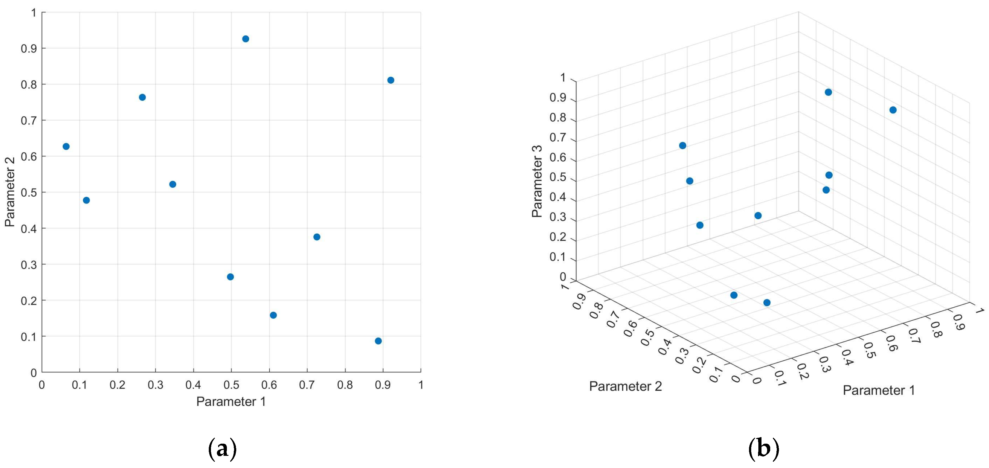
Regarding point generation, the sampling strategy selected for this research was Latin Hypercube Sampling (LHS) [
25]. This near-random sample generation methodology is particularly suitable for once-through surrogate modeling since it provides uniform domain filling and ensures that two points are never aligned in the orthogonal direction with respect to the axes of independent parameters. For a better understanding, examples of LHS for bidimensional and tridimensional domains are shown in
Figure 2 (a and b, respectively); it can be seen that, given the number of points
n, the space is partitioned into an
n × n chessboard, and data points are distributed on random locations within squares that do not belong to the same row or column of any other point.
The presented research employs LHS in two cases. The first one concerns the generation of 10
Qin ×
Cin ×
t combinations for the system step perturbations, 5 for the DoE profile and 5 for the validation set. Then, LHS will be used to generate data samples for modeling from the growth vs. time trend whose size will range from 10 to 100 points. The independent variable profiles are thus obtained, and the outcomes of the related model simulation are reported in
Section 4.1. From an operational point of view, the LHS was performed using the dedicated function
lhsdesign, available in Matlab
®, so that the same software was used for the sampling and the modeling phases. Details concerning the latter are provided in the next section.
3.2. Response Function-Based Dynamic Surrogate Modeling
The surrogate modeling methodology proposed in this research is inspired by the derivative-based surrogate modeling approach proposed by Di Pretoro et al. (2022) [
14] for an ethylene oxide process study and readapted to the continuous crystallization unit. The objective of this work is to use a single differential equation to correlate crystal growth and inlet parameters, expressed as deviation variables with respect to the nominal operating conditions. The model approach can be assumed to be analogous to that of the Response Surface Methodology [
5]. However, in this case, the response surface is not modeled as an explicit function but as a differential response function, according to the well-established characteristic equations [
26]. Although the system to be modeled is complex or could be composed of several sub-systems, in a series or parallel coupling layout, sometimes the correlation between the system outlet and the input variables can be simplified by low-order differential equations, without the need of a multiple sub-model combination. Examples of the parametrical differential form of a first- and second-order response function are reported in Equations (11) and (12), respectively:
The known terms used in these equations refer to the characteristic parameters of the process dynamics (
τ,
ω,
ξ, etc.) and to the coefficients related to the specific system that is modeled (
A,
B,
D,
E, etc.), while
u and
y represent the independent and dependent variables, respectively. To select the most suitable characteristic differential equation, the approach can be either knowledge-based or automated. The former requires the analysis of the phenomenological model trend and its association with an already known low-order model by the decision maker, while the latter consists of iterative automated tests with equations of different orders and the selection of the equation corresponding to the highest compliance. In the first case, once the most compliant function has been detected, the function coefficients are obtained by solving the Mean Absolute Error (MAE) minimization problem using an optimization algorithm in the form of
where
is the value of the dependent variable corresponding to the DoE sampling, while
is the respective value obtained by the dynamic surrogate model. In the second case, this procedure is replicated for the entire set of differential response functions.
For this study, the most suitable model was detected by the authors, and, as already mentioned, the error minimization was performed by using Matlab
® built-in optimization functions. The same software was also used for profile graphics and data post-treatment. With regards to the latter, the performance indicators used to assess the accuracy and computational efficiency of the surrogate model are the machine computational time and the Normalized Mean Square Error (NMSE) over the 10-h simulation, respectively. The NMSE can be defined as
where
is the average value of one experimental point in the case of multiple sets. In the case of an automated procedure, this indicator could be used for the a posteriori selection of the most suitable differential response function among those that have been tested.
The results concerning the sampling and the modeling step are presented and discussed in detail in the following section.
4. Results and Discussion
This section includes both the DoE and the modeling phase results. In the first subsection, the deviations of the independent parameters and the related response profiles are presented for both the DoE and the validation set. In the second subsection, the comparison between the surrogate model and the crystallizer growth indicator profile is discussed, and performance indicators for the proposed modeling methodology are calculated.
4.1. Dynamic Trend Profiles
As a first step, the external perturbation profiles were generated according to the LHS method to obtain the DoE dataset and the validation profile to be compared to the modeling phase outcome, as reported in
Figure 3 and
Figure 4, respectively.
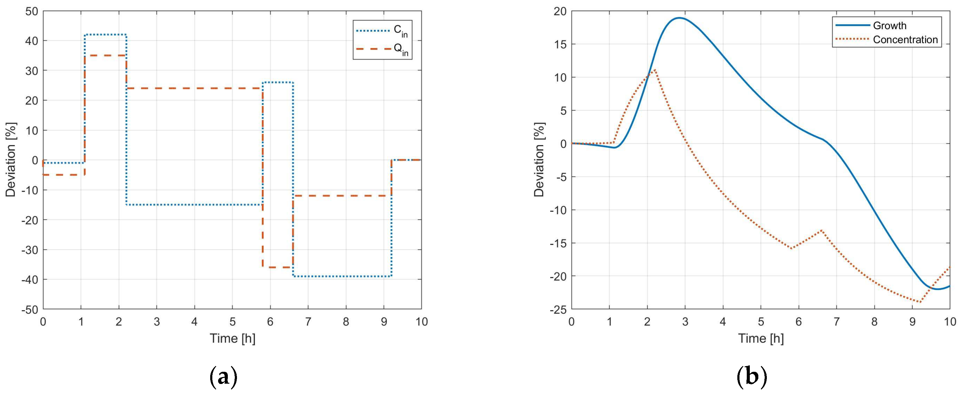
The step deviations for inlet flowrate (red dashed line) and concentration (blue dotted line) correspond to a linear growth deviation (blue line) with respect to the steady-state value under nominal operating conditions. Thus, based on the trend in
Figure 3b, data samples ranging in size from 5 to 100 were generated to perform a sensitivity analysis of the modeling procedure accuracy.
However, the obtained results not only serve the purpose of providing points for the sample generation and the final model validation but, in this case, they are also exploited to decide which response function order can best model the continuous crystallizer unit. As can be observed in
Figure 3b, the solute concentration in the unit exhibits a first-order dynamic behavior, consistent with the model related to Equation (6). Conversely, the dynamic trend of crystal linear growth is much more difficult to deduce using the model equations since it does not directly appear in any of them; it is the result of further operations based on the phenomenological model solution. A second-order response function was then tested as a possible surrogate model for the linear growth dynamics correlation with respect to the process input parameters. The resulting outcome is reported and analyzed in the following section.
4.2. Dynamic Surrogate Model
The modeling phase, based on the methodology previously proposed by the authors [
14], was performed first. Before analyzing the results, it is worth noting that all variables presented in this section are expressed as deviation variables with respect to the nominal steady state, defined as
Therefore, the initial conditions are always set to [0,0], and all dependent variables are expressed as a percentage of the steady-state ones.
Figure 5 shows the results for a first attempt at crystallization modeling based on a global second-order response over the entire domain. In particular, the graph refers to the result options that best fit the first step response, when accounting for the concentration perturbation only. As can be seen, despite the similar trend in terms of positive/negative slope and proportional gain, the error with respect to the other perturbations increases along with the simulation’s elapsed time. Several attempts to improve the quality of the overall profile have been carried out both for coupled and standalone disturbances, but whenever a more compliant dynamic trend is obtained over a given region, the mismatch increases for other scheduling windows. This inconvenience is due to the fact that the characteristic parameters of the model, such as the characteristic frequency
and damping factor
, are not constant during the operation because of the variation in the system characteristics. In particular, the variation in volume during the operation, due to the inlet flowrate perturbation, affects the unit residence time and the system inertia. It is important to note that, in the previous study where this methodology worked for the entire window scheduling [
14], the model correlation was carried out for the product flowrate as a function of the reactant one, and the system in between was a closed-loop system with fixed design and operational parameters.
Therefore, to deal with this issue, a domain partition was performed and the modeling procedure was repeated with a subdomain-wise approach, as suggested in the literature [
27]. The obtained results are reported in the following section along with the analysis of the model performance indicators.
4.3. The Domain Partition-Based Modeling Approach
In the light of the previous results, the first step of the corrected procedure was to partition the domain according to the discretization of step disturbances. Apart from this modification, the following modeling phase was carried out exactly as described in the Methodology Section for each subdomain independently, regardless of the time interval size.
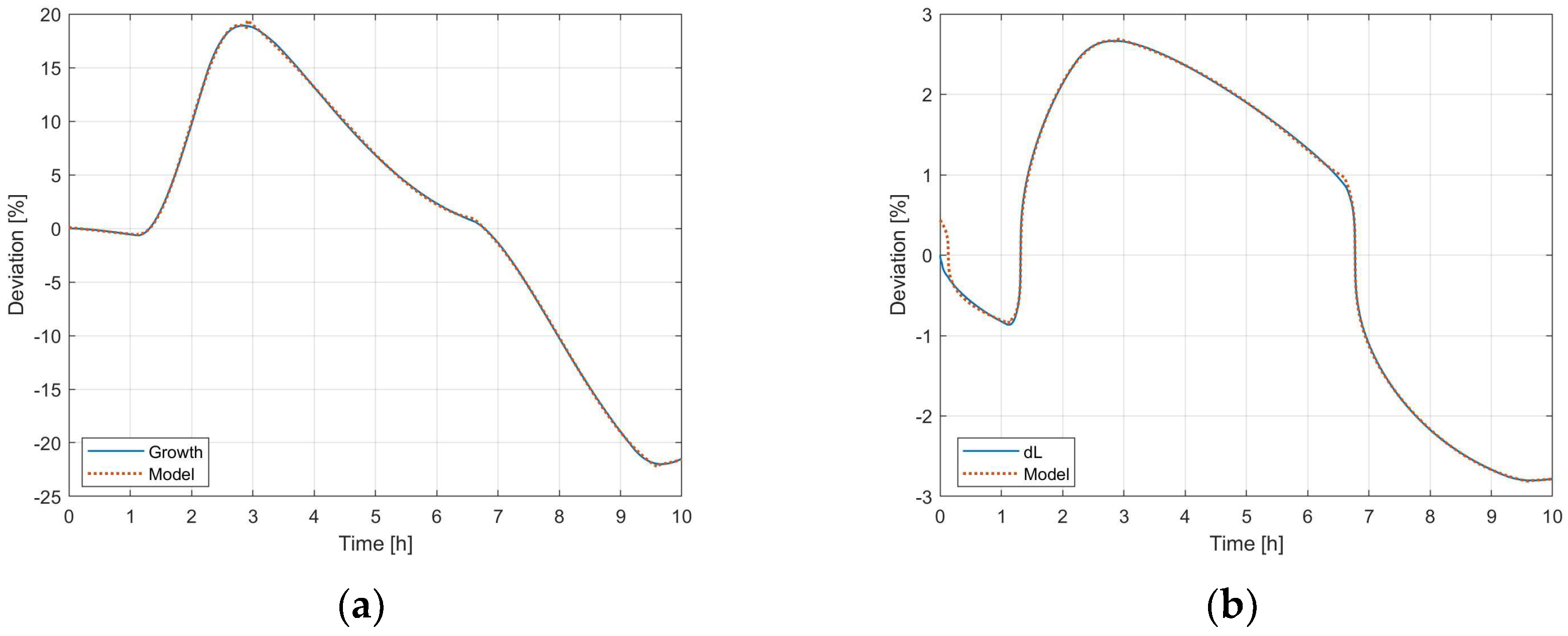
Therefore,
Figure 6 shows the results for the domain-wise second-order differential equation model with a 2000-point sample. In this case, the global model is characterized by as many [
] binaries as its subdomains, i.e., 6. Compared to the previous approach, the new model proves to be very accurate (NMSE equal to 99.9358% and 99.9931% for mass and linear growth, respectively) and meets the initial expectations in terms of compliance with the DoE trend. Predictably, the main criticalities can be observed at the subdomain boundaries where the error is slightly higher, and non-differentiable singular points can be noticed, though without causing any relevant issue to the overall trend. Furthermore, when applying the cubic root to shift from mass to linear growth, the errors are further mitigated, except for points close to the initial condition.
Regarding computational performance, the calculations were performed using a laptop running Matlab
® version 2023b on the Windows 11 operating system, equipped with a 13th-Gen. i9 2.60 GHz processor and 64 GB of RAM. The resulting trends of computational time and model accuracy as a function of the sample size are reported in
Figure 7a and
Figure 7b, respectively.
The value of the Normalized Mean Square Error, calculated as explained in Equation (14), is reported in
Figure 7a for both the phenomenological and surrogate models. Generally, the NMSE trend increases with the increasing number of points, as expected due to the accuracy improvement. However, it can be observed that compliance with the benchmark results is achieved much faster by the rigorous model, with an almost negligible mismatch for samples with more than 125 points. Conversely, the surrogate model follows a hyperbolic trend with higher eccentricity, and the error increases faster when approaching small samples. Nevertheless, the overall mismatch with respect to the phenomenological model becomes lower than 5% for 250 points and falls below 1.5% for samples with more than 500 points.
Computational time exhibits a linear trend for both the phenomenological and surrogate models as the number of points to be calculated increases. However, a remarkable difference can be clearly noticed when comparing the two: the solution of the entire model with respect to a single second-order differential equation requires a computational time that is more than two orders of magnitude higher, despite the low complexity of the crystallizer unit. Based on these results and considering the low slope of the computational time behavior with respect to the sample size, it can be concluded that a sample size of 500 points is a good compromise between model accuracy and computational effort; if a higher accuracy is required and a small increase in model solution time can be tolerated, the 1000-point sample is definitely the best option, corresponding to a totally feasible computational performance.
Finally, the same procedure was repeated on the validation dataset using the optimal number of 1000 points per subdomain sample. The results are presented in
Figure 8. From a qualitative point of view, the same remark as for the DoE-based trends remains valid. In particular, the NMSE for the mass and linear growth functions is equal to 99.9682% and 99.9964%, respectively. Cuspid points can still be detected in correspondence with step perturbation changes, but even in this case they do not considerably affect the overall accuracy except in proximity of the linear growth trend initial conditions. Therefore, based on the obtained outcome, the surrogate modeling approach exploiting domain partition for the description of continuous crystallizer dynamics can be validated.
5. Conclusions
In the presented research, a surrogate model was developed to describe the dynamics of a continuous crystallizer unit by tackling some critical issues that were encountered. The analysis of these criticalities led to important methodological considerations, which can be summarized as follows:
When the system properties undergo significant variations during operation scheduling, a single model cannot fully describe the process behavior throughout the entire simulation window. In this case, multiple modeling phases over a domain partition should be conducted;
Conversely, for the simulation of a single transient, employing a response function-based dynamic surrogate model yielded highly accurate results in terms of independent variable trends and in the analysis of the indirect outcome parameters;
Additionally, for a single modeling region, the sample size corresponding to the best compromise between computational effort and accuracy can be identified;
The use of surrogate models for dynamic simulation substantially enhances computational efficiency while maintaining a high level of accuracy. However, full automation is currently unattainable, as a preliminary analysis of the system physical behavior is necessary to select the most suitable modeling methodology.
Therefore, considering the significant outcomes discussed above, further testing and development of the presented procedure are worthwhile. The direct correlation between the input and output variables of interest through a single differential equation, capable of replacing the entire model with good accuracy, exhibits considerable potential in terms of computational time reduction. Therefore, this approach could enable applications such as Real-Time Dynamic Optimization and model predictive control to be used for a broader range of process systems, which currently demand extensive calculation times. Nevertheless, the proposed procedure requires substantial improvements before scaling up to more complex systems. The unconditional use of domain partition might indeed present a notable drawback in terms of computational performance for process systems with highly irregular behavior or wide operating windows. In such cases, the number of required partitions may significantly increase, necessitating adjustments to characteristic parameters for each iteration. Moreover, when dealing with more complex systems, the correlation between input and output variables overlooks the local feasibility limitations of individual units, potentially yielding operating profiles that cannot be attained in practice.
In conclusion, building upon the initial step carried out in this study, further research will focus on developing a comprehensive framework for applying the response function-based dynamic surrogate modeling methodology to process systems. This endeavor will address the aforementioned challenges and explore potential solutions to feasibility issues through a rigorous approach.


