
Cooperative Robot Manipulators Dynamical Modeling and Control: An Overview


Department of Mechanical and Aerospace Engineering, University of California Davis, Davis, CA 95616, USA
Dynamics 2023, 3(4), 820-854; https://doi.org/10.3390/dynamics3040045
Submission received: 1 November 2023
/
Revised: 3 December 2023
/
Accepted: 6 December 2023
/
Published: 11 December 2023
Abstract
:Robot manipulators possess the capability to autonomously execute complex sequences of actions. Their proficiency in handling challenging and hazardous tasks has led to their widespread adoption across diverse sectors, including industry, business, household appliances, rehabilitation, and many more. However, certain tasks prove to be challenging for individual robots, primarily due to constraints in their structure and limited degrees of freedom. Cooperative robot manipulators (CRMs) emerge as a compelling solution when dealing with large, heavy, or flexible payloads. The utilization of CRMs offers a host of benefits, including enhanced manipulation performance achieved through the synergy of sensing and actuation capabilities or by tapping into increased redundancy. Numerous techniques have been devised for the control and dynamical modeling of CRMs. Nevertheless, the field continues to present technical challenges and scientific inquiries. To inspire and facilitate further research and development in this realm, this review aims to consolidate the current body of knowledge pertaining to CRMs kinematics, dynamics modeling, and various control methodologies used for payload manipulation via CRMs.
1. Introduction
With recent advances in robotic technology, the adoption of multiple robots performing a task cooperatively, such as moving a payload, in lieu of a single robot, has gained broad research interest. Here, the term cooperative means the collaboration of multiple robots executing a task simultaneously. The limits in the structure of a robot prevent a sole robot from operating on large, unbalanced, or flexible payloads. On the other hand, cooperative robots show better performance in tasks such as grasping, gripping, lifting, transferring, lowering, and approaching an object. Hence, the driving force behind the creation of a cooperative robotic system stems from its superior capabilities compared with a single robot. This advancement aims to enhance the functional abilities of human operators, enabling the successful completion of challenging tasks, including managing hefty loads (e.g., see references [1,2,3]), intricate assembly procedures [4], efficient pick-and-place operations [5,6], and more.
Drawing from the existing literature, the significant challenges within the domain of cooperative robot manipulators (CRMs) encompass two primary problems: (1) the intricate task of modeling the dynamical system and (2) the formulation of an effective control scheme. Cooperative robot systems lend themselves to diverse approaches for kinematic and dynamic modeling, presenting a spectrum of techniques to choose from. Similarly, a variety of control methodologies, such as linear control theory, nonlinear control, and intelligent control, among others, are applicable. Each modeling approach possesses its own set of advantages and limitations, which in turn can propose distinct control strategies. Given the relative novelty of cooperative robot control as a research area, the predominant focus has been on introducing and contrasting different control methods. An illustrative depiction of this concept is shown in Figure 1, where multiple robots collaborate to manipulate a load within their workspace. Within this context, the payload may be affixed to each robot via either a fixture or an end-effector, and the robots have rigid links and joints that are either revolute or prismatic. The “workspace” denotes the spatial region within which the payload can maneuver. The subsequent sections provide a more precise definition of cooperative robot manipulators. Furthermore, these sections elucidate the rationale behind the need for a comprehensive survey paper dedicated to this specific subject.
1.1. Background
The system of CRM consists of multiple manipulators that form a coupled robotic system with a closed-chain mechanism, as shown in Figure 1. CRMs do not have a specific agreed-upon definition. Dual arm manipulation, human–robot cooperation (a complete literature review of human–robot interaction is presented in [10]), mobile and fixed-based cooperative manipulators, cooperation of unmanned aerial vehicles, space multiarm robotics, and many other forms of cooperation can be categorized under the definition of CRMs. Any form of multiple dynamical system (e.g., robot manipulator, human, …) interactions can be recognized as CRMs.
The collaborative manipulation of solid objects represents a formidable challenge and an actively explored research field. This paper primarily focuses on fixed-based cooperative robot manipulators, i.e., CRMs, which are employed for the handling of rigid objects. By leveraging multiple robots working in concert to execute tasks, new horizons have opened up for the utilization of robot arms and their applications. CRMs hold the potential to be tailored for a wide spectrum of applications, as outlined in Table 1. In general, the deployment of multiple robot manipulators offers opportunities to enhance productivity, reduce labor costs, and enhance safety across various industries. The synchronized movement and manipulation of multiple robot arms can be optimized to achieve the highest levels of efficiency and precision. The utilization of CRMs offers a multitude of advantages, including the following:
- Increased Productivity: Cooperation allows for parallel execution of tasks, resulting in higher productivity compared with a single robot. CRMs can work simultaneously on different parts of a task, reducing overall completion time.
- Enhanced Task Complexity: Complex tasks that may be challenging or impossible for a single robot arm can be tackled by CRMs. Each arm can specialize in a specific aspect of the task, enabling the completion of intricate operations.
- Flexibility and Adaptability: CRMs offer flexibility in adapting to different tasks and environments. The modular nature of the system allows for easy reconfiguration and allocation of robot arms to specific tasks based on requirements.
- Fault Tolerance and Redundancy: In case of a failure or breakdown of one robot’s joint, the other joints can continue to work, ensuring that the overall task progresses. Redundancy in the system improves fault tolerance and system reliability.
Regardless of the aforementioned benefits, employing CRMs comes at the cost of complexity for mathematical modeling, control, and coordination. CRMs are kinematically and dynamically coupled and usually overactuated systems. Overall, the following disadvantages have been detected in the literature:
- Increased Complexity: Coordinating the movements and actions of multiple robot arms requires sophisticated algorithms and communication protocols. The complexity of system design, synchronization, and control can be challenging and may require advanced programming and planning.
- Communication and Coordination Overhead: Effective cooperation among multiple robot arms necessitates robust communication and coordination. The need for exchanging information, synchronizing actions, and avoiding collisions can introduce communication overhead and latency.
- Cost and Maintenance: Implementing and maintaining a multirobot arm system can be costly. Each additional robot arm adds to the hardware and maintenance expenses, requiring regular calibration.
- System Scalability: Scaling up a multirobot arm system to accommodate a larger number of arms may introduce additional challenges. Ensuring seamless coordination and efficient task allocation becomes more complex as the number of robot arms increases.
- Limited Workspace: When multiple robot arms operate in a shared workspace, they need to be carefully coordinated to avoid collisions and ensure safe operations. The available workspace may restrict the number of robot arms that can operate simultaneously.
It is important to note that many of these disadvantages can be mitigated or overcome with careful system design, appropriate algorithms, and advances in technology. As research and development in multirobot arm systems continue, the advantages are expected to outweigh the disadvantages, making them increasingly viable and beneficial in various applications.
1.2. Motivation
Advancements in the realm of cooperative robots hinge upon the evolution of robotic structures, the facilitation of collaboration devoid of human intervention, and the deployment of intricate control algorithms. Driven by the absence of comprehensive surveys and the distinct demands of this domain, this article aims to assess and underscore the distinct prerequisites essential for the evolution of CRMs. Drawing upon significant research endeavors conducted thus far, the focus primarily centers on dynamical modeling and the execution of control methodologies. These aspects are necessary and challenging for achieving efficient models and fully autonomous CRMs. The ultimate goal is to make them not only functional but also reliable for a wide range of applications in the near future.
Acknowledging the abundance of published papers on the topic of robot collaboration, particular attention has been directed toward peer-reviewed works that explore fixed-based cooperative robot manipulators engaged in object handling. In particular, this survey studies the following subjects: (1) an overarching exploration of the dynamics and kinematics modeling of both robots and payload, encompassing challenges and advancements; (2) a concise compilation of diverse control algorithms employed for payload manipulation and regulation, accompanied by identified limitations, technical challenges, and prospective pathways for future research.
It is worth clarifying two points: (1) In this paper, collaborative robots are exclusively considered, excluding parallel mechanisms. A parallel mechanism is a type of mechanical arrangement in which multiple rigid links are connected to a fixed base and a moving platform through multiple joints. On the other hand, cooperative robots are defined as multiple agents which are interacting with each other for task execution. The key distinction is the ability of CRMs to interact safely and effectively. Readers are referred to [44,45,46] for more information regarding parallel mechanisms. (2) In this survey, the primary emphasis is placed on fixed-base robotic arms; however, depending on the context, mobile-based robots may also be examined. The key distinction is that fixed-base robotic arms are stationary and rely only on joint motion and coordination to manipulate the object within the reach of their fixed bases, while mobile-based robotic arms, e.g., humanoid robot cooperation [30], have the added advantage of mobility, allowing them to adapt to different scenarios and locations. This mobility provides greater flexibility in navigating around obstacles or accessing different locations within the environment. A discussion of mobile cooperative robots can be found in [47,48]. Evidently, addressing the modeling and control aspects of cooperative robots with fixed bases presents a heightened level of complexity, necessitating the utilization of advanced techniques and tools to tackle the problem effectively.
1.3. Contributions and Organization
By providing an all-encompassing examination of noteworthy achievements and unresolved challenges within the domain of cooperative robot manipulators, this work can serve as a valuable resource for the robotic research community. This survey has the potential to diminish redundancy in research efforts, facilitate the pinpointing of critical bottlenecks in this domain, and greatly enhance the capacities of forthcoming CRM systems. As far as the authors are aware, no prior endeavor has been undertaken to assemble such an exhaustive survey within this particular realm. The remainder of this paper is organized as follows: In Section 2, an extensive examination of the dynamics and kinematics of CRM systems is presented. Section 3 offers a thorough survey of diverse control methodologies employed for regulating robots, payloads, and achieving specific problem objectives. Lastly, Section 4 encompasses the conclusion and prospects for future endeavors.
2. Dynamics and Kinematics Modeling
A precise CRM model, ensuring accurate control design and facilitating simulation studies, is indispensable for developing control methodologies. This necessitates preliminary exploration of a well-defined mathematical model along with rational system parameters. Typically, a standard model encompasses both the dynamics and kinematics aspects of robots and the payload. Considered here is a system of N robots, each equipped with joints, securely grasping and moving a payload as illustrated in Figure 2.
In this section, exploration unfolds into the domain of dynamical modeling and its associated challenges. To provide a structured overview, commencing with the presentation of the robots’ dynamics in Section 2.1, the dynamics of the payload are subsequently explored in Section 2.2. Following this, attention turns to two key aspects: the closed-chain constraint and degree of freedom, addressed in Section 2.3, and the load distribution among robots, detailed in Section 2.4. To conclude, two significant issues are tackled: the augmented model for robots and payload interactions in Section 2.5 and the formulation of grasping strategies in Section 2.6. Additionally, less explored topics in this domain are introduced in Section 2.7.
2.1. Robot Modeling
The dynamics of a robot manipulator can be presented in either joint space or task space, depending on the context and the goals of the analysis or control. Joint-space modeling focuses on describing the robot’s motion and behavior in terms of its joint angles and/or positions. Task-space modeling describes the robot’s motion and behavior in terms of its end-effector’s spatial position and orientation. In the context of CRMs, task-space modeling may happen at the end-effector, , or the payload frame, . The merits and drawbacks of adopting either modeling approach are listed in Table 2.
The dynamics of the ith robot in joint space can be modeled as
where is the vector of joint coordinates, is the inertia matrix, is the matrix accounting for centripetal and Coriolis effects, is the gravity vector, is the Jacobian matrix (usually assumed to be nonsingular, i.e., full-row rank), is the vector of forces and moments (henceforth called wrenches) applied by the object at the end-effector, and is the vector of wrenches applied at the joints. Caution should be exercised when determining the sign of wrenches. In other words, the wrenches exerted by the robot on the payload are equal in magnitude but opposite in direction to the wrenches applied by the payload on the robot’s end-effector, i.e., , where is the wrench vector applied by the object to the robot [49]. Hence, all equations in the dynamics of CRMs should be written accordingly. It is crucial to recognize the interconnection between the robots through the wrench parameter. The wrench value depends on the motion of the payload, which, in turn, is influenced by the movements of all robots. Consequently, there is a form of information exchange between the robots through the wrench. The following properties of the robot are required for the subsequent development [50]:
Property 1.
The inertia matrix is a uniformly bounded positive definite symmetric matrix for all .
Property 2.
The matrix is skew-symmetric, so for all
Property 3.
The dynamic model in Equation (1) is linear in a set of basic dynamic parameters and can be written as
where is the so-called dynamic regressor matrix, and is the vector of dynamic parameters.
Property 1, comes from the physical fact that the inertia matrix, , is inherently positive definite (PD). The proof for skew-symmetry property can be found in [50]. By combining the dynamics of all N robots, the comprehensive dynamics of CRM can be written as [51,52,53]:
where , and , .
It is possible to present Equation (1) in task space, as demonstrated in many papers, such as [54,55]. In the literature, the primary motivation for this transformation is to combine the dynamics of the robots and the payload, as elaborated in Section 2.5. To obtain the dynamics of the ith manipulator in task space, the following relations between the velocity and acceleration of the joints and end-effector are employed:
where and are the velocity and acceleration of the end-effector, respectively. Using the above equalities with some modifications, the task-space equation can be presented as
where:
The dynamical model presented in this section can be adapted according to the particular problem at hand. This may involve introducing modifications such as incorporating disturbance terms, accounting for joint mechanism (JM) dynamics, employing a task-space model, and more. In the following sections, some of the dynamical model adaptations documented in the literature are examined.
Modification of Robot Dynamical Model
The dynamical model as described in Equation (1) is subject to modification in accordance with the specific requirements of the problem at hand. Several alternative approaches for representing this dynamical model are as follows:
Actuator dynamics: It is possible to combine the robot and actuators’ dynamics as presented in [51,56,57]. In this way, a model can be obtained which can be utilized for low-level control. The interface torque between the JM and the jth robot link can be described by
where , , and are the JM moment of inertia, the gear ratio, and friction coefficient, respectively. The superscript indicates the value of the jth joint of the ith robot. By combining the above equation and robot dynamics, the system can be presented as a function of the torques that have been produced in the actuators. For instance, if the actuators are DC motors, then is the induced torque of the motor, where is the current in the motor and is the motor constant. From this equation, the voltage of the DC motor can be presented in the dynamical model [51].
2.2. Payload Modeling
The dynamics and kinematics of manipulators are coupled because the contact wrenches in all robots interact through the payload. The dynamic coupling effects can be measured using the dynamics of the payload. Hence, modeling the payload is a crucial stage. In terms of identifying the payload, we can distinguish three groups of research:
- Studies that presume full knowledge of the physical properties of the payload, a prevailing assumption in most of the literature in this domain.
The dynamic model of the payload in Cartesian space, with the assumption that is situated at the center of mass, is expressed as
where is the vector of linear and angular velocities of the load. and are the identity and the null matrices, respectively, is the mass of the payload, and is the moment of inertia about the center of mass (CM). is the vector of all wrenches applied at the center of mass of the load, and is called the grasp (grip) matrix and defined as
where is the vector from to described in the payload frame (see Figure 2), is a skew-symmetric matrix operator, and is the vector of applied wrenches by the environment of the payload [65,66]. is assumed to be either a known quantity or, in the latter scenario where it is unknown, subject to estimation [67]. Finally, note that the rank of the grasp matrix is six. It is worth noting that the dynamical equations are provided here in their most universal format, i.e., six degrees of freedom. In the case of investigating a special case, e.g., a planar manipulator, careful consideration and alignment of the chosen states are essential. Also, note that the provided equations are for a rigid object. The CRM problem carrying a flexible payload is discussed in [68].
It is often necessary to obtain the kinematics information of various points on the payload, e.g., the contact points between the payload and robots. Assuming rigid grasping, this information can be obtained using the following equations:
where for any ith point, e.g., the ith robot end-effector, are the position, orientation, linear velocity, angular velocity, proportional linear acceleration, and angular acceleration, respectively. is a matrix transformation that transfers from the payload’s frame () to the frame attached to the ith point() [53,65,66]. Here, is the orientation in the form of quaternion, is the relative orientation, and ∗ represents quaternion multiplication. Note that the orientation of the payload can be described either by Euler angles [69,70] or quaternion [71,72]. In the case of using a rotation matrix, the quaternion equality can be substituted with , where is the rotation matrix. Specifically, is a matrix transformation that transfers from the object’s frame to the frame attached to the ith end-effector [53].
The mathematical relationships described in Equation (10) hold great significance, as they facilitate the computation of velocity and acceleration for any location on the payload, provided that these values are known for the CM. Conversely, this holds true if they are known for any point on the payload. For instance, in scenarios involving a contact point between the payload and the environment, these equations serve as the foundation for developing a precise control algorithm aimed at regulating the contact force [69,73].
To apply the aforementioned equations, it is necessary to determine the velocity and acceleration vectors. Assuming , where in Equations (5) and (8), respectively, X can be decomposed into the translational position, , and orientation can be represented as a unit quaternion, . Subsequently, , and , where and correspond to angular velocity and acceleration, respectively, which can be calculated by
where [72]. Koivo and Unseren, in [69], used the yaw, roll, and pitch angles to present the orientation and perform the tasks mentioned in Equation (11). In general, it is imperative to adhere to the appropriate procedures for manipulating parameters based on the chosen orientation representation. This may involve tasks such as calculating the rotation difference or error accurately.
In Equation (8), the applied wrenches by manipulators and environment, , can be decomposed to motion-inducing and internal parts as
where is the motion-inducing part that may balance the object’s dynamics, and is the internal part consisting of compressive, tensile, and torsion wrenches. Since does not contribute to the motion of the object and has no net force, it spans the null space of , i.e., [74]. Based on this fact, decomposition as Equation (13) can be used to find and , where is the generalized inverse of [75]:
Using Equation (13) requires measuring the wrench at the end-effectors. This can be accomplished by installing a sensor at the end-effector. To avoid direct measurement of force/moment, methods based on sensorless force estimation must be employed.
The equations above present the dynamic model of the payload under the assumption of complete knowledge of its mechanical properties. However, in practice, this assumption may not always hold, and there may be a need to estimate these parameters. Notably, authors in [41,67] have proposed solutions for estimating the physical characteristics of the payload. In [41], the authors explored various estimation methods and opted for a straightforward approach based on the static conditions of the payload. They provided simple equations for determining key parameters such as mass, center of mass, and inertia. On the other hand, in [67], the authors leveraged the dynamical equations of the payload, assuming that the applied wrenches and accelerations are known. They used this information to estimate the physical characteristics of the payload. These studies shed light on different strategies for estimating payload properties when complete knowledge of the mechanical parameters is unavailable.
It is important to recognize that the dynamical equations governing the robots and payload may be subject to uncertainty and might not be directly employed in the control algorithm. Table 3 is analyzed to explore the approaches adopted in the literature for tackling the challenges of CRM modeling. Within this table, the following key aspects are examined:
- Whether the control model is based on joint space or task space.
- The degree to which the payload dynamics are understood, either known or partially unknown.
- The level of knowledge about the robots’ dynamics, which can be either known or partially unknown.
- The introduction of external disturbances into the system.
It is important to note that in certain papers, the dynamics of the payload and/or robots are not integrated into the control algorithm. To streamline the representation and avoid unnecessary complexity, such research is grouped under the common category of “partially unknown dynamics”.
2.3. Closed-Chain Constraint and Degree of Freedom
Closed-chain systems impose constraints on the degrees of freedom (DOF) of the system, hence it is important to understand how to determine the DOF of the system. First, it is essential to remember that a robot’s mobility, often referred to as DOF, is defined as the minimum number of independent joint variables needed to precisely define the positions of all the robot’s links in space. This number is also equivalent to the minimal count of actuated joints necessary to control the entire system effectively. The payload does not add any DOF to the CRM system. In fact, all state variables in Equation (8) can be determined based on the state variables of the robots. The number of DOFs of the CRMs can be determined from
where is the DOF of each robot and is the number of constraints in the system [69,128]. For example, if two planar RRR robots grasp a load, then or, if the connections to the payload are pin joints, then , since in the latter example, the only position is a constraint and not the orientation due to pin joint connection. Usually, CRMs can be categorized as overactuated systems because the number of actuators is more than the DOFs.
Comprehending the count of the DOF is essential for studying a system’s constraints. The interplay between the payload’s dynamics and kinematics results in constrained motion for each robot, primarily because of the closed-chain configuration within the CRM system. This kinematic coupling is characterized by a set of equations that establish relationships between the translational and rotational movements of the end-effectors responsible for grasping and manipulating the rigid payload securely, as discussed in [69]. To establish the constraint equations, a homogeneous transformation from an arbitrary frame to any frame is defined as
where is the rotation matrix and is the translation vector used to transfer orientation and translation parameters, respectively. This is the Denavit–Hartenberg matrix, often called the transformation matrix. The concept involves representing in Figure 2 through diverse coordinate transformations. This entails expressing the vector connecting the center of the world frame to the center of the payload frame as the sum of vectors connecting the world frame to the base of the ith robot, the vector linking the base to the end-effector of the ith robot, and the vector connecting the end-effector frame to the payload frame. Hence, the closed kinematic chain is characterized by the following equations [22,51,84]:
where:
Each transformation, , expresses the position and orientation of in Figure 2. In other words, according to Equation (16), the construction of should be the same using the concatenated vectors through each robot that connect to .
Furthermore, it is feasible to calculate the positions and orientations of the payload by utilizing the joint positions of any arm. The CRM system introduces the following kinematic constraint [126]:
where represents the vector containing the load’s position and orientation, which is computed through the joint positions of arm i, essentially encapsulating the arm’s direct kinematics. Depending on the application, one of the Equations (16) or (18) can be used. The velocities of the load are constrained by
When formulating a controller, it is crucial to take into account the position and velocity constraints, as any control scheme must be developed in a manner that ensures the fulfillment of these constraints.
2.4. Load Distribution Analysis
Load distribution, also known as load allocation or load sharing, plays a crucial role in the problem of CRMs. This concept involves distributing the weight or load of a payload among the robots in an efficient and coordinated manner. Overall, load distribution addresses the following concerns:
- Balanced Load Handling: Proper load distribution ensures that each robot carries its fair share of the payload’s weight. This balance prevents the overloading of any single robot and ensures that the payload is handled safely and securely. Overloading can lead to mechanical stress, wear, or even damage to the robots.
- Enhanced Stability: Cooperative robots, especially when forming a closed kinematic chain, rely on each other for stability. When the load is unevenly distributed, it can lead to instability, causing the object to sway or tip. Proper load distribution helps maintain the equilibrium of the system, reducing the risk of accidents and ensuring safe operation.
- Efficiency and Speed: An optimally distributed load can lead to increased efficiency and faster task completion. When robots work together to distribute the load efficiently, they can coordinate their movements more effectively, reducing the time required to accomplish the task.
- Energy Efficiency: Uneven load distribution can result in some robots expending more energy than others. When the load is distributed evenly, the energy consumption across the robots is balanced, leading to improved overall energy efficiency.
- Fault Tolerance: CRMs often include redundancy. In the event of a robot failure, a well-distributed load allows the remaining robots to compensate more effectively, maintaining task performance and system functionality.
- Adaptability to Payload Shape and Size: Load distribution strategies can be adapted to the size, shape, and weight of the payload. This adaptability allows the system to handle a wide range of payloads effectively, from small and lightweight items to larger and heavier ones.
- Safety: An even distribution of the load minimizes the risk of accidents, such as objects falling or robots colliding. Safety is of utmost importance in collaborative environments, and proper load distribution contributes to a safer working environment.
To achieve effective load distribution in CRMs, advanced control algorithms and sensor systems are often employed. These algorithms can take into account factors like the payload’s weight and shape, the capabilities of each robot, and real-time feedback from sensors to optimize load distribution dynamically. As a result, load distribution is a fundamental consideration for achieving efficient, safe, and reliable cooperative robot operations. In the literature, two cases are often considered: static and dynamic load distribution. The former case deals with the distribution of the weight of the payload when all the robots and the object are stationary or in a steady-state condition. The static load distribution ensures that each robot bears an equal or proportionate share of the weight to maintain balance. The latter case is concerned with the redistribution of the load while the system is in motion. This is crucial for maintaining stability and preventing the robots from losing control or colliding with each other.
Assuming rigid grasp, the relationship between the wrench vector, , applied to the object at the payload’s frame, and end-effector wrenches, , corresponds to
where the grasp matrix, , is defined in Equation (9) and F is defined in Equation (3). The above equality represents the basis for most of the analysis performed so far [58,66,104,116,129,130,131,132,133,134]. If the desired object wrench, , is given, for example, by specifying the payload trajectory and computing through inverse dynamics, there are infinite solution for F given [116,129]. Note that is a nonsquare and constant matrix. Therefore, when is a known quantity, the challenge in load distribution shifts to the process of choosing the end-effector F in order to achieve as outlined in Equation (20). The general solution to this equality is
where is the generalized inverse of the grasp matrix and may be obtained using for a positive-definite matrix A [129]. is an arbitrary vector whose selection dictates the specific solution to be chosen from the potential solutions in Equation (20). It is important to note that the first term in the above equation causes the motion of the object, while the second term (also known as null space solution since ) corresponds to the internal payload wrenches. The above equation along with Equation (9) are the basis for defining the general format of load distribution as
where (in the most general format) is the load distribution diagonal matrix meeting [58]. In fact, shows the contribution of each robot in carrying the payload. In the case of uncertainties, a neural network can represent the right-hand side of the above equation for the purpose of adaptive control [64].
As mentioned, in Equation (21), the wrench applied by the end-effectors to the payload can be divided into motion-induced and internal-loading. The internal loads do not contribute to the motion, and if they exceed a certain amount, they may cause damage to the payload and the robots [75]. Therefore, the main problem in the literature is downsized to define the generalized inverse of the grasp matrix so that the motion-inducing and internal-loading terms can be specifically defined and/or decoupled. The following are the solutions represented for this problem in the literature:
Walker et al., in [129], and Boniz, R., Hsia, T.C., in [132], suggest the following equation to calculate the generalized inverse of a grasp matrix for a free internal-loading calculation (often referred to as nonsqueezing load distribution):
The authors in [132] provide proof for the fact that the internal force is zero. They also proved that the equation is valid for frictional point contact grasping.
The problem of load distribution is tackled by the same authors in [116], taking into account the manipulator dynamics. It is aimed at selecting and hence the internal load based on the manipulator dynamics. By combining Equations (3) and (21), one can write
where . It is evident from the above equation that the choice of affects the loading of the manipulators. It is possible to accomplish various tasks, e.g., decreasing the arms’ loading, having wrench-free joints, etc., using this approach. In [29], the value of is calculated based on optimizing the energy consumption by the joints, i.e., the cost function is equal to , and the external and internal wrenches are determined. In [130], Unseren introduced the practice of setting the value of as , with M being a matrix whose determination is required. Equation (21) is expressed as . This problem is addressed through different scenarios: when M is orthogonal to the grasp matrix, it results in the standard pseudoinverse solution; if M is a linear function of the grasp matrix, an optimization approach is explored. The optimization process aims to minimize the cost function , where represents the desired force value.
Another approach to solving the load distribution is based on finding the virtual work that is carried out by all the robots in the CRM system. In the work in [134], the authors defined optimal internal forces as the internal forces that result in the lowest forces required to achieve a specified resultant force while adhering to static frictional constraints. They also devised a computational method to calculate these optimal internal forces.
The authors in [134] defined the optimal internal forces as the inner forces that yield the minimal forces for the specified resultant force under the static frictional constraints and established a computational procedure to obtain them.
Bais et al., in [131], found a solution based on optimizing the applied wrenches by the robots. They discussed two cases of static and dynamic load distribution. In the dynamic case, the distribution of the load is being planned or calculated while acknowledging that not all parts of the system may be equally capable of handling the same amount of load, and these differences need to be considered in the distribution plan. The general format of the optimization is presented as
For the static case, , and , where are the weight coefficients that can be tuned for individual manipulator load, satisfying . A unique solution is presented in this paper. For a dynamic case, , where is the output of dynamic distribution and defined as
wherein K is symmetric positive definite gain and C is a function of joint torque limits and the saturation of X.
Erhart, S. and Sandra, H., in [133], suggest the following formula to calculate the generalized inverse of the grasp matrix for free-of-internal-loading wrenches:
where and are some positive-definite weighting coefficients that satisfy
Load distribution is a primary consideration, especially for cooperative robots with fixed bases. In the case of mobile robots, the base’s motion can offset the internal load, reducing concerns about excessive internal loads that might damage both the robots and the payload. Nevertheless, the challenge of load distribution extends beyond managing internal loads; it involves distributing the load effectively in both static and dynamic situations to accommodate the capabilities of the robots. This issue becomes particularly prominent when different robots, each with distinct physical characteristics, are engaged in performing the same task. The manner of grasping can significantly influence load distribution, and it is imperative to ensure that the grasping mechanism aligns with the load’s characteristics, as elaborated in Section 2.6.
2.5. Robots and Payload-Augmented Model
In the process of designing a controller, researchers often seek a unified equation to streamline the controller design procedure and, consequently, reduce computational complexity compared with individually designing controllers for each robot. This approach is frequently referred to as a centralized control scheme. To derive a single equation that represents all components of the system, the augmented model of the robots and payload is employed. This allows for the elimination of terms involving wrenches from Equations (1) and (8), resulting in the augmented model of the entire system. Many studies have adopted this method, as seen in works like [57,83,84,86,90,91,93,96,97,123]. Moreover, it is shown that the augmented model has properties No. 1,2, and 3 [57,86,96].
To obtain the augmented model, the dynamics equations of the robots should be written in the payload frame (transformed to the task space). The first step is to obtain the velocity () and acceleration () of the end-effector (both linear and angular) as a function of joint position, velocity, and acceleration using the following equations:
On the other hand, the velocity of the end-effectors can be obtained based on the velocity of the payload as [96]
Using from Equations (28) and (29) results in . Then, one can obtain the relation between the velocity in joint space () and the velocity of the object () and also the acceleration by taking the derivative of the velocity in joint space as
Note that is a constant matrix, so its time derivative is zero. Furthermore, from the payload dynamics and force decomposition in Equations (8) and (21) we have
Using the above equations together with Equation (3), one can write the augmented model of the CRMs as
where
Note that caution must be exercised when using the augmented model. In particular, factors such as the existence of the inverse of the Jacobian matrix, the coherence of joint angles within the same coordinate system, and the distribution of the load are among the most critical considerations. The inverse of the Jacobian matrix for a nonredundant robot is trivial; however, this is not the case for a redundant robot. Although a pseudoinverse solution is available as a remedy, depending on the problem, more investigation might be necessary. The representation of angles, i.e., q, in the same coordinate is necessary as the augmented model is meaningful as long as all parameters are defined in the same frame. Finally, the load distribution could be implemented in the augmented model. This can be performed by utilizing the load distribution matrix in Equation (22). In the process of substituting the motion-inducing portion of the net wrench, the generalized format of the Equation (22) for all robots can be used instead of Equation (31) [86,90,91].
The augmented model represented here is the most widely used format in the literature. However, early investigations into CRMs offered different approaches for finding the augmented model. Gudino and Arteaga, in [11], propose a systematic method for deriving the augmented model of robots along with a payload. The resulting augmented model consists of two interconnected equations, each formulated within the robots’ joint space. These equations encompass the dynamics of the robots, the payload, and a component representing the force interaction between the robots mediated by the payload. The difference between this approach and the previously mentioned one is the representation of two equations (each with its reference frame). However, this approach does not offer a unique equation for the augmented model.
It is important to highlight that in many decentralized approaches, the dynamical equations of the robots and the payload are typically treated separately. Control designs are developed for each robot individually at its respective level. This approach is primarily adopted to circumvent the difficulties associated with the augmented model.
2.6. Grasping Strategies
In the realm of CRM control, the majority of published papers typically focus on scenarios involving rigid contact points, such as rigid grasping. This approach often necessitates the presence of a wrench sensor at the end-effector, enabling feedback on force and torque to be employed for motion regulation, ensuring safe task execution. Nevertheless, some papers delve into alternative methods of connecting payloads to robots at the end-effector point. In this section, the diverse connections investigated in the existing literature are explored (a complete discussion of various grasping strategies and related mathematical equations is presented in chapters 27 and 28 of [46]). Figure 3 shows common types of grippers that can be used in the field of robotics.
As previously mentioned, the majority of research papers in this field predominantly focus on rigid grasping, e.g., see [53,100,133]. Rigid grasping refers to the ability of a robotic system to securely and firmly hold a payload at multiple points with minimal slippage or deformation. In this case, all wrenches are transmitted to the payload, and the transitional and rotational velocities are the same for the robot end-effector and the payload at the contact point, as described in Section 2.3. Alternative types of connections transfer the wrench value partially. For instance, in [49], a form of grasping called pin joint is considered. If the pin is frictionless during the rotation about an axis, it will not transmit the moment about the pin axis, i.e., the moment vector in Equation (1) can be written (in world frame) as
Also, Zheng and Luh, in [136], discussed handling a pair of pliers and a spherical connection, which are similar to pin joint grasping. A spherical joint, also known as a ball-and-socket joint, is a type of mechanical joint that allows for rotational movement in all directions. It provides three degrees of rotational freedom, making it capable of rotation on any axis and enabling a wide range of motion.
Rolling contact without slip, as investigated in [85,137], presents another mode of connection. In this scenario, only the forces applied by the end-effector can be conveyed to the payload, with no direct transmission of moments. This type of contact can be contrasted with “sliding” or “grasping” contacts, where the interaction involves relative sliding or gripping without rolling. The absence of slippage implies that, at the contact point, the velocity of both the payload and the robot is identical. The grasp matrix in Equation (9) should be modified as
It is worth emphasizing that the adjustment of the grasp matrix is crucial, and it should align with the chosen grasp strategy to formulate precise mathematical equations for the particular problem. This approach was exemplified in [119], where both two-hand and three-finger grasps were examined. Depending on the chosen grasp type, the constraints on the linear and angular motion of the end-effector may vary.
A comparable method to rolling contact is point contact, as described in [11,101,132]. Point contact shares similarities with rolling contact and secures the payload by applying pressure to it. Rolling contact involves a continuous and smooth motion between the robot’s end-effector and the object. It is characterized by a larger contact area, typically along a curved or cylindrical surface, such as a wheel or a roller. Point contact, on the other hand, involves a single point of contact between the robot’s end-effector and the object. The contact area is minimal, usually occurring at a single point or a small area, resulting in higher local pressure and potentially more friction. Both forms are depicted in Figure 4.
The nature of the contact between the robot and the payload can indeed influence the choice of control methodology and facilitate the implementation of certain types of control algorithms. For instance, ref. [101] discusses using follower–leader control with two robots employing point contact and slave–master control, with one robot securely gripping the payload and the other using point contact.
In both rolling and point contact scenarios, it is presumed that no slippage occurs at the contact point. The mathematical formulation of the nonslipping condition can be established by examining the tangential and normal components of the applied force to the payload, as well as the friction coefficient and their interrelation, as discussed in [105]. The static friction requirements are presented in [28,70,102,104,106,138,139]. In [104,106], the range of applied force based on the grasping strategy is discussed. In [104], a lower bound on the amount of force based on static friction is introduced, and in the paper by Luo et al. [106], the discussion revolves around determining the maximum and minimum force values based on considerations involving the friction coefficient at the contact point. Also, the internal force constraints and deformation constraints are discussed. The authors in [28] proposed a method for raising and relocating a payload by securely gripping it between the robot’s end-effector. Naturally, the maintenance of nonslip conditions should be monitored constantly to guarantee stable operation. Moreover, ref. [107,139] delves into contact modeling that takes into account the elastic properties. One such model involves the incorporation of a parallel spring and damper at the contact point, referred to as Kelvin–Voigt modeling.
Lastly, it is important to emphasize that every grasp strategy should prioritize safety, ensuring that the safe grasp condition is met. In broad terms, a safe grasp is established by applying the minimum amount of force required to securely affix the object to each end-effector [103].
2.7. Research Gaps and Opportunities
This section delves into areas of study that have not garnered substantial attention and remain partially unexplored. These subjects are typically treated as specialized cases, focusing on particular scenarios within the dynamical system. From the extensive body of literature in this field, singularity, passive joint mechanisms, and obstacle avoidance are selected as facets that have received comparatively less exploration.
In the context of CRMs, understanding the workspace and addressing issues related to singularities are essential for effective operation and control. The workspace is the combined reachable space of all the robots in the system, and it encompasses the entire volume where the payload may be located or moved. The CRMs have a complex and irregular workspace due to the kinematic constraints imposed by the closed loop. Similarly, the singularities are imposed due to the kinematic constraints as well. Effective workspace analysis and singularity avoidance strategies are essential for ensuring safe, precise, and reliable cooperative robot operations. For cooperative robots, there are a few papers that discussed workspace or singularity, such as [61]. This problem is well-studied for parallel mechanisms in [44,45,140]. Kumar and Gardner, in [61,127], described two types of singularities: kinematic and static singularities. The former case occurs when there is a loss of control over certain degrees of freedom in a closed-chain system. In other words, it is a configuration where the system loses the ability to change its position or orientation in a particular direction. In the latter case, given the velocity of the joints, a unique velocity of the end-effector cannot always be specified because of linear dependency in the mapping matrix. In this work, an interesting idea is explored that takes advantage of kinematic singularities for payload displacement. Considering the primary objective of the system as resistance against applied loads, exploiting some of the singularities becomes advantageous. Specifically, kinematic singularities hold potential appeal. These configurations signify instances where externally applied loads are not counteracted by the actuators. By formulating a control strategy that intentionally prioritizes sets of actuators near or at kinematic singularities and avoids those near “static” singularities, one can achieve increased load-bearing capabilities, such as lifting, with reduced joint deflections, improved accuracy, and superior overall performance. It is crucial to emphasize that employing singularity for load resistance introduces inherent risks and potential hazards. Therefore, careful consideration is advised for anyone contemplating this approach.
Another problem that received less attention is the CRM system with passive joints [126,141,142]. A joint can become passive as a result of a faulty actuator or inherently designed to be passive. In this case, the dynamical equations of the robot must be modified or decoupled to account for active and passive joints. The problem of control design becomes different from a system without any passive joint, and it is discussed in the next section.
Finally, another important but less-explored topic is obstacle detection and collision avoidance. Obstacle avoidance refers to the capability of a CRM system to navigate through its environment while identifying and circumventing obstacles or obstructions. Even though the dynamical modeling does not change, the dynamics of an obstacle can be introduced to the problem as a constraint [89,137,143]. This control design is of interest, and it discussed in the next section.
3. Control Algorithm
In this section, the control methodologies applied in the context of CRMs are explored. According to the existing literature, the development of a control algorithm for CRMs typically encompasses achieving precise position control and effective internal force regulation. It has been shown that generally to achieve force regulation, some kind of force feedback is necessary [106]. The secondary concerns involve addressing disturbances, uncertainties, obstacle avoidance, etc.
It is crucial to recognize that there exist significant distinctions in the motion characteristics between closed-chain systems that exhibit coordinated motion and open-chain robots that exhibit uncoordinated motion. Firstly, in coordinated motion, trajectory planning must incorporate the kinematic constraints, as elaborated in Section 2.3. Secondly, there are external wrenches that act as constraints on the end-effector of the robotic systems. Certain research papers, like [49], have straightforwardly developed a control algorithm. This algorithm generates actuated torque to address the two primary concerns mentioned above: firstly, it compensates for the motion of the robot’s links and joints to achieve the desired position, and secondly, it applies actuated torque to reposition the object as desired.
Generally, the coordinated manipulation control can be divided into two categories:
The complete list can be found in Table 3. Usually, joint-space-level control is categorized under decentralized control and task-space-level control under centralized control. In the context of CRMs, centralized control, e.g., [53,74,77,78,124], would involve a central entity determining the motions and actions of all robots simultaneously to ensure coordinated manipulation of the object. In order to effectively utilize the various manipulator states within the centralized controllers, it is imperative that these states are appropriately aligned within a consistent coordinate frame. Decentralized control, on the other hand, would involve each robot making its own decisions about how to manipulate its portion of the object while exchanging information with other robots to ensure they collectively achieve the desired manipulation outcome [53,67,72,79,82,101,106,137,144].
In this section, a range of control methodologies developed for a CRM system are examined. The author recognizes the value of all peer-reviewed papers within the realm of CRMs and their potential contributions. Nevertheless, in pursuit of the goal of creating a cohesive review paper and given the multitude of approaches in the field, this section highlights papers that have introduced innovations or possess the potential for further advancement in control schemes. Commencing with the prevalent techniques rooted in impedance relationships, as expounded in Section 3.1, the exploration proceeds to adaptive control techniques and the rationale for adaptation, as discussed in Section 3.2. Less commonly used control methods in CRMs, including hybrid position/force control, are also examined in Section 3.3. Specific issues such as redundancy, fault tolerance, and objective optimization are investigated in Section 3.4.
3.1. Control Scheme Based on Impedance Relation
When there is an interaction between the robot and its environment, and the control of force and position is a critical consideration, the impedance control approach is often the most suitable choice. This is why the majority of research in this area is grounded in impedance control. The concept of designing a controller based on an impedance relation was initially introduced by Hogan in his seminal works [145,146]. Impedance control includes regulation and stabilization of robot motion by establishing a mathematical relationship between the interaction forces and the robot trajectories. The general format of this relationship can be described by a nonhomogeneous nonlinear ordinary differential equation (ODE):
where is the states vector of error defined in a general coordinate, and it is a function of reference and actual states, is the time derivative, and is the interaction forces and/or moments defined in the same reference frame as states vector. Note that the right-hand-side term can be assigned as the force error or include other components related to interaction forces. It is a common practice to employ coordinate transformations to ensure that all variables in Equation (35) are referenced in the desired frame. The state vector is typically defined as the discrepancy between reference and actual states. Furthermore, it is worth noting that in different orders of derivation, may or may not be a function of both reference and actual states. Since the inception of the impedance control concept, various mathematical relationships have been introduced. The most prevalent form is a second-order linear ordinary differential equation (similar to a forced spring–mass–damper system), represented as follows:
where M, B, and K are the inertia, damping, and stiffness matrices, respectively, here called gain matrices, which are positive definite (usually diagonal) and could be constant, a function of time and states, or defined accordingly as the dynamics of a robot. Nondiagonal gain matrices introduce coupling in the impedance relation, e.g., between translation and rotation movement [53]. However, they are usually chosen as constant diagonal matrices, which is equivalent to considering a linear damper and spring. One possible inherent weakness of the impedance control is its approach to modeling the interaction between force and motion, which does not account for the transient interval of motion, e.g., from free to constraint motion [147]. This problem has been addressed in [51].
The impedance relation in Equation (36) can be modified based on the specific problem at hand. For instance, the linearity of spring term, , can be replaced by nonlinear relation [148]. Another example is the presence of elastic deformation in the contact point, which can be added to the formula by adding a deviation term to the error. This term can be a function of the motion-inducing wrench, [22].
The concept of impedance control has been used extensively in CRMs, mainly because forces and robot trajectories need to establish a relation for task execution. One of the main differences among various approaches is the definition of the mathematical terms and the structure of the impedance relationship. Here, various control schemes, based on impedance, in the literature are presented.
As previously elucidated, control can be devised at the task-space level, which often encompasses both the payload and end-effector levels of control. Many researchers prefer this approach for controller design. In particular, the works of [29,53,65,108,117] employ two distinct impedance relations. One is applied at the end-effector frame to address internal forces, and the other operates at the payload frame, addressing environmental forces acting on the payload. An experiment conducted in [53] demonstrates that through the adaptation of both impedance controllers, successful interaction between the payload and the environment, as well as secure payload movement, can be achieved. In [65], a more comprehensive examination of six-DOF impedance behavior is presented, encompassing the calculation of position and orientation errors integrated into the impedance relation. A similar approach is employed in [71]. However, in the latter work, only the impedance at the end-effector is considered, and the entire control is executed based on a master–slave architecture.
Other works that used the task-space control level are [20,75,99,101,119,123]. In [20,119], an impedance relation acting on the payload is introduced. In [119], the impedance relation is used similarly to Equation (36), only considering the error for position/orientation term, and the velocity and acceleration terms are only functions of the actual velocity/acceleration. In other words, the authors only incorporated the position/orientation information of the desired trajectory, and the impedance relation was introduced as . In [101], the architecture of the impedance control considers the error for position/orientation term and corresponding velocities at the end-effector level.
The authors in [75] used the same structure as in Equation (36) at the end-effector frame for each robot. In this study, the right-hand side of the equation is the difference between the actual and desired internal force, which is used as the feedback to the impedance relation. In [99], an impedance relation similar to Equation (36) is established in the end-effector frame. The right-hand side is defined as the difference between the desired and actual force. To determine the applied force, a visual-based algorithm using a camera is utilized to measure the distance error. If the error is higher than a defined threshold, then the applied force is set as proportional to the distance error.
Note that forming an impedance relation that corresponds to the internal force, e.g., see [75,108], or creating one that corresponds to the applied force to the payload, e.g., see [29], requires a centralized evaluation, as it requires using Equations (20) and (13), which may not always be convenient [111].
The authors in [123] used the impedance relation for the augmented model at the object frame, and the objective is to follow a desired trajectory in task space. Based on the impedance relation, the acceleration of the system is obtained and the desired acceleration of the joint is calculated using Equation (28). Then, a sliding mode controller is used in joint space to find the output controller to the joint based on the obtained desired acceleration. To handle both motion and internal force, in the impedance relation used in [123], the right-hand side is set equal to the sum of the desired motion force and error in the internal force.
One major problem with only using impedance relation to regulate the motion and the interaction forces is that the interaction forces are not explicitly controlled. So, the CRMs are thus unable to reject disturbances that make interaction forces deviate from their desired values. To alleviate this problem, the authors in [101] divided the robots into two groups. In both groups, the impedance relation was used, but in one group there was a feedback of force to actively control the interaction force. The idea is similar to the master–slave control architecture utilized in [71]. Jiao et al. (2022) adopted the master–slave idea for dual-arm CRMs with unknown payload dynamics. In this study, the master arm takes care of absolute motion control and the slave arm adjusts its position/orientation based on master arm information, hence relative motion control. The feedback of force sensor measurement is utilized to calculate the internal wrenches and form the impedance relation.
The papers mentioned above primarily emphasize the application and utilization of the impedance relation. Nevertheless, the fundamental structure of the impedance mathematical equation has remained consistent. In the subsequent part of this section, the alterations and adjustments made to the structure of the impedance equation are examined.
One important modification of impedance relation is the gain adjustment. naively applying impedance control may cause undesirable results. Human beings have the ability to adjust the stiffness of their arms, enabling them to exert greater force when needed and reduce contact force by making their arms softer. Additionally, humans can maintain force accuracy within a specific range even without precise knowledge of object parameters, as long as they are aware of the force they are applying to the object. This concept can be employed to enhance the adaptive capabilities of robotic manipulators. The idea of variable gain has been used in [29,51,71,108].
In [29], a variable stiffness is introduced based on adapting the stiffness using a proportional–derivative (PD) control. The adaptation law is
where and are the proportional and derivative gains, e is the difference between desired and applied environmental forces, and and x are the desired and actual position of the end-effector. In [51], a systematic approach is suggested to find the damping and stiffness gains within a defined range based on the CRMs’ mission and the optimization of a cost function representing the energy consumption. In [71], the adaptation law for variable stiffness is
where T is the sampling period, b and are the damping gain and update rate, and is the adaptive compensation, which is adjusted online according to the error between desired and actual internal forces, . Finally, in [108], an adaptation formula is introduced to tune the impedance gains based on desired and actual states, i.e., position and velocity, as
where and are positive gains, and is the error between the desired and actual object trajectories. Based on the old values of the gains, the new value can be determined.
In the variable gains approach, the idea is to have an impedance relation compatible with the dynamical system and environment. This requires knowledge about the dynamics of the robots and/or the payload that may not always be available. Some works tried to circumvent this prerequisite of control implementation by devising new techniques, as carried out in [104,113].
In [113], the impedance relation is used as an equality constraint in an optimization. The idea is to minimize a term containing the interaction force and its time derivative subject to the impedance relation established between the dynamical error between the desired and measured force and the general force calculated as a result of the difference between the desired and actual trajectory of the end-effector. The novelty of this work is that, due to the position-based impedance implementation, neither the dynamic model of the robots nor the object dynamics are required.
Furthermore, the authors in [104] used a novel method to generate the reference position of the end-effector despite knowing the stiffness of the object. In this method, a buffer that stores data of past actual force and position is used to perform function fitting and generate reference position.
3.2. Estimation, Adaption, and Robustness
Within this section, papers are explored that have leveraged diverse estimation techniques to address issues such as modeling system uncertainties, mitigating sensor noise, and estimating unobservable states, among other aspects. Estimation techniques can be employed for adaptive control, where the controller continuously adjusts its parameters based on the evolving dynamics of the system. This adaptability is crucial for systems that change over time or are subject to external disturbances. The purpose of using adaptive control for CRMs is to enhance the performance and robustness of the control system in the face of uncertainties, variations, and changing conditions. Adaptive control techniques are employed to address specific challenges and achieve several objectives in this context, such as the following:
- Compensating for Uncertainties: CRMs may encounter uncertainties related to an object’s weight, shape, friction, or the robot’s physical parameters. Adaptive control allows the system to adapt and adjust control parameters in real time to account for these uncertainties, ensuring accurate and stable manipulation, e.g., see the works in [77,79].
- Improving Accuracy: Adaptive control can improve the accuracy of task execution by continuously adjusting control inputs based on feedback from sensors and the system’s states. This is particularly important when precise positioning and force regulation are required.
- Enhancing Robustness: Cooperative manipulation scenarios often involve complex and dynamic environments. Adaptive control strategies can make the system more robust by adapting to changes in the environment or disturbances that may affect the robots’ ability to carry and manipulate the object, e.g., see the work in [77].
3.2.1. Observer Design
As previously mentioned, estimators serve the purpose of estimating uncertainties, such as disturbances [58,79] and specific states [74]. To move forward, in the majority of the studies, the dynamics of the robots or the augmented model, whether in joint space or task space, are typically formulated as
where and are the generalized states of the system, and H represents the lumped term often included in the uncertainties. He et al., in [58], used the above notation to estimate the disturbance in the system, and the authors in [74] used it to estimate the joints’ velocities. Note that the above presentation only describes the state-space representation of the dynamical system and the observer is not attached to the system. Readers are encouraged to check the papers for the complete representation of the observer design. Here, a brief explanation is provided for the general idea used in [74]. To structure the observer, the approximation error is defined as the difference between actual and approximated quantity, i.e., . The designed observer () and state estimates () can be formulated as
where , is a positive matrix with a compatible dimension, and is the approximation of the lumped term with uncertainties. The observer error dynamics are obtained as
By solving the dynamical approximation error equations, the states can be estimated. The above equations are the basis for most of the observers that have been used in the literature. As noted, the term H is a highly nonlinear function, and the term can be approximated with function approximators, as explained in the next section.
3.2.2. Adaptive Control
Adaptive control techniques are employed to address parametric uncertainties, as observed in several studies, such as [74,77,95]. These methods are rooted in establishing a dynamic equation for a specific parameter, which is dynamically adjusted based on the system’s states, typically encompassing the error between the actual or estimated values and the desired values. Most of the studies in the field of CRMs are based on considering the parameter H in Equation (40) encompassing uncertainties and trying to estimate H so the state-space representation can be solved [21,52,55,56,58,59,74,86,124]. To estimate this parameter, the universal approximation is used. Hence, the function can be expressed as a combination of basis functions, denoted as , where represents the weight matrix, is the vector of basis functions (Gaussian function is often selected as basis function), and accounts for approximation errors. Note that dimension v should be compatible with the dimension of the term H and l can be adjusted based on the number of basis functions. Furthermore, it should be acknowledged that the precise weight matrix W is frequently unknown. In practical applications, an estimated weight matrix, , which can be refined through a weight updating process, is commonly substituted for W to approximate a nonlinear function, i.e., . So, an adaptation law is introduced to estimate the weight matrix, effectively approximating the uncertainties within the system. This adaptation law is founded on the system’s position and velocity error. The following format is often utilized in the literature as the updating law:
where is the learning rate gain and s is a function of error in the system, e.g., as a linear function of the error and its time derivative. Zhang et al., in [64], assumed the payload is unknown and used a forward neural network to estimate the payload dynamics. More specifically, the dynamics of the payload are estimated with , where U and V are the weight matrices, is an activation function like sigmoid or ReLu, and x is a vector of the function of the payload position and velocity.
Equation (40) is not the only format that has been selected for adaptation algorithms. The authors of the works in [57,79] used the regressor format in Property 3. It is assumed that there is uncertainty in the dynamic parameters, i.e., in Equation (2). A simple adaptive law is introduced to estimate the parameters as
where is a constant, is the time-derivative error between the desired and actual joint trajectory, and is the reference trajectory that can be obtained based on the desired joint velocity and error between actual and desired joint values [149].
Moreover, intelligent control techniques are employed for adaptation. These methods leverage advanced algorithms, sensors, and decision-making processes to make the robots work efficiently and adapt to dynamic environments. The authors in [105,138,139] used the Multiple Adaptive Neuro-Fuzzy Inference System (MANFIS), which has the following structure: input–membership–fuzzification–normalization–defuzzification–output. The input of the desired position and force is to train the MANFIS to regulate and control both the position and force in the CRMs. Note that this approach used the augmented model of the system. Solely the fuzzy control is also utilized in [149,150].
3.3. Control Algorithm Variations for Cooperative Resolution
In this section, an examination is made of some of the prominent approaches employed in CRM manipulation. It is essential to acknowledge that the realm of CRMs offers many suggestions and solutions. However, the focus is on the solutions that are recognized as significant and dependable.
One solution that has been used extensively within this realm is hybrid position/force control. This scheme might be considered the second most popular approach after impedance control. Hybrid position/force control is valuable in applications where precise control of both position and force is necessary. For example, in tasks involving the assembly of delicate components, collaborative manipulation, or situations where the robots need to maintain contact with an object while navigating through cluttered environments, this control strategy plays a crucial role in ensuring task success and safety. In this control approach, the primary objective is to control both the position and the forces applied at the end-effector or on the payload. The position control aspect of the strategy ensures that the end-effector (or payload) follows a desired trajectory in terms of its position and orientation. This is essential for tasks like accurately placing and moving an object within a workspace. The force control component focuses on controlling the interaction forces between the object and the environment. It ensures that the forces applied to the object are within specified limits, preventing excessive forces that could potentially damage the object or the robots [54,80,88,94,99,125,149,151,152,153,154].
The hybrid position/force control approach finds the reference trajectory of the generalized position for the force controller and the reference trajectory of the generalized position for the position controller, then by combining these two values, the reference value is built and the controller can be formulated directly as a proportional value to the reference value.
Another solution that has found extensive application in CRMs is sliding mode control (SMC), which is renowned for its exceptional qualities, such as robustness and swift transient response. SMC is well-explained in [155]. These attributes render it highly effective in tackling the complexities introduced by uncertainties in nonlinear systems. Many adaptive solutions rely on adaptation law, which is a function of an error. This error is often defined as a sliding mode surface. For instance, in [29], the sliding mode surface is defined as the error between the actual and desired joint states, and a term including the sign of the sliding surface is used to compensate for the uncertainties in the robot’s dynamics with the objective of an end-effector motion task.
Another interesting control approach is published in [106], which aims to find the frequency bandwidth of the overall control system. Luo et al., in [106], introduced a transfer function that connects the desired trajectory to the actual trajectory of the payload and internal forces. In order to perform the compliant cooperation, the frequency bandwidth of the overall control system, including the robots and the payload, should be adjusted according to the payload dynamics, and an upper bound should be found for the frequency, which is a function of the force constraint. This constraint can be used as a reference in devising a control scheme to make sure an appropriate controller is offered.
Finally, machine learning techniques, such as reinforcement learning, can be harnessed in this domain. Reinforcement learning provides a range of methodologies for training an agent, which forms the central component of a controller. An instance of this approach is presented in [156], where an actor–critic method is employed to train an agent within a simulated environment. This approach can often be used as a model-free method for obtaining an adaptive and robust controller. However, being model-free comes at the cost of the need for a learning process, which can be a challenging task.
3.4. Other Challenges and Solutions
Up to this point, various control approaches primarily applied to CRM motion control have been explored. Nevertheless, some papers have delved into other facets within this domain, crafting control schemes to attain specific objectives. These objectives encompass a range of challenges, from objective optimization to addressing collision avoidance issues. In this section, a concise overview is provided of the most significant accomplishments in this context.
3.4.1. Optimization
Two important optimization objectives that have been explored in the literature are energy consumption and time-optimal path tracking [51,70,102]. The authors in [102] optimized the energy consumption based on considering the cost function of the applied joints’ torque subject to the equality and inequality constraints of the grasp and friction constraints. The cost is defined as
The cost aims to find the optimal load distribution. This optimization is often referred to as energy-aware optimization, where the cost is related to the energy consumption of the dynamical system. Another example of this type of optimization is used in [51], where the authors assumed that all joints are connected to a supercapacitor and, based on the energy transformation between joints and the power source, suggested a cost function that minimizes the energy draw from the supercapacitor. The objective of their study was to find the optimal gains of an impedance relation so that less energy is consumed. The cost function in their study is defined as
where is a positive matrix. The other optimization, time-optimal, is more significant, as it can be used as a basis for further investigations, e.g., time-optimal optimization with obstacle constraint, time-optimal optimization with minimum energy consumption, etc. The problem of time-optimal path tracking is explored by Haghshenas in [70]. The formulation is based on the fact that a robot’s parameters, i.e., its joints’ velocity and acceleration, can be written as a function of a single parameter s as
where . Then, the dynamics of the robots, the payload, and the relation between the wrench applied at the center of mass of the payload and the wrench applied by the robots can be described as a function of s. Note that s represents a parameterization of the trajectory along which the manipulator moves. It is a scalar variable that typically represents progression or advancement along the trajectory. In many cases, the parameter "s" can represent time. Finally, the time-optimal problem can be defined as
where can be obtained from robots, payload, and grasp matrix relation equations, respectively. . The optimization solution provides a time history of joint torque. Nevertheless, due to the open-loop nature of the problem, it does not offer alternatives when encountering disturbances and uncertainties. (This issue also applies to the work in [51].) Furthermore, the control of internal forces has not been addressed. Nevertheless, this approach can be a basis for more advanced control algorithms, such as model predictive control (MPC).
3.4.2. Redundancy
In the context of CRMs, redundancy can be harnessed to undertake secondary tasks, typically of lower priority compared with the primary task [122]. To allocate multiple tasks with distinct priorities, the Relative Jacobian Method can be employed. This method involves constructing a Jacobian matrix that accounts for the joint positions of all the robots within the same reference frame. In CRMs, the highest priority is the joint limits and kinematic constraint, while the secondary task is given by the desired motion. This problem is solved in [122].
3.4.3. Collision Avoidance
Ensuring collision avoidance is of paramount importance when formulating a controller for CRMs. Within the existing literature, few papers have addressed the challenge of collision avoidance in CRM scenarios [28,43,47,48,89,143,157,158]. This is a complex issue due to the potential presence of static and dynamic obstacles or even the risk of robot-to-robot collisions.
Safeguarding against collisions primarily hinges on the effectiveness of sensing and perception systems. For instance, when crafting a controller in task space and employing inverse kinematics techniques to derive joint positions, meticulous attention is required to confirm the absence of any impending collisions between robots. The inherent redundancy within CRM configurations can often serve as an asset, offering the flexibility to choose configurations that ensure collision-free maneuvers.
3.4.4. Fault Tolerance
The challenge of dealing with faulty dynamical systems and potential solutions are explored in [142,159]. In the former, four types of faults are addressed, including faulty joint mechanisms and actuators, locked joint mechanisms, incorrect joint mechanism position measurements, and incorrect joint mechanism velocity measurements. The proposed solution involves neural-network-based approaches for the first two failure types, while kinematic constraints are employed to detect the remaining faults. Conversely, in [159], the focus is solely on the problem of faulty joint mechanisms and actuators. Both papers offer alternative control strategies to rectify these issues, primarily based on reconfiguring the system with a different number of active joints.
4. Conclusions and Future Works
In this review paper, I have delved into the dynamic analysis and control of cooperative robot manipulators involved in the manipulation of objects. The field of CRM presents a captivating realm where multiple robots work in tandem to collaboratively handle and control objects. Throughout the exploration, a multitude of studies encountered have contributed significantly to our understanding of this intricate domain.
Our journey commenced with an investigation into the fundamental aspects of CRM dynamics. We navigated through the intricacies of dynamic modeling, taking into account factors such as coupling constraints and the augmented model that encapsulates the robots and the payload. The analysis of load distribution among the robots, an essential aspect of CRMs, unveiled the delicate balance required to ensure effective and damage-free cooperative object manipulation. Furthermore, we delved into the intricacies of grasping strategies and their associated challenges. The modeling of this complex closed-chain dynamical system presents numerous hurdles. It is imperative for researchers to gain a comprehensive understanding of how to model the system, formulate constraints, and determine the appropriate load distribution for their specific problem. This knowledge is foundational for the accurate development of effective control mechanisms. Researchers can utilize Table 3 as a point of reference to gauge the areas that have garnered greater attention from scholars in terms of modeling and addressing uncertainties and disturbances, as well as to identify areas that warrant further investigation.
In the exploration of control strategies, various approaches have been unearthed, ranging from impedance control to adaptive control techniques. These strategies have proven their effectiveness in addressing the unique challenges posed by CRM manipulation, offering robustness and versatility. It has become evident that any form of controller must confront the challenges posed by both motion task and force control.
Examining the literature revealed that only a limited number of papers included real-world simple experimental evaluations [11,20,21,53,71,79,100,101,111,112,113,122,131,156]. This underscores the importance of designing controllers that are practical for real-world implementation, as without such practicality, their validity diminishes, and their value diminishes accordingly.
Therefore, it is imperative for future research endeavors to avoid redundancy and instead focus on formulating problems that address real-world challenges. The domain of cooperative robots offers a wide array of applications with the potential to enhance people’s quality of life. Despite the inherent complexity and challenges, there exists a firm belief in the vast potential for further exploration and expansion in this field, as it holds a promising and bright future.
While our review has shed light on the current state of research in cooperative closed-chain robot manipulators, there remain several avenues for future exploration. Here, a set of problems that remain either unsolved or necessitate further development and in-depth investigation is enumerated:
Workspace Exploration: It is essential to identify singularities for a robotic system and find the workspace region, as it has far-reaching implications for task planning, safety, efficiency, and the overall success of the system in a variety of applications. The problem is solved for open-chain robotic systems. However, it remains unsolved for closed-chain CRMs. Various analytical and numerical solutions are offered for open-chain robots, such as [140,160], which can be adopted for closed-chain CRMs.
Passive Joint Investigation: CRMs with passive joints have been relatively underexplored, despite their potential to serve as robust load-bearing mechanisms, enabling the effective manipulation of payloads. The problem of finding the set of active and passive joints to optimize specific criteria such as energy consumption is an open problem.
Trajectory Planning: To the best of the authors’ knowledge, the challenge of devising a trajectory based on certain criteria, such as minimizing energy consumption as investigated in [161], has yet to be thoroughly investigated. Interesting and reliable control formulations such as MPC can be used in this domain. Some other papers, like [157], introduced motion planning techniques that are not directly applied to CRMs. However, they have the potential to be employed in this subject.
Improved Load Distribution Algorithms: Developing more advanced algorithms for load distribution among cooperating robots, considering their physical characteristics, will enhance the efficiency and safety of CRM systems.
Addressing Payload Variations: Objects that cooperative robots handle can vary in weight, size, and shape. Adaptive control allows the robots to handle a wide range of payloads without requiring significant reprogramming or parameter tuning for each variation.
Obstacle Avoidance: Investigating obstacle avoidance strategies in CRM manipulation is crucial, especially in dynamic and cluttered environments. The development of real-time obstacle detection and collision avoidance techniques is an open area for research.
Fault Tolerance: Enhancing the fault tolerance capabilities of CRM systems will ensure continued operation in the presence of failures or disruptions, a vital aspect for practical applications.
Human–Robot Collaboration: The integration of CRM systems with human operators for collaborative tasks is a burgeoning field. Future work should focus on the seamless interaction between humans and multiple robots in cooperative object manipulation.
Sensory Integration: The incorporation of advanced sensor technologies, such as computer vision and haptic feedback, can enhance the perception and adaptability of CRM systems.
Machine Learning Algorithms: Leveraging machine learning algorithms, particularly reinforcement learning, holds the potential to advance the development of more sophisticated systems. Nevertheless, this approach necessitates access to real-world systems and data collection, which can prove to be a cumbersome task for implementing reinforcement learning. As a practical solution, using robotic simulators like CoppeliaSim [162] or OpenAI Gym [163] is recommended to acquire reliable and accurate data.
In conclusion, the dynamics and control of cooperative closed-chain robot manipulators in object manipulation offer a rich landscape of challenges and opportunities. As technology continues to advance, future research in this domain promises to further improve the capabilities of CRM systems, making them even more versatile, reliable, and suitable for an array of real-world applications.
Funding
This research received no external funding.
Data Availability Statement
No new data were created or analyzed in this study. Data sharing is not applicable to this article.
Conflicts of Interest
The author declares no conflict of interest.
Abbreviations
The following abbreviations are used in this manuscript:
| CRM | Cooperative Robot Manipulators |
| CM | Center of Mass |
| DOF | Degree of Freedom |
| JM | Joint Mechanism |
| ODE | Ordinary Differential Equation |
| MANFIS | Multiple Adaptive Neuro-Fuzzy Inference System |
| SMC | Sliding-Mode Control |
| MPC | Model Predictive Control |
References
- Sherwani, F.; Asad, M.M.; Ibrahim, B.S.K.K. Collaborative robots and industrial revolution 4.0 (ir 4.0). In Proceedings of the 2020 International Conference on Emerging Trends in Smart Technologies (ICETST), Karachi, Pakistan, 26–27 March 2020; IEEE: Piscataway, NJ, USA, 2020; pp. 1–5. [Google Scholar]
- Hayakawa, S.; Wan, W.; Koyama, K.; Harada, K. A Dual-Arm Robot That Manipulates Heavy Plates Cooperatively With a Vacuum Lifter. arXiv 2022, arXiv:2203.10585. [Google Scholar]
- Hirao, Y.; Wan, W.; Kanoulas, D.; Harada, K. Body Extension by Using Two Mobile Manipulators. Cyborg Bionic Syst. 2023, 4, 0014. [Google Scholar] [CrossRef] [PubMed]
- Knepper, R.A.; Layton, T.; Romanishin, J.; Rus, D. Ikeabot: An autonomous multi-robot coordinated furniture assembly system. In Proceedings of the 2013 IEEE International Conference on Robotics and Automation, Karlsruhe, Germany, 6–10 May 2013; IEEE: Piscataway, NJ, USA, 2013; pp. 855–862. [Google Scholar]
- Vukobratovic, M.; Tuneski, A. Mathematical model of multiple manipulators: Cooperative compliant manipulation on dynamical environments. Mech. Mach. Theory 1998, 33, 1211–1239. [Google Scholar] [CrossRef]
- Toumi, I.; Orthey, A.; von Rohr, A.; Vien, N.A. Multi-Arm Bin-Picking in Real-Time: A Combined Task and Motion Planning Approach. arXiv 2022, arXiv:2211.11089. [Google Scholar]
- Matheson, R. Robots Track Moving Objects with Unprecedented Precision. 2019. Available online: https://news.mit.edu/2019/robots-track-moving-objects-unprecedented-precision-0219 (accessed on 18 February 2019).
- Performance of Collaborative Robot Systems. 2018. Available online: https://www.nist.gov/programs-projects/performance-collaborative-robot-systems (accessed on 8 May 2018).
- Hardesty, L. Helping Robots Put It All Together. 2015. Available online: https://news.mit.edu/2015/assembly-algorithm-for-autonomous-robots-0527 (accessed on 27 May 2015).
- Hentout, A.; Aouache, M.; Maoudj, A.; Akli, I. Human–robot interaction in industrial collaborative robotics: A literature review of the decade 2008–2017. Adv. Robot. 2019, 33, 764–799. [Google Scholar] [CrossRef]
- Gudiño-Lau, J.; Arteaga, M.A. Dynamic model and simulation of cooperative robots: A case study. Robotica 2005, 23, 615–624. [Google Scholar] [CrossRef]
- Marvel, J.A.; Bostelman, R.; Falco, J. Multi-robot assembly strategies and metrics. ACM Comput. Surv. (CSUR) 2018, 51, 1–32. [Google Scholar] [CrossRef]
- Schwung, A.; Schwung, D.; Hameed, M.S.A. Cooperative robot control in flexible manufacturing cells: Centralized vs. distributed approaches. In Proceedings of the 2019 IEEE 17th International Conference on Industrial Informatics (INDIN), Helsinki-Espoo, Finland, 22–25 July 2019; IEEE: Piscataway, NJ, USA, 2019; Volume 1, pp. 233–238. [Google Scholar]
- Yang, M.; Yua, L.; Wong, C.; Mineo, C.; Yang, E.; Bomphray, I.; Huang, R.; Brady, S. Comprehensive Simulation of Cooperative Robotic System for Advanced Composite Manufacturing: A Case Study. In Advances in Manufacturing Technology XXXIV; IOS Press: Amsterdam. The Netherlands, 2021; pp. 105–110. [Google Scholar]
- Su, C.; Xu, J. A sampling-based unfixed orientation search method for dual manipulator cooperative manufacturing. Sensors 2022, 22, 2502. [Google Scholar] [CrossRef]
- Azar, A.T.; Serrano, F.E.; Hameed, I.A.; Kamal, N.A.; Vaidyanathan, S. Robust H-infinity decentralized control for industrial cooperative robots. In Proceedings of the International Conference on Advanced Intelligent Systems and Informatics, Cairo, Egypt, 26–28 October 2019; Springer: Berlin/Heidelberg, Germany, 2019; pp. 254–265. [Google Scholar]
- Alhijaily, A.; Kilic, Z.M.; Bartolo, A.P. Teams of robots in additive manufacturing: A review. Virtual Phys. Prototyp. 2023, 18, e2162929. [Google Scholar] [CrossRef]
- Su, C.; Xu, J. A novel non-collision path planning strategy for multi-manipulator cooperative manufacturing systems. Int. J. Adv. Manuf. Technol. 2022, 120, 3299–3324. [Google Scholar] [CrossRef]
- Krüger, J.; Schreck, G.; Surdilovic, D. Dual arm robot for flexible and cooperative assembly. CIRP Ann. 2011, 60, 5–8. [Google Scholar] [CrossRef]
- Schneider, S.; Cannon, R.H. Object impedance control for cooperative manipulation: Theory and experimental results. In Proceedings of the 1989 International Conference on Robotics and Automation, Scottsdale, AZ, USA, 14–19 May 1989; IEEE: Piscataway, NJ, USA, 1989; pp. 1076–1083. [Google Scholar]
- Zhai, A.; Zhang, H.; Wang, J.; Lu, G.; Li, J.; Chen, S. Adaptive neural synchronized impedance control for cooperative manipulators processing under uncertain environments. Robot. Comput.-Integr. Manuf. 2022, 75, 102291. [Google Scholar] [CrossRef]
- Hu, H.; Cao, J. Adaptive variable impedance control of dual-arm robots for slabstone installation. ISA Trans. 2022, 128, 397–408. [Google Scholar] [CrossRef] [PubMed]
- Meng, X.; Sun, J.; Liu, Q.; Chi, G. A discrete-time distributed optimization algorithm for cooperative transportation of multi-robot system. Complex Intell. Syst. 2023, 1–13. [Google Scholar] [CrossRef]
- Benali, K.; Brethé, J.F.; Guérin, F.; Gorka, M. Dual arm robot manipulator for grasping boxes of different dimensions in a logistics warehouse. In Proceedings of the 2018 IEEE International Conference on Industrial Technology (ICIT), Lyon, France, 19–22 February 2018; IEEE: Piscataway, NJ, USA, 2018; pp. 147–152. [Google Scholar]
- Stroupe, A.; Huntsberger, T.; Okon, A.; Aghazarian, H. Precision manipulation with cooperative robots. In Proceedings of the Multi-Robot Systems, From Swarms to Intelligent Automata Volume III: Proceedings from the 2005 International Workshop on Multi-Robot Systems; Springer: Berlin/Heidelberg, Germany, 2005; pp. 235–248. [Google Scholar]
- Costa, E.D.; Shiroma, P.M.; Campos, M.F. Cooperative robotic exploration and transport of unknown objects. In Proceedings of the 2012 Brazilian Robotics Symposium and Latin American Robotics Symposium, Fortaleza, Brazil, 16–19 October 2012; IEEE: Piscataway, NJ, USA, 2012; pp. 56–61. [Google Scholar]
- Khan, A.T.; Li, S.; Cao, X. Control framework for cooperative robots in smart home using bio-inspired neural network. Measurement 2021, 167, 108253. [Google Scholar] [CrossRef]
- Hichri, B.; Fauroux, J.C.; Adouane, L.; Doroftei, I.; Mezouar, Y. Design of cooperative mobile robots for co-manipulation and transportation tasks. Robot. Comput.-Integr. Manuf. 2019, 57, 412–421. [Google Scholar] [CrossRef]
- He, J.; Luo, M.; Zhang, Q. Dual impedance control with variable object stiffness for the dual-arm cooperative manipulators. In Proceedings of the 2016 Asia-Pacific Conference on Intelligent Robot Systems (ACIRS), Tokyo, Japan, 20–22 July 2016; IEEE: Piscataway, NJ, USA, 2016; pp. 102–108. [Google Scholar]
- Hawley, L.; Suleiman, W. Control framework for cooperative object transportation by two humanoid robots. Robot. Auton. Syst. 2019, 115, 1–16. [Google Scholar] [CrossRef]
- Zi, B.; Sun, H.; Zhu, Z.; Qian, S. The dynamics and sliding mode control of multiple cooperative welding robot manipulators. Int. J. Adv. Robot. Syst. 2012, 9, 53. [Google Scholar] [CrossRef]
- Guler, B.; Niaz, P.P.; Madani, A.; Aydin, Y.; Basdogan, C. An adaptive admittance controller for collaborative drilling with a robot based on subtask classification via deep learning. Mechatronics 2022, 86, 102851. [Google Scholar] [CrossRef]
- Kim, G.; Seo, H.; Im, S.; Kang, D.; Jeong, S. A study on simulator of human-robot cooperative manipulator for dental implant surgery. In Proceedings of the 2009 IEEE International Symposium on Industrial Electronics, Seoul, Republic of Korea, 5–8 July 2009; IEEE: Piscataway, NJ, USA, 2009; pp. 2159–2164. [Google Scholar]
- Li, T.; Xie, F.; Zhao, Z.; Zhao, H.; Guo, X.; Feng, Q. A multi-arm robot system for efficient apple harvesting: Perception, task plan and control. Comput. Electron. Agric. 2023, 211, 107979. [Google Scholar] [CrossRef]
- Lytridis, C.; Kaburlasos, V.G.; Pachidis, T.; Manios, M.; Vrochidou, E.; Kalampokas, T.; Chatzistamatis, S. An overview of cooperative robotics in agriculture. Agronomy 2021, 11, 1818. [Google Scholar] [CrossRef]
- Stolfi, A.; Gasbarri, P.; Sabatini, M. A combined impedance-PD approach for controlling a dual-arm space manipulator in the capture of a non-cooperative target. Acta Astronaut. 2017, 139, 243–253. [Google Scholar] [CrossRef]
- Wang, X.; Shi, L.; Katupitiya, J. A strategy to decelerate and capture a spinning object by a dual-arm space robot. Aerosp. Sci. Technol. 2021, 113, 106682. [Google Scholar] [CrossRef]
- Villa, D.K.D.; Brandão, A.S.; Carelli, R.; Sarcinelli-Filho, M. Cooperative load transportation with two quadrotors using adaptive control. IEEE Access 2021, 9, 129148–129160. [Google Scholar] [CrossRef]
- Sharma, G.; Rout, B. Energy efficient reactionless design of multi-arm space robot for a cooperative handshake maneuver. Adv. Space Res. 2023, 71, 1752–1768. [Google Scholar] [CrossRef]
- Zarafshan, P.; Larimi, R.; Moosavian, S.A.A.; Siciliano, B. Which impedance strategy is the most effective for cooperative object manipulation? Ind. Robot. Int. J. 2017, 44, 198–209. [Google Scholar] [CrossRef]
- Pierri, F.; Nigro, M.; Muscio, G.; Caccavale, F. Cooperative manipulation of an unknown object via omnidirectional unmanned aerial vehicles. J. Intell. Robot. Syst. 2020, 100, 1635–1649. [Google Scholar] [CrossRef]
- Shrivastava, A.; Dalla, V.K.; Dal, P.N. Space debris manipulation by cooperative redundant planar robots with minimized trajectory error. Arab. J. Sci. Eng. 2022, 47, 15285–15302. [Google Scholar] [CrossRef]
- Xu, R.; Luo, J.; Wang, M. Optimal grasping pose for dual-arm space robot cooperative manipulation based on global manipulability. Acta Astronaut. 2021, 183, 300–309. [Google Scholar] [CrossRef]
- Patel, Y.; George, P. Parallel manipulators applications—A survey. Mod. Mech. Eng. 2012, 2, 57. [Google Scholar] [CrossRef]
- Gosselin, C.; Schreiber, L.T. Redundancy in parallel mechanisms: A review. Appl. Mech. Rev. 2018, 70, 010802. [Google Scholar] [CrossRef]
- Siciliano, B.; Khatib, O.; Kröger, T. Springer Handbook of Robotics; Springer: Berlin/Heidelberg, Germany, 2008; Volume 200. [Google Scholar]
- Feng, Z.; Hu, G.; Sun, Y.; Soon, J. An overview of collaborative robotic manipulation in multi-robot systems. Annu. Rev. Control 2020, 49, 113–127. [Google Scholar] [CrossRef]
- Alonso-Mora, J.; Baker, S.; Rus, D. Multi-robot formation control and object transport in dynamic environments via constrained optimization. Int. J. Robot. Res. 2017, 36, 1000–1021. [Google Scholar] [CrossRef]
- Zhou, Y. Dynamic model and force control for two manipulators handling a pin-jointed object. In Proceedings of the 30th IEEE Conference on Decision and Control, Brighton, UK, 11–13 December 1991; IEEE: Piscataway, NJ, USA, 1991; pp. 2763–2768. [Google Scholar]
- Spong, M.W.; Hutchinson, S.; Vidyasagar, M. Robot Modeling and Control; John Wiley & Sons: Hoboken, NJ, USA, 2020. [Google Scholar]
- Ghorbanpour, A.; Richter, H. Energy-Optimal Impedance Control of Cooperative Robot Manipulators. J. Dyn. Syst. Meas. Control 2022, 144, 121002. [Google Scholar] [CrossRef]
- Izadbakhsh, A.; Nikdel, N.; Deylami, A. Cooperative and robust object handling by multiple manipulators based on the differential equation approximator. ISA Trans. 2022, 128, 68–80. [Google Scholar] [CrossRef] [PubMed]
- Caccavale, F.; Chiacchio, P.; Marino, A.; Villani, L. Six-dof impedance control of dual-arm cooperative manipulators. IEEE/ASME Trans. Mechatron. 2008, 13, 576–586. [Google Scholar] [CrossRef]
- Mohajerpoor, R.; Rezaei, M.; Talebi, A.; Noorhosseini, M.; Monfaredi, R. A robust adaptive hybrid force/position control scheme of two planar manipulators handling an unknown object interacting with an environment. Proc. Inst. Mech. Eng. Part I J. Syst. Control Eng. 2012, 226, 509–522. [Google Scholar] [CrossRef]
- Li, Y.; Yang, C.; Yan, W.; Cui, R.; Annamalai, A. Admittance-based adaptive cooperative control for multiple manipulators with output constraints. IEEE Trans. Neural Netw. Learn. Syst. 2019, 30, 3621–3632. [Google Scholar] [CrossRef]
- Izadbakhsh, A. An observer-based output tracking controller for electrically driven cooperative multiple manipulators with adaptive Bernstein-type approximator. Robotica 2022, 40, 2295–2319. [Google Scholar] [CrossRef]
- Abbas, M.; Dwivedy, S.K. Adaptive control for networked uncertain cooperative dual-arm manipulators: An event-triggered approach. Robotica 2022, 40, 1951–1978. [Google Scholar] [CrossRef]
- He, W.; Sun, Y.; Yan, Z.; Yang, C.; Li, Z.; Kaynak, O. Disturbance observer-based neural network control of cooperative multiple manipulators with input saturation. IEEE Trans. Neural Netw. Learn. Syst. 2019, 31, 1735–1746. [Google Scholar] [CrossRef]
- Hwang, C.L. Cooperation of robot manipulators with motion constraint by real-time RNN-based finite-time fault-tolerant control. Neurocomputing 2023, 556, 126694. [Google Scholar] [CrossRef]
- Hwang, C.L.; Yu, W.S. Tracking and cooperative designs of robot manipulators using adaptive fixed-time fault-tolerant constraint control. IEEE Access 2020, 8, 56415–56428. [Google Scholar] [CrossRef]
- Kumar, V.; Gardner, J.F. Kinematics of Redundantly Actuated Closed Chains. IEEE Trans. Robot. Autom. 1990, 6, 269–274. [Google Scholar] [CrossRef]
- Yun, X.; Kumar, V.R. An approach to simultaneous control of trajectory and interaction forces in dual arm configurations. In Proceedings of the Advanced Robotics: 1989: Proceedings of the 4th International Conference on Advanced Robotics, Columbus, OH, USA, 13–15 June 1989; Springer: Berlin/Heidelberg, Germany, 1991; pp. 278–298. [Google Scholar]
- Monfaredi, R.; Rezaei, S.M.; Talebi, A. A new observer-based adaptive controller for cooperative handling of an unknown object. Robotica 2016, 34, 1437–1463. [Google Scholar] [CrossRef]
- Zhang, H.T.; Xu, H.; Xu, B.; Wu, Y.; Huang, J.; Han, Q.L. Adaptive learning-based distributed control of cooperative robot arm manipulation for unknown objects. IEEE Trans. Syst. Man Cybern. Syst. 2022, 53, 1298–1307. [Google Scholar] [CrossRef]
- Caccavale, F.; Villani, L. An impedance control strategy for cooperative manipulation. In Proceedings of the 2001 IEEE/ASME International Conference on Advanced Intelligent Mechatronics, Proceedings (Cat. No. 01TH8556), Como, Italy, 8–12 July 2001; IEEE: Piscataway, NJ, USA, 2001; Volume 1, pp. 343–348. [Google Scholar]
- De Pascali, L.; Erhart, S.; Zaccarian, L.; Francesco, B.; Hirche, S. A decoupling scheme for force control in cooperative multi-robot manipulation tasks. In Proceedings of the 2022 IEEE 17th International Conference on Advanced Motion Control (AMC), Padova, Italy, 18–20 February 2022; IEEE: Piscataway, NJ, USA, 2022; pp. 243–249. [Google Scholar]
- Marino, A.; Pierri, F. A two stage approach for distributed cooperative manipulation of an unknown object without explicit communication and unknown number of robots. Robot. Auton. Syst. 2018, 103, 122–133. [Google Scholar] [CrossRef]
- Kawai, Y.; Endo, T.; Matsuno, F. Cooperative control of large flexible space structure by two planar robots. IET Control Theory Appl. 2021, 15, 771–783. [Google Scholar] [CrossRef]
- Koivo, A.; Unseren, M. Modeling closed chain motion of two manipulators holding a rigid object. Mech. Mach. Theory 1990, 25, 427–438. [Google Scholar] [CrossRef]
- Haghshenas, H.; Hansson, A.; Norrlöf, M. Time-Optimal Path Tracking for Cooperative Manipulators: A Convex Optimization Approach. arXiv 2023, arXiv:2303.07039. [Google Scholar] [CrossRef]
- Jiao, C.; Yu, L.; Su, X.; Wen, Y.; Dai, X. Adaptive hybrid impedance control for dual-arm cooperative manipulation with object uncertainties. Automatica 2022, 140, 110232. [Google Scholar] [CrossRef]
- Wan, L.; Pan, Y.J.; Chen, Q. Admittance-Based Non-Singular Terminal Sliding Mode Control of Multiple Cooperative Manipulators. In Proceedings of the 2023 IEEE/ASME International Conference on Advanced Intelligent Mechatronics (AIM), Seattle, WA, USA, 27 June–1 July 2023; IEEE: Piscataway, NJ, USA, 2023; pp. 111–116. [Google Scholar]
- You, S.S.; Jeong, S.K. Kinematics and dynamic modeling for holonomic constrained multiple robot systems through principle of workspace orthogonalization. KSME Int. J. 1998, 12, 170–180. [Google Scholar] [CrossRef]
- Deylami, A.; Izadbakhsh, A. Observer-based adaptive control of cooperative multiple manipulators using the Mastroianni operators as uncertainty approximator. Int. J. Robust Nonlinear Control 2022, 32, 3625–3646. [Google Scholar] [CrossRef]
- Bonitz, R.; Hsia, T.C. Internal force-based impedance control for cooperating manipulators. IEEE Trans. Robot. Autom. 1996, 12, 78–89. [Google Scholar] [CrossRef]
- Farahmandrad, M.; Ganjefar, S.; Talebi, H.A.; Bayati, M. Fuzzy sliding mode controller design for a cooperative robotic system with uncertainty for handling an object. J. Dyn. Syst. Meas. Control 2019, 141, 061010. [Google Scholar] [CrossRef]
- Choi, H.S.; Ro, P.I. A robust and adaptive force/position control for two cooperating robot arms under uncertainty. KSME J. 1995, 9, 410–420. [Google Scholar] [CrossRef]
- Li, Z.; Tao, P.Y.; Ge, S.S.; Adams, M.; Wijesoma, W.S. Robust adaptive control of cooperating mobile manipulators with relative motion. IEEE Trans. Syst. Man Cybern. Part B 2008, 39, 103–116. [Google Scholar]
- Li, Z.; Deng, S.; Su, C.Y.; Li, G.; Yu, Z.; Liu, Y.; Wang, M. Decentralised adaptive control of cooperating Robotic manipulators with disturbance observers. IET Control Theory Appl. 2014, 8, 515–521. [Google Scholar] [CrossRef]
- Liu, Y.H.; Arimoto, S. Decentralized adaptive and nonadaptive position/force controllers for redundant manipulators in cooperations. Int. J. Robot. Res. 1998, 17, 232–247. [Google Scholar] [CrossRef]
- Baigzadehnoe, B.; Rahmani, Z.; Khosravi, A.; Rezaie, B. On position/force tracking control problem of cooperative robot manipulators using adaptive fuzzy backstepping approach. ISA Trans. 2017, 70, 432–446. [Google Scholar] [CrossRef]
- Gueaieb, W.; Al-Sharhan, S.; Bolic, M. Robust computationally efficient control of cooperative closed-chain manipulators with uncertain dynamics. Automatica 2007, 43, 842–851. [Google Scholar] [CrossRef]
- Kawasaki, H.; Ito, S.; Ramli, R.B. Adaptive decentralized coordinated control of multiple robot arms. IFAC Proc. Vol. 2003, 36, 387–392. [Google Scholar] [CrossRef]
- Panwar, V.; Kumar, N.; Sukavanam, N.; Borm, J.H. Adaptive neural controller for cooperative multiple robot manipulator system manipulating a single rigid object. Appl. Soft Comput. 2012, 12, 216–227. [Google Scholar] [CrossRef]
- Kawasaki, H.; Ueki, S.; Ito, S. Decentralized adaptive coordinated control of multiple robot arms without using a force sensor. Automatica 2006, 42, 481–488. [Google Scholar] [CrossRef]
- Zhai, A.; Wang, J.; Zhang, H.; Lu, G.; Li, H. Adaptive robust synchronized control for cooperative robotic manipulators with uncertain base coordinate system. ISA Trans. 2022, 126, 134–143. [Google Scholar] [CrossRef] [PubMed]
- Erhart, S.; Hirche, S. Adaptive force/velocity control for multi-robot cooperative manipulation under uncertain kinematic parameters. In Proceedings of the 2013 IEEE/RSJ International Conference on Intelligent Robots and Systems, Tokyo, Japan, 3–7 November 2013; IEEE: Piscataway, NJ, USA, 2013; pp. 307–314. [Google Scholar]
- Ren, Y.; Chen, Z.; Liu, Y.; Gu, Y.; Jin, M.; Liu, H. Adaptive hybrid position/force control of dual-arm cooperative manipulators with uncertain dynamics and closed-chain kinematics. J. Frankl. Inst. 2017, 354, 7767–7793. [Google Scholar] [CrossRef]
- He, Y.; Wu, M.; Liu, S. A cooperative optimization strategy for distributed multi-robot manipulation with obstacle avoidance and internal performance maximization. Mechatronics 2021, 76, 102560. [Google Scholar] [CrossRef]
- Wang, Y.; Liu, Z.; Zhang, Y. Adaptive jacobian coordinated manipulation for multiple robot manipulators. In Proceedings of the 2016 Chinese Control and Decision Conference (CCDC), Yinchuan, China, 28–30 May 2016; IEEE: Piscataway, NJ, USA, 2016; pp. 1342–1347. [Google Scholar]
- Xu, F.; Wang, J.; Lu, G.d. Adaptive robust neural control of a two-manipulator system holding a rigid object with inaccurate base frame parameters. Front. Inf. Technol. Electron. Eng. 2018, 19, 1316–1327. [Google Scholar] [CrossRef]
- Mehrabi, E.; Talebi, H.A.; Zareinejad, M.; Sharifi, I. Cooperative control of manipulator robotic systems with unknown dynamics. In Proceedings of the 2015 International Conference on Advanced Robotics (ICAR), Istanbul, Turkey, 27–31 July 2015; IEEE: Piscataway, NJ, USA, 2015; pp. 401–406. [Google Scholar]
- Esakki, B.; Ahmed, S.R. Dynamics and control of collaborative robot manipulators. In Proceedings of the 2015 International Conference on Smart Technologies and Management for Computing, Communication, Controls, Energy and Materials (ICSTM), Chennai, India, 6–8 May 2015; IEEE: Piscataway, NJ, USA, 2015; pp. 590–595. [Google Scholar]
- Pliego-Jimenez, J.; Arteaga-Perez, M. On the adaptive control of cooperative robots with time-variant holonomic constraints. Int. J. Adapt. Control Signal Process. 2017, 31, 1217–1231. [Google Scholar] [CrossRef]
- Uzmay, İ.; Burkan, R.; Sarikaya, H. Application of robust and adaptive control techniques to cooperative manipulation. Control Eng. Pract. 2004, 12, 139–148. [Google Scholar] [CrossRef]
- Woon, L.; Ge, S.S.; Chen, X.; Zhang, C. Adaptive neural network control of coordinated manipulators. J. Robot. Syst. 1999, 16, 195–211. [Google Scholar] [CrossRef]
- Jean, J.H.; Fu, L.C. An adaptive control scheme for coordinated multimanipulator systems. IEEE Trans. Robot. Autom. 1993, 9, 226–231. [Google Scholar] [CrossRef]
- Chiacchio, P.; Chiaverini, S.; Siciliano, B. Cooperative control schemes for multiple robot manipulator systems. In Proceedings of the 1992 IEEE International Conference on Robotics and Automation, Nice, France, 12–14 May 1992; IEEE: Piscataway, NJ, USA, 1992; pp. 2218–2219. [Google Scholar]
- Liu, X.; Zhang, P.; Du, G. Hybrid adaptive impedance-leader-follower control for multi-arm coordination manipulators. Ind. Robot. Int. J. 2016, 43, 112–120. [Google Scholar] [CrossRef]
- Erhart, S.; Hirche, S. Model and analysis of the interaction dynamics in cooperative manipulation tasks. IEEE Trans. Robot. 2016, 32, 672–683. [Google Scholar] [CrossRef]
- Szewczyk, J.; Plumet, F.; Bidaud, P. Planning and controlling cooperating robots through distributed impedance. J. Robot. Syst. 2002, 19, 283–297. [Google Scholar] [CrossRef]
- Liu, J.F.; Abdel-Malek, K. Robust control of planar dual-arm cooperative manipulators. Robot. Comput.-Integr. Manuf. 2000, 16, 109–119. [Google Scholar] [CrossRef]
- Incremona, G.P.; De Felici, G.; Ferrara, A.; Bassi, E. A supervisory sliding mode control approach for cooperative robotic system of systems. IEEE Syst. J. 2013, 9, 263–272. [Google Scholar] [CrossRef]
- Li, M.; Li, K.; Wang, P.; Liu, Y.; Zha, F.; Guo, W. Indirect adaptive impedance control for dual-arm cooperative manipulation. In Proceedings of the 2017 2nd International Conference on Advanced Robotics and Mechatronics (ICARM), Singapore, 18–20 July 2017; IEEE: Piscataway, NJ, USA, 2017; pp. 650–655. [Google Scholar]
- Bahani, A.; Samri, H.; Maalem, L.A.; El Attar, H.A. Intelligent controlling the gripping force of an object by two computer-controlled cooperative robots. Appl. Comput. Sci. 2023, 19, 133–151. [Google Scholar] [CrossRef]
- Luo, Z.W.; Ito, K.; Ito, M. Multiple robot manipulators’ cooperative compliant manipulation on dynamical environments. In Proceedings of the of 1993 IEEE/RSJ International Conference on Intelligent Robots and Systems (IROS’93), Yokohama, Japan, 26–30 July 1993; IEEE: Piscataway, NJ, USA, 1993; Volume 3, pp. 1927–1934. [Google Scholar]
- Kokkinis, T. Dynamic hybrid control of cooperating robots by nonlinear inversion. Robot. Auton. Syst. 1989, 5, 359–368. [Google Scholar] [CrossRef]
- Ren, Y.; Zhou, Y.; Liu, Y.; Jin, M.; Liu, H. Adaptive object impedance control of dual-arm cooperative humanoid manipulators. In Proceedings of the 11th World Congress on Intelligent Control and Automation, Shenyang, China, 29 June–4 July 2014; IEEE: Piscataway, NJ, USA, 2014; pp. 3333–3339. [Google Scholar]
- Jiang, Y.; Liu, Z.; Chen, C.; Zhang, Y. Adaptive robust fuzzy control for dual arm robot with unknown input deadzone nonlinearity. Nonlinear Dyn. 2015, 81, 1301–1314. [Google Scholar] [CrossRef]
- Esmaili, P.; Haron, H. Adaptive synchronous artificial neural network based PI-type sliding mode control on two robot manipulators. In Proceedings of the 2015 International Conference on Computer, Communications, and Control Technology (I4CT), Sarawak, Malaysia, 21–23 April 2015; IEEE: Piscataway, NJ, USA, 2015; pp. 515–519. [Google Scholar]
- Erhart, S.; Sieber, D.; Hirche, S. An impedance-based control architecture for multi-robot cooperative dual-arm mobile manipulation. In Proceedings of the 2013 IEEE/RSJ International Conference on Intelligent Robots and Systems, Tokyo, Japan, 3–7 November 2013; IEEE: Piscataway, NJ, USA, 2013; pp. 315–322. [Google Scholar]
- Rodriguez-Angeles, A.; Portillo-Vélez, R.; Cruz-Villar, C. An optimal admittance reactive force control for cooperative robot grasping tasks. In Proceedings of the 8th International Conference on Informatics in Control Automation and Robotics (ICINCO’11), Noordwijkerhout, The Netherlands, 28–31 July 2011; pp. 50–58. [Google Scholar]
- Portillo-Vélez, R.D.J.; Rodriguez-Angeles, A.; Cruz-Villar, C. An optimization-based impedance approach for robot force regulation with prescribed force limits. Math. Probl. Eng. 2015, 2015, 918301. [Google Scholar] [CrossRef]
- Korayem, M.H.; Nekoo, S.R. Controller design of cooperative manipulators using state-dependent Riccati equation. Robotica 2018, 36, 484–515. [Google Scholar] [CrossRef]
- Li, S.; He, J.; Li, Y.; Rafique, M.U. Distributed recurrent neural networks for cooperative control of manipulators: A game-theoretic perspective. IEEE Trans. Neural Netw. Learn. Syst. 2016, 28, 415–426. [Google Scholar] [CrossRef] [PubMed]
- Walker, I.D.; Marcus, S.I.; Freeman, R.A. Distribution of dynamic loads for multiple cooperating robot manipulators. J. Robot. Syst. 1989, 6, 35–47. [Google Scholar] [CrossRef]
- Heck, D.; Kostić, D.; Denasi, A.; Nijmeijer, H. Internal and external force-based impedance control for cooperative manipulation. In Proceedings of the 2013 European Control Conference (ECC), Zurich, Switzerland, 17–19 July 2013; IEEE: Piscataway, NJ, USA, 2013; pp. 2299–2304. [Google Scholar]
- Korayem, M.H.; Nekoo, S.R. Nonlinear suboptimal SDRE controller for cooperative manipulators to increase dynamic load carrying capacity. In Proceedings of the 2015 3rd RSI International Conference on Robotics and Mechatronics (ICROM), Tehran, Iran, 7–9 October 2015; IEEE: Piscataway, NJ, USA, 2015; pp. 19–24. [Google Scholar]
- Abdallah, M.E.; Wampler, C.W.; Platt, R. Object impedance control using a closed-chain task definition. In Proceedings of the 2010 10th IEEE-RAS International Conference on Humanoid Robots, Nashville, TN, USA, 6–8 December 2010; IEEE: Piscataway, NJ, USA, 2010; pp. 269–274. [Google Scholar]
- Koivo, A.; Unseren, M. Reduced order model and decoupled control architecture for two manipulators holding a rigid object. J. Dyn. Syst. Meas. Control 1991, 113, 646–654. [Google Scholar] [CrossRef]
- Moon, S.B.; Ahmad, S. Time scaling of cooperative multirobot trajectories. IEEE Trans. Syst. Man Cybern. 1991, 21, 900–908. [Google Scholar] [CrossRef]
- Ortenzi, D.; Muthusamy, R.; Freddi, A.; Monteriù, A.; Kyrki, V. Dual-arm cooperative manipulation under joint limit constraints. Robot. Auton. Syst. 2018, 99, 110–120. [Google Scholar] [CrossRef]
- Liu, X.; Xu, X.; Zhu, Z.; Jiang, Y. Dual-arm coordinated control strategy based on modified sliding mode impedance controller. Sensors 2021, 21, 4653. [Google Scholar] [CrossRef]
- Fan, Y.; Zhu, Z.; Li, Z.; Yang, C. Neural adaptive with impedance learning control for uncertain cooperative multiple robot manipulators. Eur. J. Control 2023, 70, 100769. [Google Scholar] [CrossRef]
- Yoshikawa, T.; Zheng, X. Coordinated dynamic hybrid position/force control for multiple robot manipulators handling one constrained object. In Proceedings of the IEEE International Conference on Robotics and Automation, Cincinnati, OH, USA, 13–18 May 1990; IEEE: Piscataway, NJ, USA, 1990; pp. 1178–1183. [Google Scholar]
- Tinós, R.; Terra, M.H.; Ishihara, J.Y. Motion and force control of cooperative robotic manipulators with passive joints. IEEE Trans. Control Syst. Technol. 2006, 14, 725–734. [Google Scholar] [CrossRef]
- Gardner, J.F.; Kumar, V.; Ho, J. Kinematics and control of redundantly actuated closed chains. In Proceedings of the 1989 IEEE International Conference on Robotics and Automation, Scottsdale, AZ, USA, 14–19 May 1989; IEEE: Piscataway, NJ, USA, 1989; pp. 418–419. [Google Scholar]
- Briot, S.; Khalil, W. Dynamics of parallel robots. From Rigid Bodies to Flexible Elements; Springer: Berlin/Heidelberg, Germany, 2015. [Google Scholar]
- Walker, I.D.; Freeman, R.A.; Marcus, S.I. Analysis of motion and internal loading of objects grasped by multiple cooperating manipulators. Int. J. Robot. Res. 1991, 10, 396–409. [Google Scholar] [CrossRef]
- Unseren, M.A. Determination of contact forces for two manipulators mutually lifting a rigid object using a technique of dynamic load distribution. Intell. Autom. Soft Comput. 1996, 2, 49–63. [Google Scholar] [CrossRef]
- Bais, A.Z.; Erhart, S.; Zaccarian, L.; Hirche, S. Dynamic load distribution in cooperative manipulation tasks. In Proceedings of the 2015 IEEE/RSJ International Conference on Intelligent Robots and Systems (IROS), Hamburg, Germany, 28 September–3 October 2015; IEEE: Piscataway, NJ, USA, 2015; pp. 2380–2385. [Google Scholar]
- Bonitz, R.G.; Hsia, T.C. Force decomposition in cooperating manipulators using the theory of metric spaces and generalized inverses. In Proceedings of the 1994 IEEE International Conference on Robotics and Automation, San Diego, CA, USA, 8–13 May 1994; IEEE: Piscataway, NJ, USA, 1994; pp. 1521–1527. [Google Scholar]
- Erhart, S.; Hirche, S. Internal force analysis and load distribution for cooperative multi-robot manipulation. IEEE Trans. Robot. 2015, 31, 1238–1243. [Google Scholar] [CrossRef]
- Nakamura, Y.; Nagai, K.; Yoshikawa, T. Mechanics of coordinative manipulation by multiple robotic mechanisms. J. Robot. Soc. Jpn. 1986, 4, 489–498. [Google Scholar] [CrossRef]
- Trossen Robotics, Cobot End-Effectors. Available online: https://www.trossenrobotics.com/robotic-arms/cobot-end-effectors.aspx/ (accessed on 3 December 2023).
- Zheng, Y.; Luh, J. Joint torques for control of two coordinated moving robots. In Proceedings of the 1986 IEEE International Conference on Robotics and Automation, San Francisco, CA, USA, 7–10 April 1986; IEEE: Piscataway, NJ, USA, 1986; Volume 3, pp. 1375–1380. [Google Scholar]
- Cortez, W.S.; Verginis, C.K.; Dimarogonas, D.V. A Distributed, Event-Triggered, Adaptive Controller for Cooperative Manipulation With Rolling Contacts. IEEE Trans. Robot. 2023, 39, 3120–3133. [Google Scholar] [CrossRef]
- Abderrahim, B.; El Houssine, E.C.M.; Hassan, S.; Hicham, A.E.; Bouras, A. Intelligent ANFIS controller of two cooperative 3-DOF manipulators: The case of manipulation under non-slip constraints. In Proceedings of the 2022 2nd International Conference on Innovative Research in Applied Science, Engineering and Technology (IRASET), Meknes, Morocco, 3–4 March 2022; IEEE: Piscataway, NJ, USA, 2022; pp. 1–7. [Google Scholar]
- Bahani, A.; Samri, H.; Elattar, H.A. Gripping Force Optimization Based on an ANFIS Controller for an Object Manipulated by Two 3-DOF Cooperative Manipulators. In Proceedings of the 2023 3rd International Conference on Innovative Research in Applied Science, Engineering and Technology (IRASET), Mohammedia, Morocco, 18–19 May 2023; IEEE: Piscataway, NJ, USA, 2023; pp. 1–8. [Google Scholar]
- Patel, K.H.; Nayakpara, C.; Patel, K.; Patel, D. Workspace and singularity analysis of 3-RRR planar parallel manipulator. In Proceedings of the 1st international and 16th National Conference on Machines and Mechanisms, Roorkee, India, 16–10 December 2013; pp. 1071–1077. [Google Scholar]
- Siqueira, A.A.; Terra, M.H.; Bergerman, M. Robust Control of Robots: Fault Tolerant Approaches; Springer Science & Business Media: Berlin/Heidelberg, Germany, 2011. [Google Scholar]
- Tinós, R.; Terra, M.H.; Bergerman, M. A fault tolerance framework for cooperative robotic manipulators. Control Eng. Pract. 2007, 15, 615–625. [Google Scholar] [CrossRef]
- He, Y.; Wu, M.; Liu, S. An optimisation-based distributed cooperative control for multi-robot manipulation with obstacle avoidance. IFAC-PapersOnLine 2020, 53, 9859–9864. [Google Scholar] [CrossRef]
- Muthusamy, R.; Bechlioulis, C.P.; Kyriakopoulos, K.J.; Kyrki, V. Task specific cooperative grasp planning for decentralized multi-robot systems. In Proceedings of the 2015 IEEE International Conference on Robotics and Automation (ICRA), Seattle, WA, USA, 26–30 May 2015; IEEE: Piscataway, NJ, USA, 2015; pp. 6066–6073. [Google Scholar]
- Hogan, N. Impedance Control: An Approach to Manipulation: Part I—Theory. J. Dyn. Syst. Meas. Control 1985, 107, 1–7. [Google Scholar] [CrossRef]
- Hogan, N. Impedance Control: An Approach to Manipulation: Part II—Implementation. J. Dyn. Syst. Meas. Control 1985, 107, 8–16. [Google Scholar] [CrossRef]
- Johansson, R.; Spong, M.W. Quadratic optimization of impedance control. In Proceedings of the 1994 IEEE International Conference on Robotics and Automation, San Diego, CA, USA, 8–13 May 1994; IEEE: Piscataway, NJ, USA, 1994; pp. 616–621. [Google Scholar]
- Shimizu, M. Nonlinear impedance control to maintain robot position within specified ranges. In Proceedings of the 2012 Proceedings of SICE Annual Conference (SICE), Akita, Japan, 20–23 August 2012; IEEE: Piscataway, NJ, USA, 2012; pp. 1287–1292. [Google Scholar]
- Gueaieb, W.; Karray, F.; Al-Sharhan, S. A robust adaptive fuzzy position/force control scheme for cooperative manipulators. IEEE Trans. Control Syst. Technol. 2003, 11, 516–528. [Google Scholar] [CrossRef]
- Enthrakandi Narasimhan, G.; Bettyjane, J. Implementation and study of a novel approach to control adaptive cooperative robot using fuzzy rules. Int. J. Inf. Technol. 2021, 13, 2287–2294. [Google Scholar] [CrossRef]
- Gueaieb, W.; Karray, F.; Al-Sharhan, S. A robust hybrid intelligent position/force control scheme for cooperative manipulators. IEEE/ASME Trans. Mechatron. 2007, 12, 109–125. [Google Scholar] [CrossRef]
- Kopf, C.D. Dynamic two arm hybrid position/force control. Robot. Auton. Syst. 1989, 5, 369–376. [Google Scholar] [CrossRef]
- Hu, Y.R.; Chang, W.S.; Zhang, L.Q. Hybrid control of two cooperative robots. In Proceedings of the 1988 IEEE International Conference on Systems, Man, and Cybernetics, Beijing, China, 8–12 August 1988; IEEE: Piscataway, NJ, USA, 1988; Volume 1, pp. 255–258. [Google Scholar]
- Duan, J.; Gao, Y.; Chen, M.; Dai, X. Symmetrical adaptive variable admittance control for position/force tracking of dual-arm cooperative manipulators with unknown trajectory deviations. Robot. Comput.-Integr. Manuf. 2019, 57, 357–369. [Google Scholar] [CrossRef]
- Le, H.D.; Nestorović, T. Adaptive Proportional Integral Derivative Nonsingular Dual Terminal Sliding Mode Control for Robotic Manipulators. Dynamics 2023, 3, 656–677. [Google Scholar] [CrossRef]
- Liu, L.; Liu, Q.; Song, Y.; Pang, B.; Yuan, X.; Xu, Q. A collaborative control method of dual-arm robots based on deep reinforcement learning. Appl. Sci. 2021, 11, 1816. [Google Scholar] [CrossRef]
- Zhang, Z.; Zheng, L.; Chen, Z.; Kong, L.; Karimi, H.R. Mutual-collision-avoidance scheme synthesized by neural networks for dual redundant robot manipulators executing cooperative tasks. IEEE Trans. Neural Netw. Learn. Syst. 2020, 32, 1052–1066. [Google Scholar] [CrossRef]
- Bolandi, H.; Ehyaei, A.F. Trajectory planning of two cooperative mobile manipulators under closed-chain and differential constraints. Int. J. Innov. Comput. Inf. Control 2012, 8, 1077–1102. [Google Scholar]
- Rugthum, T.; Tao, G. Adaptive actuator failure compensation for cooperative robotic manipulators with parameter uncertainties. Int. J. Adapt. Control Signal Process. 2021, 35, 1916–1940. [Google Scholar] [CrossRef]
- Degani, A.; Wolf, A. Graphical singularity analysis of planar parallel manipulators. In Proceedings of the 2006 IEEE International Conference on Robotics and Automation, ICRA 2006, Orlando, FL, USA, 15–19 May 2006; IEEE: Piscataway, NJ, USA, 2006; pp. 751–756. [Google Scholar]
- Khalaf, P.; Richter, H. Trajectory optimization of robots with regenerative drive systems: Numerical and experimental results. IEEE Trans. Robot. 2019, 36, 501–516. [Google Scholar] [CrossRef]
- Rohmer, E.; Singh, S.P.N.; Freese, M. V-REP: A versatile and scalable robot simulation framework. In Proceedings of the 2013 IEEE/RSJ International Conference on Intelligent Robots and Systems, Tokyo, Japan, 3–7 November 2013; pp. 1321–1326. [Google Scholar] [CrossRef]
- Brockman, G.; Cheung, V.; Pettersson, L.; Schneider, J.; Schulman, J.; Tang, J.; Zaremba, W. OpenAI Gym. arXiv 2016, arXiv:1606.01540. [Google Scholar]
Figure 1.
The images showcase the schematics of cooperative robots carrying a payload, with (a) from [7] (Image credit: MIT), (b) from [8] (Image credit: National Institute of Standards and Technology, US Department of Commerce), and (c) from [9] (Image credit: MIT).

Figure 2.
Illustration of N robots grasping a payload. The coordinate frames are attached to the end-effector (), robots’ base (), payload’s center of mass (), and world frame ().
Figure 2.
Illustration of N robots grasping a payload. The coordinate frames are attached to the end-effector (), robots’ base (), payload’s center of mass (), and world frame ().

Figure 3.
Illustration of various types of grippers: (a) pneumatic, (b) three-finger, (c) vacuum, (d) electromagnetic, (e) soft, and (f) parallel-jaw. The images are sourced from [135] (Image credit: Trossen Robotics).
Figure 3.
Illustration of various types of grippers: (a) pneumatic, (b) three-finger, (c) vacuum, (d) electromagnetic, (e) soft, and (f) parallel-jaw. The images are sourced from [135] (Image credit: Trossen Robotics).

Figure 4.
Two types of contact: (a) point contact and (b) rolling contact.


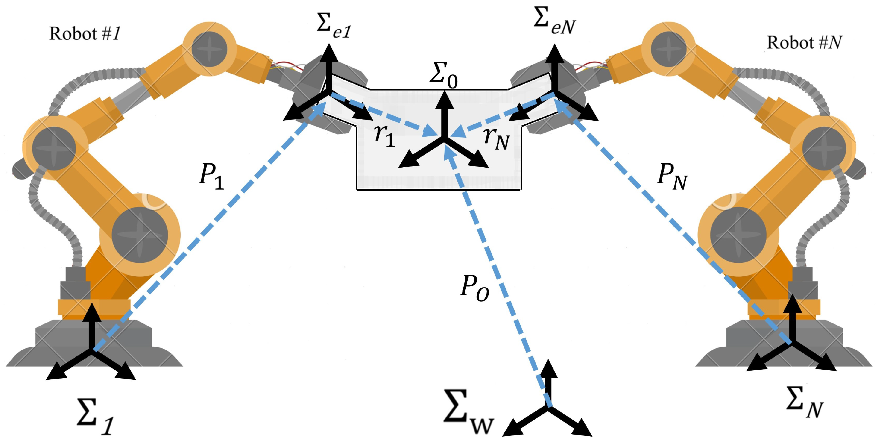
Table 1.
Cooperative robot applications.
| Types | Specific Applications |
|---|---|
| Manufacturing [11,12,13,14,15,16,17,18,19,20,21,22] | CRMs can be used in manufacturing for tasks that requires complex movement such as assembly [19,20]. For example, a team of robot arms can work together to assemble a car engine, with each arm performing a specific task such as tightening bolts or installing parts . Other works such as welding [21] and slabstone installation [22] can be performed by CRMs as well. |
| Warehousing and Logistics [23,24,25,26,27,28,29,30] | They can be used in warehousing and logistics to pick and pack products, move boxes [29,30], transport, and perform other tasks. Multiple arms can work together to increase efficiency and throughput. |
| Construction [31,32] | They can be used in construction to perform tasks such as welding, drilling, and painting. Multiple arms can work together to perform these tasks on a larger scale or in a shorter time frame. |
| Healthcare [33] | They can be used in healthcare to assist with surgeries or other medical procedures, such as nursing. Multiple arms can work together to perform complex procedures, increasing precision and reducing the risk of errors. |
| Agriculture [34,35] | They can be used in agriculture to harvest crops or perform other tasks. Multiple arms can work together to cover more ground and increase efficiency. |
| Aerospace [36,37,38,39,40,41,42,43] | CRMs ability to work alongside human operators, enhance efficiency, and perform tasks that are challenging or unsafe for humans makes them valuable tools in aerospace manufacturing, maintenance, inspection, training, space exploration, and research. Grasping a non-cooperative object [37,42], carrying a load with UAVs [38,41], on-orbit capture, space structure construction and assembly tasks [39], and grasping non-cooperative objects with specific orientations [43]. |
A comprehensive survey for additive manufacturing application is presented in [17].
Table 2.
The advantages and disadvantages of robot modeling in the joint and task space.
| Advantages | Disadvantages | |
|---|---|---|
| Joint-Space Modeling | (1) More suitable for decentralized control algorithms with low communication overhead, scalability, etc. | (1) In some scenarios, like dynamic obstacle avoidance, joint-space control may require complex algorithms and planning to adapt to changing environmental conditions. |
| (2) Joint-space modeling makes it easier to identify and handle singularities. | (2) Complex coordination and synchronization require careful design to ensure overall system objectives are met. | |
| Task (Operational)-Space Modeling | (1) More intuitive (natural) representation for specifying and controlling tasks directly related to end-effector motion, such as moving to a particular position or orientation. | (1) Following a task-space trajectory usually needs an inverse kinematics (IK) solution, which means computational burden, especially if the IK solver is running an optimization. |
| (2) Often, the unified model in task space is suitable for centralized control implementation with better-coordinated decision making. | (2) Task-space modeling and control may lead to a loss of direct control over individual joints, making it less suitable for tasks that require precise manipulation at the joint level. |
Table 3.
Modeling Cooperative Robot Manipulators in the Literature. ✓ indicates the presence of characteristic and × indicates the absence of characteristic.
Table 3.
Modeling Cooperative Robot Manipulators in the Literature. ✓ indicates the presence of characteristic and × indicates the absence of characteristic.
| Reference * | Joint/Task-Space Modeling | Known Payload Model | Known Robot Parameters | Disturbance |
|---|---|---|---|---|
| [54,67] | Task | × | ✓ | × |
| [57] | Task | ✓ | ✓ | ✓ |
| [52,64] | Task | × | ✓ | ✓ |
| [55,76] | Task | ✓ | × | × |
| [29,77,78,79,80] | Joint | ✓ | × | ✓ |
| [56,81,82] | Joint | × | × | ✓ |
| [21,37,59,60,72,83,84,85,86] | Task | × | × | × |
| [87] | Task | × | ✓ | × |
| [88,89] | Joint | × | ✓ | × |
| [74,90,91,92,93,94,95] | Joint | × | × | × |
| [20,22,40,66,75,96,97,98,99,100,101,102,103,104,105,106,107] | Task | ✓ | ✓ | × |
| [51,53,62,65,69,70,73,82,98,107,108,109,110,111,112,113,114,115,116,117,118,119,120,121,122,123,124,125,126,127] | Joint | ✓ | ✓ | × |
* Note that certain references may appear more than once, suggesting that the control scheme has been applied in various contexts or spaces.
Disclaimer/Publisher’s Note: The statements, opinions and data contained in all publications are solely those of the individual author(s) and contributor(s) and not of MDPI and/or the editor(s). MDPI and/or the editor(s) disclaim responsibility for any injury to people or property resulting from any ideas, methods, instructions or products referred to in the content. |
© 2023 by the author. Licensee MDPI, Basel, Switzerland. This article is an open access article distributed under the terms and conditions of the Creative Commons Attribution (CC BY) license (https://creativecommons.org/licenses/by/4.0/).
Share and Cite
MDPI and ACS Style
Ghorbanpour, A. Cooperative Robot Manipulators Dynamical Modeling and Control: An Overview. Dynamics 2023, 3, 820-854. https://doi.org/10.3390/dynamics3040045
AMA Style
Ghorbanpour A. Cooperative Robot Manipulators Dynamical Modeling and Control: An Overview. Dynamics. 2023; 3(4):820-854. https://doi.org/10.3390/dynamics3040045
Chicago/Turabian StyleGhorbanpour, Amin. 2023. "Cooperative Robot Manipulators Dynamical Modeling and Control: An Overview" Dynamics 3, no. 4: 820-854. https://doi.org/10.3390/dynamics3040045