Unraveling Soft Squeezing Transformations in Time-Variant Elastic Fields

Abstract

Quantum squeezing, an intriguing phenomenon that amplifies the uncertainty of one variable while diminishing that of its conjugate, may be studied as a time-dependent process, with exact solutions frequently derived from frameworks grounded in adiabatic invariants. Remarkably, we reveal that exact solutions can be ascertained in the presence of time-variant elastic forces, eschewing dependence on invariants or frozen eigenstate formalism. Delving into these solutions as an inverse problem unveils their direct connection to the design of elastic fields, responsible for inducing squeezing transformations onto canonical variables. Of particular note is that the dynamic transformations under investigation belong to a class of gentle quantum operations, distinguished by their delicate manipulation of particles, thereby circumventing the abrupt energy surges commonplace in conventional control protocols.

1. Introduction

In the fascinating domain of quantum mechanics, one encounters the remarkable phenomenon of squeezing, where the uncertainty tied to a canonical variable diminishes, while that of its conjugate partner swells. This delicate balance between conjugate variables emerges from the grounds of Heisenberg’s uncertainty principle, which prescribes a minimal boundary on the product of their uncertainties, granted that we confine ourselves to a realm where high-energy scales do not warrant further adjustments [1].

In light of this understanding, within the realm of quantum measurements, the uncertainty attached to a particular observable bears the responsibility for any deviations from the intended value—assuming the experimentalist refrains from inadvertently compromising the measurement through extraneous factors. Nevertheless, these imperfections can be ameliorated by attenuating the uncertainty to near-arbitrary levels, albeit at the cost of amplifying the uncertainty of the observable’s counterpart. Such an interplay transcends the familiar position and momentum duality, manifesting itself in other pairs encompassing the spin components of particles or the polarisations of light, among others.

It is precisely this versatile nature of quantum squeezing that has ignited immense interest in its exploration, with researchers drawn to its deep-seated ramifications and promising applications in diverse arenas ranging from quantum information [2] to precision measurements in quantum metrology [3,4,5,6,7,8,9] and quantum teleportation [10]. Even beyond the confines of our current understanding, advancements are being made to measure elusive phenomena, such as dark matter [11].

As we embark on a journey to explore quantum squeezing within the context of time-variant elastic fields, it becomes essential to embrace the Heisenberg picture of quantum mechanics. In contrast to the Schrödinger picture, which accentuates the evolution of the state vector, the Heisenberg picture proffers a complementary description, placing emphasis on the temporal progression of operators, in our case, in the presence of a time-dependent Hamiltonian. This subtle yet profound shift in perspective permits us to unravel squeezing transformations and the mechanisms that underpin them more effectively, which is the aspiration of our investigation.

Despite the abundance of theoretical frameworks that have emerged to explore the intricate facets of time-dependent problems [12,13,14,15,16,17,18,19], our approach diverges from the adiabatic invariants doctrine. In a prior groundbreaking revelation [20], Mielnik demonstrated that the time-evolution problem, characterised by quadratic Hamiltonians endowed with fluctuating elastic forces, admits exact solutions. Intriguingly, these solutions are rooted in a profound understanding of the symmetries embedded within the problem. In this work, we shall continue these solutions to inspect their role in shaping squeezing transformations, and more specifically in fostering the kind of fields that cultivate such linear transformations.

Furthermore, as we shall show, the exact solutions are intimately entwined with the character of the elastic field. This association constitutes an aspect of an inverse problem, in which, upon obtaining an exact solution, the driving field may be meticulously designed. In a reciprocal manner, when provided with an elastic field, one can integrate the system to unveil the corresponding exact solution. This versatility inherent in the method permits us to infuse, with remarkable freedom, any driving elastic force to attain the desired outcome. Such adaptability ensures that we can manipulate the system under the influence of forces that desist from unsettling the particles to the point of dismantling their configuration.

Our work unfolds as follows: In Section 2, we introduce the class of quadratic Hamiltonians equipped with explicit time dependency that underpin our investigation. Section 3 delves into the exact solutions to the time-dependent problem, shedding light on their constraints and implications. Section 4 and Section 5 offer succinct examples of the engineering of designing driving pulses, as well as the inventive squeezing operations that can be fashioned from them. Finally, in Section 6, we present the culminating insights of our work, exposing the limitations and unresolved problems that have emerged from our endeavours.

2. A Classical–Quantum Dynasty of Hamiltonians

Our exploration commences with the family of dimensionless, non-relativistic, quadratic Hamiltonians, each graced with a time-dependent elastic field, herein denoted as $\beta \left(t\right)$. This scenario allows us to express the Hamiltonian for a pair of conjugate variables, q and p, in a rather elementary form:

$$H\left(t\right)=\frac{1}{2}(p^2+\beta \left(t\right)q^2),$$

(1)

where the particle’s mass m and the action constant ℏ are henceforth rendered as unity.

While our exposition shall be nestled in a dimensionless framework, the transition back to physical units can be achieved by adhering to the following relations:

$$p=\frac{p^{\prime }}{\sqrt{\hslash }}=\widehat{p}\sqrt{\frac{T}{\hslash m}},q=\frac{q^{\prime }}{\sqrt{\hslash }}=\widehat{q}\sqrt{\frac{m}{\hslash T}}.$$

(2)

In these relations, $\widehat{p}$ and $\widehat{q}$ denote canonical observables, $p^{\prime }$ and $q^{\prime }$ are both expressed in square root of action units, and T stands as an arbitrary time scale. Consequently, our dimensionless time, t, is expressed as $t=\tau /T$, with $\tau$ representing the time within the frame of reference where the system dwells.

The latter Hamiltonian yields the very same equations of motion for both classical and quantum domains. In the absence of spin, each unitary evolution operator $U(t,t_0)$ in ${\mathcal{L}}^2\left(\mathbb{R}\right)$ generated by the Hamiltonian (1) is wholly determined by the corresponding canonical transformation $H\left(t\right)$ poses [21]. Consequently, the flow generated by $H\left(t\right)$ exhibits striking similarities in both classical and quantum regimes, inspiring further scrutiny of the quantum counterparts of classical trajectories.

Our exposition, in a sense, is devoted to this last pursuit, albeit with a focus on a family of unitary quantum operations that induce the amplification ($\lambda$) or squeezing ($1/\lambda$) of canonical pairs over time. This approach is analogous to that of squeezed states, but instead of directly depicting such states, we study the dynamical operations that give rise to unitary transformations of the form $q\to \lambda q$ and $p\to p/\lambda$. For notable examples in this direction, the reader may refer to [22,23].

With the dimensionless convention in place, the time evolution of the $q,p$ pair is governed by the Hamiltonian (1), and follows the equations of motion given below:

$$\frac{\mathrm{d}q}{\mathrm{d}t}=\frac{1}{\mathrm{i}}[q,H\left(t\right)]=p,\frac{\mathrm{d}p}{\mathrm{d}t}=\frac{1}{\mathrm{i}}[p,H\left(t\right)]=-\beta \left(t\right)q,$$

(3)

where $\mathrm{i}=\sqrt{-1}$. One immediately notes that these equations of motion bear an obvious resemblance in their structure to the classical Hamilton equations: $\mathrm{d}q/\mathrm{d}t=\partial H/\partial p$ and $\mathrm{d}p/\mathrm{d}t=-\partial H/\partial q$.

Letting $Q={(q,p)}^{⊺}$, we can express the system of Equation (3) in a concise and advantageous form:

$$\frac{\mathrm{d}Q}{\mathrm{d}t}=\Lambda \left(t\right)Q,\Lambda \left(t\right)=\left(\begin{array}{cc}0& 1\\ -\beta \left(t\right)& 0\end{array}\right),Q\left(t_0\right)=Q_0={(q_0,p_0)}^{⊺},$$

(4)

this notation serves a particular purpose of ours. In the Heisenberg picture, the time evolution of an observable Q, from an initial time $t_0$ to a given time t, can be expressed as the unitary conjugation of $Q_0$ by the evolution operator $U(t,t_0)$, namely

$$Q\left(t\right)=U^{†}(t,t_0)Q_{0}U(t,t_0)=u(t,t_0)Q_0,$$

(5)

here, $u(t,t_0)$ denotes a dimensionless evolution matrix which is an element of the symplectic group, in our case Sp (2, $\mathbb{R}$).

Both Equations (4) and (5) provide insight into how an observable Q evolves from $t_0$ to t. Consequently, by differentiating (5) with respect to t and substituting into (4), we derive the evolution equation for $u(t,t_0)$:

$$\frac{\mathrm{d}u(t,t_0)}{\mathrm{d}t}=\Lambda \left(t\right)u(t,t_0),u(t_0,t_0)=\mathbb{I},$$

(6)

Since the matrix $u(t,t_0)$ contains complete information about the system’s motion, it is possible to leverage it for various purposes, such as propagating the wave function or even expressing it in terms of the entries of $u(t,t_0)$. Further details can be found in Section 5.

Moreover, the symplectic structure ingrained in $u(t,t_0)$ holds the key to classifying the motion generated by (1), which has been nicely shown in [24,25]. By denoting $\Gamma =Tru(t,t_0)$, it becomes apparent that $u(t,t_0)$ possesses three distinct sets of eigenvalues, computed through the formula $\kappa =\frac{1}{2}(\Gamma \pm \sqrt{{\Gamma }^2-4})$. Each set characterises a unique class of motion:

I

When $|\Gamma |$ > 2, the eigenvalues $\kappa$ become real, thereby causing unstable motion. This regime is conducive to the squeezing phenomena of canonical operators, $a^{†}$ and a, defined by the eigenvectors of $u(t,t_0)$.

II

When $|\Gamma |$ = 2, the eigenvalues $\kappa$ are also real. However, unlike in regime I, these eigenvalues may lead the motion to stable regimes as well.

III

When $|\Gamma |$ < 2, the eigenvalues $\kappa$ are complex, and the motion is (oscillatory) stable. For a periodic process of length T, $u(t,t_0)=u(T+t,t_0)$ will define global operators $a^{†}$ and a. This regime permits quantum operations for the confinement of particles, such as Paul traps [26].

The pre-eminent role of $\Gamma$ in the above classification is a natural consequence of the symplectic structure inherent in $u(t,t_0)$. Therefore, it is reasonable to surmise that $\Gamma$ and $\beta \left(t\right)$ are intertwined to some degree. Indeed, the particular form of the pulse dictated by $\beta \left(t\right)$ is ultimately responsible for the resulting class of motion. To illustrate this point, let us consider the case where $\beta \left(t\right)$ is a constant value of ${\omega }^2$. In this scenario, the integration of (6) is straightforward and yields $\Gamma =2cos\left(\omega t\right)$. Depending on the magnitude of $\Gamma$ (and of course of $\omega$), the system demonstrates either the common oscillatory motion associated with class III, or, as $\Gamma$ nears the parametric resonance threshold, motion akin to a free particle in class II. We will delve into the relationship between $\Gamma$ and $\beta \left(t\right)$ in greater detail in Section 3.

3. Time Evolution without Adiabatic Invariants

In 2013, Mielnik [20] made a remarkable mathematical discovery regarding the system of differential Equation (6). Specifically, he noted that exact solutions can be obtained for this system, presuming the elastic field $\beta \left(t\right)$ is symmetric over the interval of integration. We will see that these exact solutions provide us with valuable insight into the simplest cases of the evolutive problem represented by (6). As well, it is worth noting that these solutions offer an opportunity to design control operations by smoothly varying the steering fields, nearly adiabatically, without any requirement for invariant formalism [13,15]. In addition, these solutions are inherently linked to $\beta \left(t\right)$ itself, allowing one to either evolve $u(t,t_0)$ by means of an elastic pulse or design the elastic pulse required for specific purposes. The latter strategy, in particular, may have wide-ranging implications in fields such as quantum computing, quantum sensing, and metrology, where it is necessary to manipulate particles in order to achieve a desired state.

Suppose we consider a symmetric pulse $\beta \left(t\right)$ with respect to the centre of the operation interval $[-t,t]$. We see that in this interval the unitary operators $U(t,-t)$ do satisfy $\mathrm{d}U(t,-t)/\mathrm{d}t=\left[H\right(t\left)U\right(t,-t)+U(t,-t\left)H\right(t\left)\right]/2\mathrm{i}$, because the quadratic Hamiltonian (1) satisfies $H\left(t\right)=H(-t)$. The system described by (6) then takes the form

$$\frac{\mathrm{d}u(t,-t)}{\mathrm{d}t}=\frac{1}{2}\left(\Lambda \left(t\right)u(t,-t)+u(t,-t)\Lambda \left(t\right)\right)u(-t,-t)=\mathbb{I},$$

(7)

using $\Lambda \left(t\right)$ as defined in (4), we can explicitly write the former equation in terms of $\beta \left(t\right)$ and the entries of $u(t,-t)$:

$$\frac{\mathrm{d}}{\mathrm{d}t}\left(\begin{array}{cc}{u}_{11}& u_{12}\\ u_{21}& u_{22}\end{array}\right)=\frac{1}{2}(u_{21}-\beta \left(t\right)u_{12})\mathbb{I}+\frac{\Gamma }{2}\Lambda \left(t\right).$$

(8)

Upon examination, we quickly observe that the diagonal elements on the left-hand side both share the same differential equation, namely, $\mathrm{d}{u}_{11}/\mathrm{d}t=\mathrm{d}{u}_{22}/\mathrm{d}t=(u_{21}-\beta \left(t\right)u_{12})/2$. Consequently, it follows that $u_{11}=u_{22}=\Gamma /2$. Now, here comes the clever part. If we insert an almost arbitrary analytical function $u_{12}\equiv \theta \left(t\right)\in \mathbb{R}$, we can also observe from (8) that $\dot{\theta }\left(t\right)\equiv \mathrm{d}\theta \left(t\right)/\mathrm{d}t=\Gamma /2$.

In turn, we shall deduce the form of $u_{21}$ based on the aforementioned information, and recalling that $u(t,-t)\in Sp(2,\mathbb{R})$. Because $detu(t,-t)={\dot{\theta }}^2\left(t\right)-\theta \left(t\right)u_{21}=1$, we solve $u_{21}$ from here to finally obtain $({\dot{\theta }}^2\left(t\right)-1)/\theta \left(t\right)$, which implies that the evolution matrix $u(t,-t)$ has the explicit form

$$u(t,-t)=\left(\begin{array}{cc}\dot{\theta }\left(t\right)& \theta \left(t\right)\\ \frac{{\dot{\theta }}^2\left(t\right)-1}{\theta \left(t\right)}& \dot{\theta }\left(t\right)\end{array}\right).$$

(9)

With the preceding discussion, the reader may be able to anticipate the relationship that exists between $\beta \left(t\right)$ and the trace $\Gamma$ of the evolution matrix. For the time-independent case, as shown in the example at the end of Section 2, this relationship becomes evident. However, in the time-dependent case, we need to provide a detailed derivation to explicitly establish this connection. Fortunately, this task is not arduous, and we shall undertake it now.

The path to unlocking the relation subtended between $\beta \left(t\right)$ and $\theta \left(t\right)$ lies in the differential equation for the entry $u_{21}$ in (8). Through careful examination, we uncover the expression $\mathrm{d}{u}_{21}/\mathrm{d}t=-\beta \left(t\right)\Gamma /2=-\dot{\theta }\left(t\right)\beta \left(t\right)=\mathrm{d}[({\dot{\theta }}^2\left(t\right)-1)/\theta \left(t\right)]/\mathrm{d}t$. A rearrangement of terms and a simplification of the resulting expression brings the connection between $\beta \left(t\right)$ and $\theta \left(t\right)$:

$$\beta \left(t\right)=-\frac{2\ddot{\theta }\left(t\right)\theta \left(t\right)-{\dot{\theta }}^2\left(t\right)+1}{{\theta }^2\left(t\right)}.$$

(10)

In this way, Mielnik’s discovery entails that $\theta \left(t\right)$ is indeed an exact solution to the evolution problem (7), while simultaneously enabling us to tackle an inverse problem of sorts: should $\beta \left(t\right)$ be known, we may infer $\theta \left(t\right)$ (cf. Section 4); conversely, given $\theta \left(t\right)$, we may deduce $\beta \left(t\right)$. The interplay between these two functions therefore yields a versatile method for analysing the classes of motion regulated by (7). Yet another avenue to relate $\beta \left(t\right)$ and $\theta \left(t\right)$ lies in the differential equations for $u_{11}=u_{22}$. By simply substituting $({\dot{\theta }}^2\left(t\right)-1)/\theta \left(t\right)$ into $u_{21}$ and performing some straightforward algebraic manipulation, (10) is once again obtained.

An interesting detail warrants our consideration. By suitably rearranging the terms of the expression in (10), we are led to a time-dependent, effective harmonic oscillator, whose frequency is given by $\sqrt{\beta \left(t\right)/2}$, namely,

$$\ddot{\theta }\left(t\right)+\frac{\beta \left(t\right)}{2}\theta \left(t\right)={\eta }_{\mathrm{eff}}(\theta ,\dot{\theta }),$$

(11)

where ${\eta }_{\mathrm{eff}}$ contains nonlinear terms that we interpret as being part of an effective damping component:

$${\eta }_{\mathrm{eff}}(\theta ,\dot{\theta })\equiv \frac{{\dot{\theta }}^2\left(t\right)-1}{2\theta \left(t\right)},$$

(12)

These terms, and of course $\beta \left(t\right)$, shall help in explaining the class of oscillation $\theta \left(t\right)$ undergoes. Is there a regime in which such nonlinear terms are of no importance?

From Equation (9), we can observe that whenever $\theta$ becomes zero at a certain point t, then $\dot{\theta }\left(t\right)$ at the same point must be equal to $\pm 1$. Additionally, we notice that a time-dependent Fourier transform takes place if $\dot{\theta }\left(t\right)$ becomes zero at $t=T$, but ${\theta }_T\equiv \theta \left(T\right)\ne 0$, then

$$u\left(T\right)=\left(\begin{array}{cc}0& {\theta }_T\\ -\frac{1}{{\theta }_T}& 0\end{array}\right),$$

Following the application of this matrix to a pair of conjugate variables, q and p, a transformation of the form $q\to p{\theta }_T$ and $p\to -q/{\theta }_T$ is obtained. In other words, this transformation swaps such two variables and rescales each one with respect to ${\theta }_T$ and its reciprocal. A second application of the same matrix—i.e., fixing $\theta \left(t\right)$—reverts the Fourier transform effect, restoring the variables to their original values. However, suppose now that a similar Fourier transform occurs at a different time $T^{\prime }$ for a function ${\theta }^{\prime }\left(t\right)\ne \theta \left(t\right)$. Then, the composition of two different Fourier transform matrices (or an even number of them) will lead to squeezing transformations (belonging to the class of motion I):

$$\left(\begin{array}{cc}0& {\theta }_T\\ -\frac{1}{{\theta }_T}& 0\end{array}\right)\left(\begin{array}{cc}0& {\theta }_{T^{\prime }}^{\prime }\\ -\frac{1}{{\theta }_{T^{\prime }}^{\prime }}& 0\end{array}\right)=\left(\begin{array}{cc}\lambda & 0\\ 0& \frac{1}{\lambda }\end{array}\right),\lambda \equiv -\frac{{\theta }_T}{{\theta }_{T^{\prime }}^{\prime }},$$

(13)

specifically, this results in linear transformations of the form $q\to \lambda q$ and $p\to p/\lambda$, wherein one variable is amplified at the expense of squeezing the other or vice versa.

3.1. What If $\beta \left(t\right)$ Is Odd?

Squeezing phenomena have been observed to occur in intervals where $\beta \left(t\right)$ is not symmetric with respect to the centre of the operation interval [27]. Therefore, upon acquiring the elastic field $\beta \left(t\right)$ utilising (10), the integration of Equation (6) is required over an interval with a non-coinciding centre compared to that of $\beta \left(t\right)$. This analysis prompts the inquiry of whether a reformation is warranted for a $\beta \left(t\right)\ne \beta (-t)$ spanning the entire operational interval.

This is particularly relevant if we consider the steering force to be a time-dependent, magnetic induction field, as it is crucial to note that the case where $-\beta \left(t\right)=\beta (-t)$ cannot even be considered. If such a condition were to hold, it would lead to imaginary forces, which are physically impossible. Upon closer examination, let us consider the Hamiltonian $H\left(t\right)={(\mathbf{p}-\mathbf{A}(\mathbf{x},t))}^2/2$, where $\mathbf{A}(\mathbf{x},t)$ represents the vector potential—recalling that we adopt the convention of setting all physical constants to unity. We shall choose a symmetric gauge in which $\mathbf{A}(\mathbf{x},t)=\left[\mathbf{B}\right(\mathbf{x},t)\wedge \mathbf{x}]/2$. When we assume the magnetic induction field is oriented along the $Oz$ direction, we have $\mathbf{B}(\mathbf{x},t)=B\left(t\right){\mathbf{e}}_z$. Thus, the identification of $\beta \left(t\right)=B^2\left(t\right)$ elucidates the requirement for $\beta \left(t\right)$ to be even when the driving force originates from a magnetic field [28].

However, in the case of a scalar field, such as the electric potential used in Paul traps [26], the elastic field $\beta \left(t\right)$ is directly proportional to the applied voltage $\varphi \left(t\right)$ on the surfaces of the trap, see Section 6. In this context, it is possible to consider the case where $-\beta \left(t\right)=\beta (-t)$ without impediment. We will explore this case further below. However, first, to prevent any possible confusion between the distinct exact solutions for an elastic field of this type and those described in Equation (10), let us introduce some notation. We shall use the symbol ∗ to differentiate between these solutions.

By assuming that $-{\beta }_{\ast }\left(t\right)={\beta }_{\ast }(-t)$, the Hamiltonian (1) shall satisfy $-H_{\ast }\left(t\right)=H_{\ast }(-t)$, while the unitary evolution operators hold $\mathrm{d}{U}_{\ast }(t,-t)/\mathrm{d}t=[H_{\ast }\left(t\right)U_{\ast }(t,-t)-U_{\ast }(t,-t)H_{\ast }\left(t\right)]/2\mathrm{i}$. With these premises, we may proceed to state the initial value problem (6) as

$$\frac{\mathrm{d}{u}_{\ast }(t,-t)}{\mathrm{d}t}=\frac{1}{2}\left({\Lambda }_{\ast }\left(t\right)u_{\ast }(t,-t)-u_{\ast }(t,-t){\Lambda }_{\ast }\left(t\right)\right)u_{\ast }(-t,-t)\ne \mathbb{I},$$

(14)

or explicitly:

$$\frac{\mathrm{d}}{\mathrm{d}t}{\left(\begin{array}{cc}{u}_{11}& u_{12}\\ u_{21}& u_{22}\end{array}\right)}_{\ast }=\frac{1}{2}{(u_{21}+\beta \left(t\right)u_{12})}_{\ast }\left(\begin{array}{cc}1& 0\\ 0& -1\end{array}\right)+\frac{{(u_{22}-u_{11})}_{\ast }}{2}{\Lambda }_{\ast }\left(t\right).$$

With proper attention, we notice that the diagonal elements on the left-hand side satisfy the same differential equation, up to a sign. Therefore, it follows that ${\left(u_{11}\right)}_{\ast }=-{\left(u_{22}\right)}_{\ast }=-{\dot{\theta }}_{\ast }\left(t\right)$, and as a consequence, the matrix $u_{\ast }(t,-t)$ corresponding to a given ${\beta }_{\ast }\left(t\right)$ will be traceless. This, in turn, assures that the motion will always be of class III, although the even composition of these matrices does not necessarily follow this pattern.

Furthermore, as previously discussed, we recall that $u_{\ast }(t,-t)$ is an element of $Sp(2,\mathbb{R})$, and thus its determinant is unity. From this condition, we can determine the form that the entry ${\left(u_{22}\right)}_{\ast }$ will take, leading us to the following expression for $u_{\ast }(t,-t)$:

$$u_{\ast }(t,-t)=\left(\begin{array}{cc}-{\dot{\theta }}_{\ast }\left(t\right)& {\theta }_{\ast }\left(t\right)\\ -\frac{{\dot{\theta }}_{\ast }^2\left(t\right)+1}{{\theta }_{\ast }\left(t\right)}& {\dot{\theta }}_{\ast }\left(t\right)\end{array}\right),$$

(15)

Thus, we establish a relation between ${\beta }_{\ast }\left(t\right)$ and the exact solution ${\theta }_{\ast }\left(t\right)$, namely,

$${\beta }_{\ast }\left(t\right)=-\frac{2{\ddot{\theta }}_{\ast }\left(t\right){\theta }_{\ast }\left(t\right)-{\dot{\theta }}_{\ast }^2\left(t\right)-1}{{\theta }_{\ast }^2\left(t\right)}.$$

(16)

Upon comparing Equations (10) and (16) for $\beta \left(t\right)$ and ${\beta }_{\ast }\left(t\right)$, we notice that they differ solely in the sign of the third term. In fact, similar to our interpretation in (11), the nonlinear terms can be viewed as constituents of an effective force that propels the time-dependent harmonic oscillator:

$${\ddot{\theta }}_{\ast }\left(t\right)+\frac{{\beta }_{\ast }\left(t\right)}{2}{\theta }_{\ast }\left(t\right)={\eta }_{\mathrm{eff}\ast }({\theta }_{\ast },{\dot{\theta }}_{\ast }),$$

(17)

where

$${\eta }_{\mathrm{eff}\ast }({\theta }_{\ast },{\dot{\theta }}_{\ast })\equiv \frac{{\dot{\theta }}_{\ast }^2\left(t\right)+1}{2{\theta }_{\ast }\left(t\right)}.$$

(18)

In contrast to the exact solutions presented in (10), it is necessary to carefully consider the conditions that ${\theta }_{\ast }\left(t\right)$ must satisfy for the initial value problem (14). In order for these solutions to generate a corresponding well-behaved ${\beta }_{\ast }\left(t\right)$—or conversely, for any well-behaved $\beta \left(t\right)$ to have a field ${\theta }_{\ast }\left(t\right)$ that possesses no singularities—it is essential that ${\theta }_{\ast }\left(t\right)$ does not vanish at any time t, even at those times at which ${\dot{\theta }}_{\ast }\left(t\right)$ becomes zero. In the event that this latter condition is met, $u_{\ast }(t,-t)$ will become a Fourier transform matrix.

However, these solutions would induce a Fourier transform at the very beginning of the interval of operation, regardless of any prior knowledge of the conjugate variable trajectories. In such scenarios, the particle would receive streams of energy significant enough to disrupt it from its original state, with a high probability of losing any control over it. Yet, since the aim of our discussion is to study quantum operations that exhibit soft transitions to a given target, we shall limit our discussion to symmetric $\beta \left(t\right)$ fields with respect to the centre of the interval of manipulation.

4. Shaping Elastic Fields like a Blacksmith

According to the method we have surveyed in the previous section, the flexibility of the approach relies, in addition to the specifics, on the freedom to choose a function $\theta \left(t\right)$ for designing an elastic driving field $\beta \left(t\right)$. Conversely, given a $\beta \left(t\right)$, one can imagine the corresponding $\theta \left(t\right)$, which is the exact solution to the initial value problem described by Equation (6). In general, the latter presents a formidable challenge, often demanding numerical efforts, with exact solutions not invariably assuming a closed form. We shall introduce elementary arguments with the intent to streamline the solvability of Equation (10), whether in its direct or inverse form.

The simplest model to consider is when we set $\beta \left(t\right)={\omega }^2$, where $\omega$ is a real constant. In this case, Equation (10) has an exact solution given by $\theta \left(t\right)=sin\left(\omega t\right)/\omega$. This solution breaks the nonlinearities in the effective damping terms, resulting in ${\eta }_{\mathrm{eff}}(\theta ,\dot{\theta })=-{\omega }^2\theta \left(t\right)/2$. As a result, Equation (11) is reduced to the familiar form $\ddot{\theta }\left(t\right)+{\omega }^2\theta \left(t\right)=0$. Therefore, for this exact solution, the evolution matrix $u(t,-t)$ will become a symplectic rotation matrix:

$$u(t,-t)=\left(\begin{array}{cc}cos\left(\omega t\right)& \frac{1}{\omega }sin\left(\omega t\right)\\ -\omega sin\left(\omega t\right)& cos\left(\omega t\right)\end{array}\right),$$

(19)

If we allow for the parameter $\omega$ to take values of $n\pi$, where n represents an integer, and restrict our considerations to the interval of operation $[-1,1]$, then the matrix in question facilitates a sequence of transitions, in intervals of length $1/2n$, between a Fourier transform and its inverse. Such a process is characterised by a smoothness which can be observed in the resultant sequences.

Moreover, it should be noted that setting $\beta \left(t\right)=-{\omega }^2$ would lead to a repulsive harmonic oscillator, with the exact solution given by $\theta \left(t\right)=sinh\left(\omega t\right)/\omega$. However, to what degree of validity might this solution aspire? This choice would also eliminate the nonlinearities in the effective damping terms, as ${\eta }_{\mathrm{eff}}(\theta ,\dot{\theta })$ becomes a linear function of $\theta$. For this solution to hold, one could imagine a scenario in the context of electric potentials, where the class of operation can depend on the sign of the applied voltage. It could be stated that the system in question would possess the ability to exhibit either an attractive or repulsive behaviour depending on the steering voltage. Nevertheless, within the realm of real numbers, it appears that no single point exists at which this exact solution could culminate in a Fourier transform matrix for (9). As we commented in Section 3.1, it is not our intention to scrutinise these particular scenarios within the confines of our present discussion. Rather, we shall address such a survey in a separate manuscript. In point of fact, in order to ensure the validity of $\beta \left(t\right)$ for the purposes we seek, we must adhere to the constraints set forth in the following Lemma [20], which summarises the constraints that restrict the arbitrariness of $\theta \left(t\right)$.

Lemma 1.

Given any $\beta \left(t\right)$ exhibiting symmetry with respect to the central point of the interval $t\in [-\tau ,\tau ]$, the function $\theta \left(t\right)$ must maintain continuity and, at a minimum, possess the quality of being three-times differentiable. To ensure that both functions satisfy the necessary conditions for proper definition through Equation (10), these criteria must be met:

• At any time t when $\theta \left(t\right)=0$, then $\mathrm{d}\theta \left(t\right)/\mathrm{d}t=\pm 1$.
• At any time t when $\beta \left(t\right)\ne 0$ and $\theta \left(t\right)\ne 0$ but their derivatives with respect to time both vanish simultaneously, then ${\mathrm{d}}^3\theta \left(t\right)/\mathrm{d}{t}^3=0$.
• At any time t when $\theta \left(t\right)\ne 0$ and $\mathrm{d}\theta \left(t\right)/\mathrm{d}t=0$, the evolution matrix $u(t,-t)$ represents a Fourier transform of the $q,p$ canonical pair at that point.

Proof. 

The conditions numbered 1 and 2 are a direct consequence of Equation (8), which underscores the indispensable requirement that $u_{21}$ must possess a finite value. Moreover, we see from (10) that in case $\dot{\theta }\left(t\right)$ vanishes at a given t, we are led to $2\ddot{\theta }\left(t\right)\theta \left(t\right)=\beta \left(t\right){\theta }^2\left(t\right)-1$, and by differentiating this expression with respect to time the second condition becomes evident. The condition numbered 3 is fulfilled provided the antidiagonal elements of $u(t,-t)$ induce a linear transformation that can be expressed in the form of $q\propto p$ and $p\propto -q$. □

The Inverse Problem Unveiled

The task of selecting an appropriate $\theta \left(t\right)$ that satisfies Lemma 1 necessitates an empirical exploration of functions tailored to the specific control objective. In the subsequent discussion, we will narrow our focus to a particular class of $\theta \left(t\right)$ functions that possess the ability to create vanishing elastic fields at both the beginning and the end of the operating interval. Hence, we allow $\theta \left(t\right)$ to be expressed as

$$\theta \left(t\right)=\sum _{n=0}^{\infty }{a}_{n}sin\left({\omega }_{n}t\right).$$

(20)

With this particular choice, the expression for the elastic field (10) becomes

$$\beta \left(t\right)=\frac{2\left({\sum }_{n=0}^{\infty }{a}_{n}sin\left({\omega }_{n}t\right)\right)\left({\sum }_{n=0}^{\infty }{a}_n{\omega }_n^{2}sin\left({\omega }_{n}t\right)\right)+{\left({\sum }_{n=0}^{\infty }{a}_n{\omega }_{n}cos\left({\omega }_{n}t\right)\right)}^2-1}{{\left({\sum }_{n=0}^{\infty }{a}_{n}sin\left({\omega }_{n}t\right)\right)}^2},$$

(21)

we must judiciously determine the coefficients $a_n$ and the frequencies ${\omega }_n$, basing our search on the conditions specified in the preceding Lemma. In practice, not all of the unknown coefficients will be determined by the imposed conditions; instead, we will be required to have additional free parameters.

Let us examine the first three terms in series (20) and attempt to determine some of the coefficients. To streamline our inspection, we shall concentrate on the operational interval $t\in [-\pi ,\pi ]$, with the angular frequencies ${\omega }_n$ established by the arbitrary choice of $({\omega }_1,{\omega }_2,{\omega }_3)=(1,3,5)$. According to the initial value problem in (6), at the beginning of the operation, we have $\dot{\theta }(-\pi )=1$ and $\theta (-\pi )=0$. By closely scanning, we find that $\dot{\theta }\left(t\right)$ attains zero at $\pm \pi /2$, which implies $\theta (\pm \pi /2)\ne 0$. Consequently, we have $\ddot{\theta }(\pm \pi /2)=-[\beta (\pi /2)\theta (\pm \pi /2)+1/\theta (\pm \pi /2)]/2$. Given these considerations, and by setting $\theta (\pi /2)={\alpha }_1$ and $\ddot{\theta }(\pi /2)={\alpha }_2$, we derive a linear system of equations involving the coefficients $a_1,a_2$, and $a_3$:

$$\left(\begin{array}{ccc}1& 3& 5\\ -1& 1& -1\\ 1& -9& 25\end{array}\right)\left(\begin{array}{c}{a}_1\\ a_2\\ a_3\end{array}\right)=\left(\begin{array}{c}-1\\ {\alpha }_1\\ {\alpha }_2\end{array}\right),$$

(22)

As we resolve the linear system, the three coefficients will be expressed in terms of ${\alpha }_1$ and ${\alpha }_2$, which are to be varied such that $\beta \left(t\right)$ adopts the properties of interest. Notably, ${\alpha }_1$ is connected to the amplitude of the scaling factor within the Fourier transformation process.

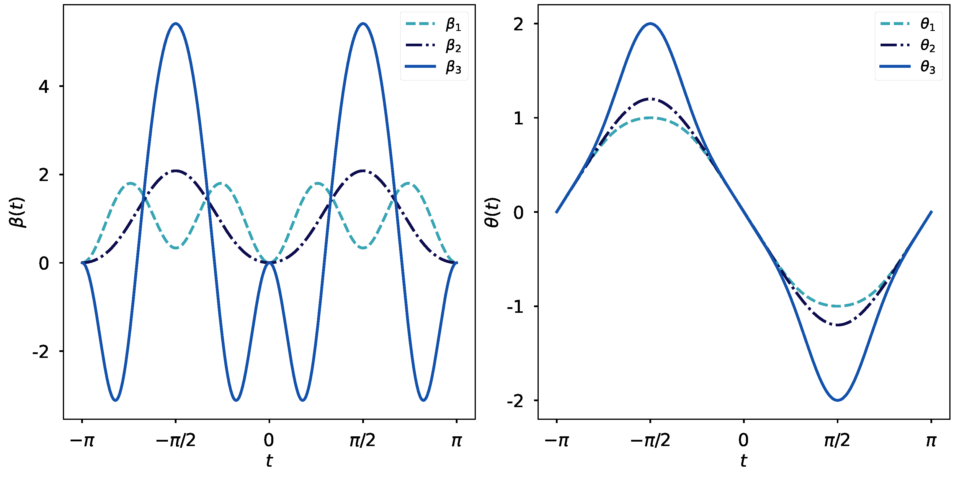
To illustrate the design of the elastic fields with utmost clarity, we have selected different values for the parameters ${\alpha }_1$ and ${\alpha }_2$. As a result, the $\beta \left(t\right)$ fields take shape as depicted in the plots of Figure 1, where the corresponding exact solutions are shown as well. The assortment of values we have selected for ${\alpha }_1$ and ${\alpha }_2$ permit the $\beta \left(t\right)$ fields to vanish softly at the beginning and at the end of the interval $[-\pi ,\pi ]$.

The pulses denoted as ${\beta }_1$ and ${\beta }_2$ persistently display positive values across the entire interval. For these pulses, the parameter ${\alpha }_1$ adopts values of 1 and $6/5$, respectively, while the parameter ${\alpha }_2$ assumes values of $-2/3$ and $-5/3$. Consider a quantum operation constructed by the consecutive combination of these two fields; the outcome at the conclusion of the operational interval would manifest as a squeezing transformation of magnitude $6/5$. Contrastingly, the pulse ${\beta }_3$ portrayed in the figure exhibits a greater magnitude compared to its counterparts. For this particular pulse, the parameters were set as ${\alpha }_1=2$ and ${\alpha }_2=-17/3$. This suggests that the extent of the squeezing effect is intricately linked to the magnitude of the elastic field governing the quantum operation.

5. A Soft Squeezing Engine

We have previously remarked that each individual $\beta \left(t\right)$ pulse depicted in Figure 1 has the attribute to yield a time-dependent Fourier transform at specific instants throughout the operational interval, particularly at the roots of $\dot{\theta }\left(t\right)$. Suppose we identify the precise instances when a Fourier transform occurs for each of these elastic fields. We then construct a quantum operation using two consecutive, distinct $\beta \left(t\right)$ functions, with one following immediately after the other has reached a Fourier transform, as outlined in Equation (13). However, in deviating from this portrayal, the ultimate outcome at the conclusion of the operational interval will manifest as a seamless squeezing transformation, brought forth by the driving fields in question.

In order to more effectively explain the manner in which the smooth squeezing process occurs throughout the operational time interval, we shall first examine the two $\beta \left(t\right)>0$ fields depicted in Figure 1. At this point, the reasoning behind the deliberate simplification in our exposition, by selecting an exact solution $\theta \left(t\right)$ conforming to the function in (20), ought to become apparent. Indeed, it is precisely for the three pulses studied in the preceding section that a Fourier transform arises at odd multiples of $\pi /2$.

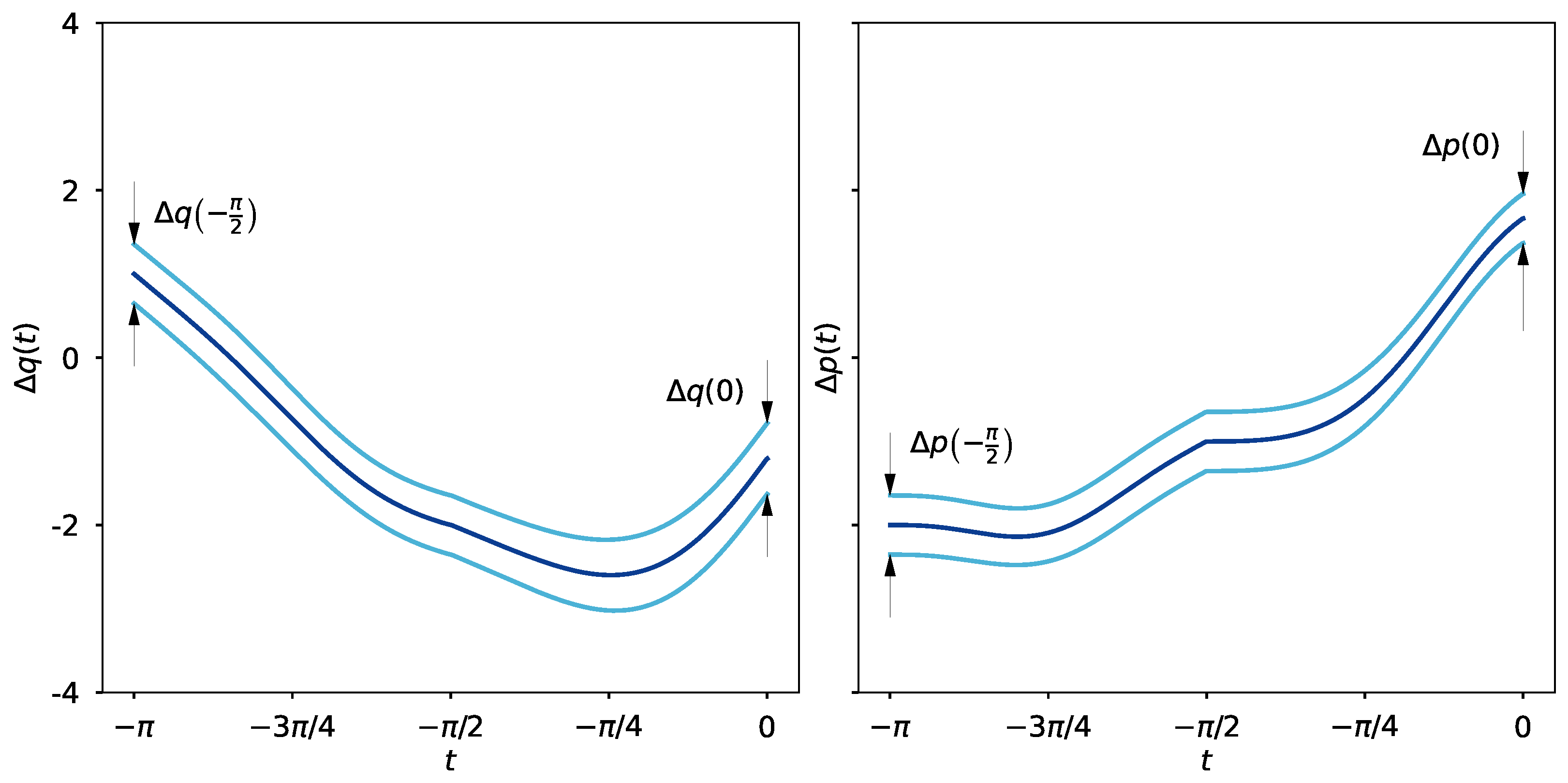
Envision a physical realisation involving a cylindrical solenoid, conceived as a longitudinally aligned coil of wire. In this setup, a time-dependent electric current feeds into the solenoid, which in turn induces a magnetic induction field that permeates the cylinder. By subtly modulating this current—and thus the magnetic field—we can generate the pulses ${\beta }_1$ and ${\beta }_2$ in a precisely controlled manner, facilitating the desired dynamical operation. Such an operation initiates with the pulse denoted by ${\beta }_1$, immediately succeeded by the pulse ${\beta }_2$, both within the operational interval $[-\pi ,-\pi /2]\cup [-\pi /2,0]$. Under the presumption that the initial conditions at $t=-\pi$ are $q(-\pi )=1$ and $p(-\pi )=-2$, the temporal development of the squeezing effect imposed onto the canonical pair shall display a characteristic akin to that delineated in Figure 2, achieving a squeezing effect of magnitude $\left|\lambda \right|=6/5$. Specifically, this scenario employs the solenoid’s magnetic field to enact a soft squeezing operation. The class of quantum operations achievable via this method is termed soft, due to their nature of introducing small, controlled modifications to the system’s state.

Moreover, analogous to the process characterised in Equation (13), the intrinsic machinery governing this continuous landscape shall likewise manifest as the successive employment of matrices belonging to $Sp(2,\mathbb{R})$:

$$\left(\begin{array}{cc}{\dot{\theta }}_1& {\theta }_1\\ \frac{{\dot{\theta }}_1^2-1}{{\theta }_1}& {\dot{\theta }}_1\end{array}\right)\left(\begin{array}{c}q\left(-\pi \right)\\ p\left(-\pi \right)\end{array}\right)=\left(\begin{array}{c}q\left(-\frac{\pi }{2}\right)\\ p\left(-\frac{\pi }{2}\right)\end{array}\right)\to \left(\begin{array}{cc}{\dot{\theta }}_2& {\theta }_2\\ \frac{{\dot{\theta }}_2^2-1}{{\theta }_2}& {\dot{\theta }}_2\end{array}\right)\left(\begin{array}{c}q\left(-\frac{\pi }{2}\right)\\ p\left(-\frac{\pi }{2}\right)\end{array}\right)=\left(\begin{array}{c}q\left(0\right)\\ p\left(0\right)\end{array}\right),$$

which shall generate the subtle transition towards a squeezing transformation through the sequential employment of two elastic fields that smoothly vanish at the commencement and termination of their respective intervals of influence.

Both q and p shall describe semiclassical trajectories, accompanied by their corresponding uncertainty shadows—which we will discuss shortly—as depicted in Figure 2. The instance under consideration exemplifies that the uncertainties associated with q and p undergo, respectively, amplification and squeezing at the operation’s culmination to a moderate degree—a direct ramification of the applied field’s nuanced strength. It becomes patently clear that each uncertainty belt advances in mutual correspondence with its associated trajectory, a guarantee conferred by the symplectic structure embodied in the matrices $u(t,t_0)$.

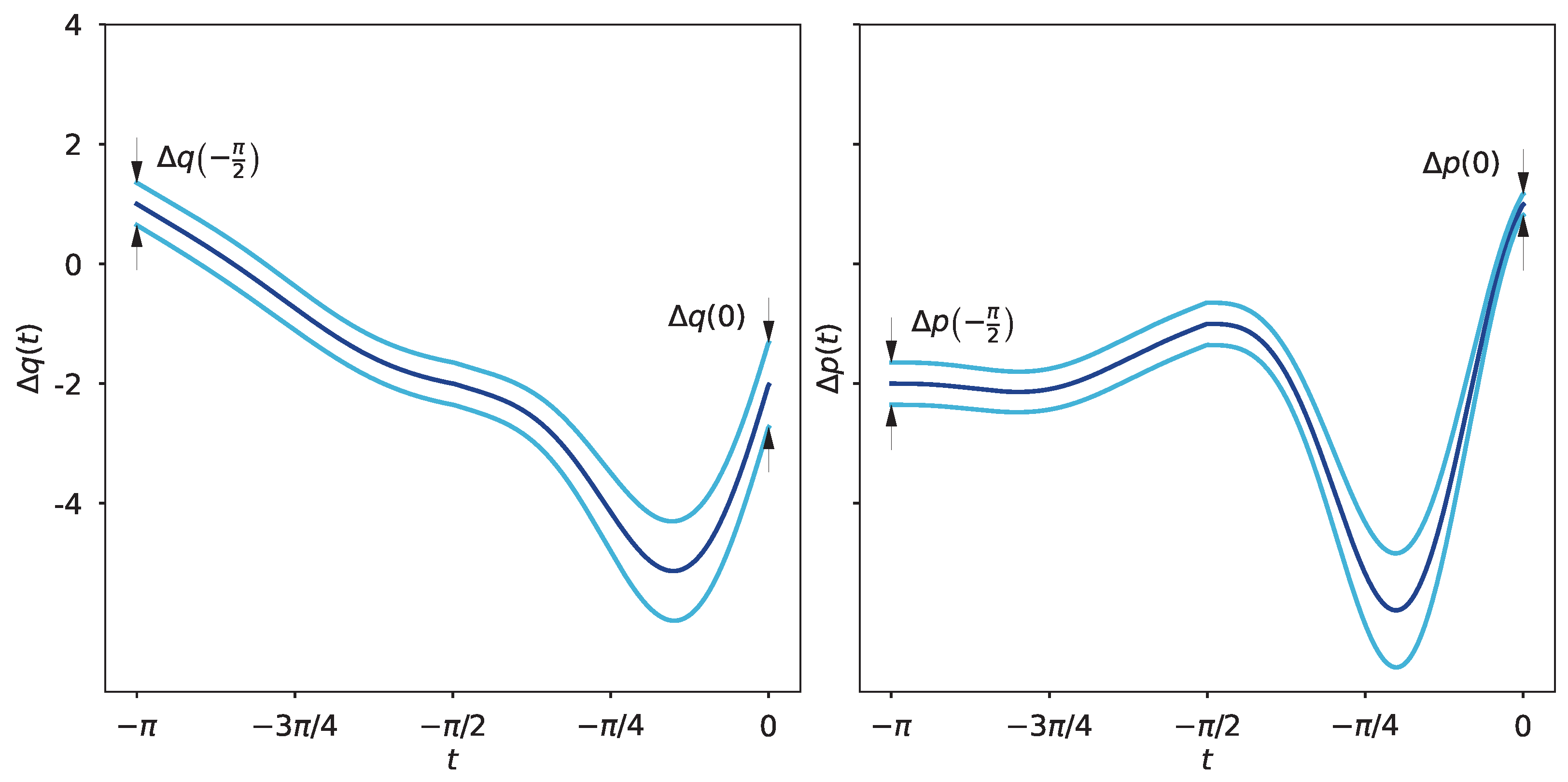
A second example, stemming from the pulses in Figure 1, merits inclusion in our discussion. We shall proceed as before, but this time our focus will be on a squeezing operation comprising pulses ${\beta }_1$ and ${\beta }_3$. A physical realisation involving these elastic forces would necessitate the absence of a driving magnetic induction field, relying solely on the application of a time-varying electric potential, as commonly encountered in quadrupole ion traps of hyperbolic geometry. To facilitate comparison with our previous example, we shall maintain the same initial conditions and operational interval. The temporal progression of the squeezing transformation can be discerned in Figure 3, wherein the extent of the compression of uncertainty $\Delta p\left(t\right)$ is evident, being reduced by a factor of 2—the value of the parameter ${\alpha }_1$ being assumed in order to generate pulse ${\beta }_3$.

Evolving Uncertainty Shadows

The matrices $u(t,t_0)$ facilitate not solely the evolution of the canonical pair and other observables, but that of the wave function itself. To elucidate this notion, let us consider a Gaussian wave function residing in the domain of ${\mathcal{L}}^2\left(\mathbb{R}\right)$. Presume that, in the coordinate representation, the wave function is situated at $x=q_0$ at the initial instant in the operational time:

$$\Psi (x,0)={\left(\frac{1}{2\pi {(\Delta q)}^2}\right)}^{\frac{1}{4}}exp\left(\mathrm{i}{p}_0(x-q_0)\right)exp\left(-\frac{{(x-q_0)}^2}{4{(\Delta q)}^2}\right),$$

(23)

where ${(\Delta q)}^2$ is the uncertainty of the variable q. To determine the value it assumes, we simply employ the customary Robertson–Schrödinger expression for the uncertainty linked to an observable $\mathcal{O}$, namely ${(\Delta \mathcal{O})}^2=\langle {\mathcal{O}}^2\rangle -{\langle \mathcal{O}\rangle }^2$, where $\langle ·\rangle$ symbolises the expected value. We see that, at the inception of the operational time, the uncertainties for the canonical pair under scrutiny satisfy ${(\Delta q)}^2={(\Delta p)}^2=1/2$. Indeed, in light of the time evolution of variables q and p being dictated by the evolution matrix of form (6), it requires minimal exertion to ascertain the evolved uncertainties:

$${(\Delta q\left(t\right))}^2=\frac{1}{2}\left({\dot{\theta }}^2\left(t\right)+{\theta }^2\left(t\right)\right),{(\Delta p\left(t\right))}^2=\frac{1}{2}\left({\left(\frac{{\dot{\theta }}^2\left(t\right)-1}{\theta \left(t\right)}\right)}^2+{\dot{\theta }}^2\left(t\right)\right),$$

(24)

and these uncertainty shadows give rise to the enveloping curves in Figure 2 and Figure 3. Moreover, this phenomenon may also be construed as evidence that the matrices $u(t,t_0)$ encapsulate every facet relevant to the evolution of the underlying system, highlighting the influential role the exact solutions $\theta \left(t\right)$ play in this context.

Unsurprisingly, the structure of the wave function (23) shall not remain unaffected by the influence the solutions $\theta \left(t\right)$ exert. Certainly, the time evolution of the probability density ${|\Psi (x,t)|}^2$ at a specific instant t can be represented by employing the exact solutions $\theta \left(t\right)$. The crux of the matter largely revolves around discerning the uncertainties in (24), yet once these are computed, it is a direct consequence of (23) that

$$\begin{array}{cc}\hfill {|\Psi (x,t)|}^2& =\frac{1}{\sqrt{2\pi }\Delta q\left(t\right)}exp\left(-\frac{{(x-\langle q\rangle )}^2}{2{(\Delta q\left(t\right))}^2}\right)\hfill \\ \hfill & =\frac{1}{\sqrt{\pi \left({\dot{\theta }}^2\left(t\right)+{\theta }^2\left(t\right)\right)}}exp\left(-\frac{{(x-\langle q\rangle )}^2}{\left({\dot{\theta }}^2\left(t\right)+{\theta }^2\left(t\right)\right)}\right).\hfill \end{array}$$

(25)

We consider this expression satisfactory, as it serves to underscore the significance imparted by the exact solutions $\theta \left(t\right)$ in the evolved quantum quantities. Naturally, one might question whether this scenario is uniquely confined to Gaussian wave packets, or whether it should be extended to include the probabilities for states outside of this special case. Our deduction from these results is cautiously optimistic. While we maintain a steadfast conviction that the latter admits an affirmative answer, and that the evolution of non-Gaussian densities can be accurately characterised in terms of evolution matrices associated with time-dependent elastic fields, we also acknowledge that this is a preliminary exploration. The apparent universal applicability hinted at by our findings invites further rigorous testing and detailed examination. Consequently, this might open up intriguing avenues for studying the time evolution of various quantum states.

Furthermore, the attributes inherent to Gaussian functions grant the ability to examine other interesting representations with relative ease. A prime example is the Wigner function. We shall initiate our brief exposition by introducing its well-known definition, taking into account the wave function in (23) at the beginning of the operational time:

$$W(x,p,0)=\frac{1}{\pi }{\int }_{\mathbb{R}}\mathrm{d}y{\Psi }^{\ast }(x+y,0)\Psi (x-y,0)exp(-\mathrm{i}2py),$$

(26)

The function, alas, does not find itself among the members of the Hilbert space of quantum states, and as a consequence, it lacks the property of square integrability. This peculiarity arises, in part, due to the fact that $W^2(x,p,0)$ will not yield a physically meaningful quantity, and even the act of integrating it across the entirety of the phase space fails to produce a value of physical significance. However, one must not overlook the importance of this function. Apart from offering a representation of quantum states in phase space, the function in (26) serves as a tool for studying the semiclassical limit, where the Wigner function gradually approximates a classical probability distribution. Might this function, then, bear any association with the semiclassical trajectories that have been the subject of our study?

As one might anticipate, the Wigner function corresponding to our paradigm shall display a temporal dependence, adeptly assimilating the information imparted by the evolution matrices $u(t,t_0)$. Let us see this further. Considering the integral in (26) simplifies for the Gaussian wave function in (23), and by employing the uncertainties presented in (24), we reach a phase–space representation expressed through the exact solutions $\theta \left(t\right)$, specifically

$$W(x,p,t)=\frac{1}{\pi }exp\left(-\frac{{(x-\langle q\rangle )}^2}{{\dot{\theta }}^2\left(t\right)+{\theta }^2\left(t\right)}\right)exp\left(-\frac{{(p-\langle p\rangle )}^2}{{\left(\frac{{\dot{\theta }}^2\left(t\right)-1}{\theta \left(t\right)}\right)}^2+{\dot{\theta }}^2\left(t\right)}\right),$$

(27)

owing to the conditions that $\theta \left(t\right)$ must fulfil as prescribed by Lemma 1, at the onset of the evolution, the conditions $\dot{\theta }\left(t_0\right)=\pm 1$ and $\theta \left(t_0\right)\to 0$ shall lead both the momentum and coordinate to possess the identical Gaussian width. Nevertheless, as the evolution unfolds and arrives at the Fourier points $t_F$, characterised by $\dot{\theta }\left(t_F\right)=0$ and ${\theta }_F\equiv \theta \left(t_F\right)\ne 0$, we discern an expansion of magnitude ${\theta }_F^2$ in the Gaussian pulse’s width associated with the coordinates, while the momentum experiences a contraction of magnitude $1/{\theta }_F^2$. In the presence of elastic forces, such behaviour can be consistently replicated throughout the execution of a gentle operation without encountering much wave packet dispersion during the control protocol. This holds true even in a class I scenario, where the motion is unbounded. In contrast, in the case of $\beta \left(t\right)$ forces, akin to those deliberated in Section 3.1, the Gaussian packet’s widening will unrestrainedly spread as time evolution extends, attributable to the absence of Fourier points that allow $\dot{\theta }\left(t_F\right)$ to vanish.

6. Conclusions and Perspectives

The exact solutions we examined have unfolded insights and potentialities in the realm of quantum control operations. These solutions impart a nuanced understanding of time-dependent quadratic Hamiltonians characterised by elastic forces, diverging from traditional adiabatic formalism. These solutions, moreover, herald a novel scheme of control sequence applications for microparticles, thereby establishing fresh avenues to augment the precision and efficacy of quantum algorithms and quantum sensing procedures [29]. Yet, this exploration has also uncovered significant challenges requiring further investigation.

Throughout our study, we focused on solutions arising from symmetric $\beta \left(t\right)$ fields with respect to the centre of the operational interval. However, the pursuit of quantum control under different pulse forms—such as those outlined in Section 3.1 or even more complex pulse configurations—remains an open challenge. Our analysis of ${\beta }_{\ast }\left(t\right)$ fields, for instance, elucidates the intricate interplay between the inherent physical constraints of the quantum system and operational objectives. A well-behaved ${\theta }_{\ast }\left(t\right)$—a crucial prerequisite for a physical ${\beta }_{\ast }\left(t\right)$—coupled with the presence of zero velocity points, inherently predisposes the operation towards a Fourier transformation as it commences. This transformation, far from being a purely abstract mathematical occurrence, induces a tangible impact by releasing energy streams powerful enough to divert the particle from its prescribed state.

This seeming inevitability of loss of control serves as a reminder of the often intricate and demanding terrain of quantum operations. To navigate this landscape effectively, we advocate for careful planning and control, such as imposing symmetry on the $\beta \left(t\right)$ field in relation to the interval’s centre. This strategy mitigates potential pitfalls, imbuing quantum operations with a degree of predictability and control. Thus, while the fundamental mathematical structure of the quantum world presents a formidable challenge, it also paradoxically offers a pathway towards its own mastery and manipulation.

In this way, we arrived at a pivotal waypoint: the introduction of a programme that enables the construction of elastic pulses that completely vanish at the start and end of an operational interval. This scheme diverts us from the beaten track of conventional methodologies, offering refuge from the abrupt electric shocks fetched by the Lorentz force in the event of lingering kicked fields. These shocks, with their propensity for inducing unwanted state transitions or instigating decoherence, present a perilous hurdle in our quest to finesse control over quantum systems.

Moreover, in the realm of quantum squeezing, our exact solutions take on a new guise. We have presented a path for manipulating uncertainties associated with canonical observables. This achievement does not only lie in its theoretical grace, but also in its practical implications. As we peer through the lens of information, we realise that our method holds the potential to transcend the boundaries of classical approaches anchored in modified entropies [30]. By efficiently minimising a variable’s uncertainty, we could dramatically improve the quality of noisy communications, thus benefiting the field of quantum information.

In addition, we have unravelled expressions for the wave function and the Wigner function in terms of the exact solutions. This poses a fresh opportunity to evolve other quantum functionals in terms of the evolution matrices $u(t,t_0)$ or their entries. However, the broad implications intimated by our findings call for a thorough crucible of meticulous examination for other quantum states and even for Hamiltonians beyond our reduced model.

However, our journey is far from over. We recognise that questions lie ahead. Notably, the magnitude of the physical quantities required to realise these transitions remains a tantalising problem, primed for further scrutiny and research.

Let us recover physical dimensions and furnish a succinct example. Picture a Paul ion trap with an internal radius $r_0$ whose walls are being energised by a potential $\Phi \left(\tau \right)$. Here, $\tau$ symbolises the local time measured relative to the trap’s frame of reference, while t is a dimensionless quantity such that $t=\tau /T$, where $T=2\pi /\omega$ represents an arbitrary time scale, expressed in terms of the frequency $\omega$ of the fluctuating field. In the given scenario, the elastic field is ascertained as $\beta \left(t\right)=e\Phi \left(\tau \right)T^2/m{r}_0^2$ in Gaussian units. For simplicity’s sake, we shall assume that the charge e and the mass m of the particle remain constant throughout the operation, while the potential $\Phi \left(\tau \right)$ may undergo variation. Let us examine the pulse ${\beta }_1$ depicted in Figure 1, which reaches a peak of $9/5$ at every odd multiple of $\pi /4$. Consequently, for a proton traversing within a trap of $r_0=1$ cm, whose field is oscillating at a frequency of 100 Hz, a maximal potential of 1/10 V would be requisite to accomplish the initial segment of the squeezing operation showcased in Figure 2 in approximately 3/200 s. The delicate trajectories arise from the modest orders of magnitude characterising the operations being executed.

However, one might ponder if a distinct physical setup could jeopardise the gentle scheme. By augmenting the frequency of the oscillatory field by an order of magnitude, the voltage would inevitably have to escalate by two orders of magnitude to accomplish the same transformation, while the operational time would be diminished by an order of magnitude. Although soft operations could potentially hold true for higher orders of magnitude, our methodology does not exhibit immunity across the entire energy spectrum. This vulnerability arises due to the non-relativistic Hamiltonians present in (1), which confine our examination to a low-energy domain and impose supplementary constraints on the varieties of fields that may be taken into account.

Significant foundational challenges pervade our understanding, despite the vast differences in scale. In accordance with the outlined schematic, the potential amplification of states could provoke unresolved reduction problems reminiscent of the Elitzur–Vaidman model for interaction-free measurements [31]. The squeezing of the wave packet might be realised as a unitary evolution operation in $L^2\left(\mathbb{R}\right)$ as $\Psi \left(x\right)={\lambda }^{-n/2}\Psi \left(\lambda x\right)$ ($n=1,2,3$), with $\left|\lambda \right|<1$, suggesting that no fundamental limit obstructs the possibility of confining the particle within an arbitrarily small interval.

Subsequently, the final measured position, represented as $q^{\prime }=\lambda q$, could emerge as an observable that commutes with its initial counterpart. This leads to the compelling implication that an observer, executing a less-than-perfect position measurement in the future, might retroactively glean more accurate information about its prior location. Conversely, a sufficiently accurate future measurement could retrospectively degrade an earlier measurement. This echoes the enigma of quantum nondemolition measurements [32,33], prompting the crucial question of whether the reduction of the wave packet influences the particle state from preceding moments—much like Wheeler’s perplexing delayed choice experiment [34].

One could then surmise a situation akin to the quantum eraser experiment by Kim et al. [35], where information about past states could be inferred—or even erased—based on future measurements. The implications of such an occurrence are profound, potentially altering our comprehension of quantum measurements and the very nature of time itself.

Nevertheless, it is indeed true that localisation must extract some energy [36]. It could be hypothesised that the energy required to localise the amplified packet in the future is supplied by the reservoirs in the medium where the particle is eventually absorbed. This would necessitate an assumption that the relatively low energy deployed in the future should be transposed into a higher energy requisite for more precise localisation in the past. This proposition seems impossible due to the violation of causality, casting further doubt on the potential realisation of such a scenario.

References

- Konishi, K.; Paffuti, G.; Provero, P. Minimum physical length and the generalized uncertainty principle in string theory. Phys. Lett. B 1990, 234, 276–284. [Google Scholar] [CrossRef]
- Braunstein, S.L.; van Loock, P. Quantum information with continuous variables. Rev. Mod. Phys. 2005, 77, 513–577. [Google Scholar] [CrossRef]
- Caves, C. Quantum-mechanical noise in an interferometer. Phys. Rev. D 1981, 23, 1693–1708. [Google Scholar] [CrossRef]
- Slusher, R.E.; Hollberg, L.W.; Yurke, B.; Mertz, J.C.; Valley, J.F. Observation of Squeezed States Generated by Four-Wave Mixing in an Optical Cavity. Phys. Rev. Lett. 1985, 55, 2409–2412. [Google Scholar] [CrossRef]
- Giovannetti, V.; Lloyd, S.; Maccone, L. Advances in quantum metrology. Nat. Photonics 2011, 5, 222–229. [Google Scholar] [CrossRef]
- Gessner, M.; Smerzi, A.; Pezzé, L. Multiparameter squeezing for optimal quantum enhancements in sensor networks. Nat. Commun. 2020, 11, 3817. [Google Scholar] [CrossRef] [PubMed]
- Zhuang, Q.; Shapiro, J.H. Ultimate Accuracy Limit of Quantum Pulse-Compression Ranging. Phys. Rev. Lett. 2022, 128, 010501. [Google Scholar] [CrossRef] [PubMed]
- Young, J.T.; Muleady, S.R.; Perlin, M.A.; Kaufman, A.M.; Rey, A.M. Enhancing spin squeezing using soft-core interactions. Phys. Rev. Res. 2023, 5, L012033. [Google Scholar] [CrossRef]
- Di Candia, R.; Minganti, F.; Petrovnin, K.V.; Paraoanu, G.S.; Felicetti, S. Critical parametric quantum sensing. NPJ Quantum Inf. 2023, 9, 23. [Google Scholar] [CrossRef]
- Furusawa, A.; Sørensen, J.L.; Braunstein, S.L.; Fuchs, C.A.; Kimble, H.J.; Polzik, E.S. Unconditional Quantum Teleportation. Science 1998, 282, 706–709. [Google Scholar] [CrossRef]
- Shi, H.; Zhuang, Q. Ultimate precision limit of noise sensing and dark matter search. NPJ Quantum Inf. 2023, 9, 27. [Google Scholar] [CrossRef]
- Lewis, H.R. Classical and Quantum Systems with Time-Dependent Harmonic-Oscillator-Type Hamiltonians. Phys. Rev. Lett. 1967, 18, 510. [Google Scholar] [CrossRef]
- Lewis, H.R.; Riesenfeld, W.B. An Exact Quantum Theory of the Time-Dependent Harmonic Oscillator and of a Charged Particle in a Time-Dependent Electromagnetic Field. J. Math. Phys. 1969, 10, 1458–1473. [Google Scholar] [CrossRef]
- Schuch, D. Riccati and Ermakov Equations in Time-Dependent and Time-Independent Quantum Systems. Symmetry Integr. Geom. Methods Appl. 2008, 4, 043. [Google Scholar] [CrossRef]
- Berry, M. Transitionless quantum driving. J. Phys. A Math. Theor. 2009, 42, 365303. [Google Scholar] [CrossRef]
- Masuda, S.; Nakamura, K. Fast-forward of adiabatic dynamics in quantum mechanics. Proc. R. Soc. A Math. Phys. Eng. Sci. 2010, 466, 1135–1154. [Google Scholar] [CrossRef]
- Muga, J.; Chen, X.; nez, S.I.; Lizuain, I.; Ruschhaupt, A. Transitionless quantum drivings for the harmonic oscillator. J. Phys. B At. Mol. Opt. Phys. 2010, 43, 085509. [Google Scholar] [CrossRef]
- Chen, X.; Torrontegui, E.; Muga, J. Lewis-Riesenfeld invariants and transitionless quantum driving. Phys. Rev. A 2011, 83, 062116. [Google Scholar] [CrossRef]
- Torrontegui, E.; Ibáñez, S.; Chen, X.; Ruschhaupt, A.; Guéry-Odelin, D.; Muga, J.G. Fast atomic transport without vibrational heating. Phys. Rev. A 2011, 83, 013415. [Google Scholar] [CrossRef]
- Mielnik, B. Quantum operations: Technical or fundamental challenge? J. Phys. A Math. Theor. 2013, 46, 385301. [Google Scholar] [CrossRef]
- Combescure, M.; Robert, D. Quadratic Quantum Hamiltonians revisited. arXiv 2005, arXiv:math-ph/0509027. [Google Scholar]
- Baseia, B.; Mizrahi, S.S.; Moussa, M.H.Y. Generation of squeezing for a charged oscillator and for a charged particle in a time-dependent electromagnetic field. Phys. Rev. A 1992, 46, 5885–5889. [Google Scholar] [CrossRef] [PubMed]
- Baseia, B.; Vyas, R.; Bagnato, V.S. Particle trapping by oscillating fields: Squeezing effects. Quantum Opt. J. Eur. Opt. Soc. Part B 1993, 5, 155. [Google Scholar] [CrossRef]
- Mielnik, B.; Ramírez, A. Ion traps: Some semiclassical observations. Phys. Scr. 2010, 82, 055002. [Google Scholar] [CrossRef]
- Mielnik, B.; Ramírez, A. Magnetic operations: A little fuzzy mechanics? Phys. Scr. 2011, 84, 045008. [Google Scholar] [CrossRef]
- Paul, W. Electromagnetic traps for charged and neutral particles. Rev. Mod. Phys. 1990, 62, 531–540. [Google Scholar] [CrossRef]
- Wolf, K.B. A Top-Down Account of Linear Canonical Transforms. Symmetry Integr. Geom. Methods Appl. 2012, 8, 033. [Google Scholar] [CrossRef]
- Fuentes, J. Quantum control operations with fuzzy evolution trajectories based on polyharmonic magnetic fields. Sci. Rep. 2020, 10, 22256. [Google Scholar] [CrossRef]
- Mielnik, B. Quantum Control: Discovered, repeated and reformulated ideas mark the progress. J. Phys. Conf. Ser. 2014, 512, 012035. [Google Scholar] [CrossRef]
- Fuentes, J.; Obregón, O. Optimisation of information processes using non-extensive entropies without parameters. Int. J. Inf. Coding Theory 2022, 6, 35–51. [Google Scholar] [CrossRef]
- Elitzur, A.; Vaidman, L. Quantum mechanical interaction-free measurements. Found. Phys. 1993, 23, 987–997. [Google Scholar] [CrossRef]
- Thorne, K.S.; Drever, R.W.P.; Caves, C.M.; Zimmermann, M.; Sandberg, V.D. Quantum Nondemolition Measurements of Harmonic Oscillators. Phys. Rev. Lett. 1978, 40, 667–671. [Google Scholar] [CrossRef]
- Thorne, K.S. Multipole expansions of gravitational radiation. Rev. Mod. Phys. 1980, 52, 299–339. [Google Scholar] [CrossRef]
- Wheeler, J.A. The “Past” and the “Delayed-Choice” Double-Slit Experiment. In Mathematical Foundations of Quantum Theory; Marlow, A.R., Ed.; Academic Press: Cambridge, MA, USA, 1978. [Google Scholar]
- Kim, Y.H.; Yu, R.; Kulik, S.P.; Shih, Y.; Scully, M.O. Delayed “Choice” Quantum Eraser. Phys. Rev. Lett. 2000, 84, 1. [Google Scholar] [CrossRef] [PubMed]
- Jauch, J.M.; Wigner, E.P.; Yanase, M.M. Some comments concerning measurements in quantum mechanics. Nuovo Cimento B 1967, 48, 144–151. [Google Scholar] [CrossRef]
Figure 1.
The figure illustrates three distinct fields, derived from (21), all of which vanish at the initial and final points of the operational interval. Each field is paired with its corresponding exact solution , expressed in the format of (20). In each of these fields, a Fourier transformation occurs at and , at which points achieves a value of zero. The hypothetical sequential realisation of pulses termed and in a solenoid would result in a quantum operation, characterised by a squeezing effect marked by a parameter of .
Figure 2.
The figure presents semiclassical trajectories (central curves as per (5)), accompanied by their corresponding uncertainties (the surrounding curves according to (24)) for a pair of canonical variables beginning with initial data and . The time evolution is triggered by the integration of the two fields depicted in Figure 1 over the interval . The left panel depicts the temporal progression of the variable q, starting its evolution within an uncertainty band of width and concluding within a moderately expanded uncertainty band of width . In contrast, the variable p in the right panel commences its evolution with an uncertainty mirroring that of q, ultimately culminating within a squeezed uncertainty band of width .
Figure 3.
The temporal progression of canonical variables q and p (in accordance with (5)), coupled with their associated uncertainty shadows (computed via (24)), is facilitated by a quantum operation stemming from the composition of pulses and as depicted in Figure 1. This operation can be actualised through the application of a time-varying electric potential to the walls of a hyperbolic ion trap, effectuating an augmentation of the uncertainty linked to the variable q, while concurrently contracting the uncertainty related to variable p. Notably, both variables present identical uncertainties at the operation’s commencement. Initially, the pair of semiclassical trajectories are encapsulated by an uncertainty band of width . However, by the operation’s termination, the trajectories for q and p find themselves ensconced within uncertainty shadows of width and , respectively.
Disclaimer/Publisher’s Note: The statements, opinions and data contained in all publications are solely those of the individual author(s) and contributor(s) and not of MDPI and/or the editor(s). MDPI and/or the editor(s) disclaim responsibility for any injury to people or property resulting from any ideas, methods, instructions or products referred to in the content. |
© 2023 by the author. Licensee MDPI, Basel, Switzerland. This article is an open access article distributed under the terms and conditions of the Creative Commons Attribution (CC BY) license (https://creativecommons.org/licenses/by/4.0/).
Share and Cite
MDPI and ACS Style
Fuentes, J. Unraveling Soft Squeezing Transformations in Time-Variant Elastic Fields. Dynamics 2023, 3, 299-314. https://doi.org/10.3390/dynamics3020018
AMA Style
Fuentes J. Unraveling Soft Squeezing Transformations in Time-Variant Elastic Fields. Dynamics. 2023; 3(2):299-314. https://doi.org/10.3390/dynamics3020018
Chicago/Turabian StyleFuentes, Jesús. 2023. "Unraveling Soft Squeezing Transformations in Time-Variant Elastic Fields" Dynamics 3, no. 2: 299-314. https://doi.org/10.3390/dynamics3020018