Quantum Brain Dynamics and Holography

Abstract

We describe non-equilibrium quantum brain dynamics (QBD) for the breakdown of symmetry and propose the possibility of hologram memory based on QBD. We begin with the Lagrangian density of QBD with water rotational dipole fields and photon fields in $3+1$ dimensions, and derive time evolution equations of coherent fields. We show a solution for super-radiance derived from the Lagrangian of QBD and propose a scenario of holography by the interference of two incident super-radiant waves. We investigate the time evolution of coherent dipole fields and photon fields in the presence of quantum fluctuations in numerical simulations. We find that the breakdown of the rotational symmetry of dipoles occurs in inverted populations for incoherent dipoles. We show how the waveforms of holograms with interference patterns evolve over time in an inverted population for incoherent dipoles. The optical information of hologram memory can be transferred to the whole brain during information processing. The integration of holography and QBD will provide us with a prospective approach in memory formation.

1. Introduction

What is the physical mechanism of memory in a brain? To date, the physical mechanisms for storing memories in the human brain have not been fully ascertained. Learning and memory are commonly understood as mechanistically correlated with synaptic plasticity involving brain neurons, affecting cognitive activities through neuronal networks, and supported by so-called “long-term potentiation” (LTP). This is an experimental paradigm stating that brief repetitive pre-synaptic stimulation causes prolonged post-synaptic sensitivity, e.g., to glutamate. Glutamate receptor binding opens membrane calcium channels, and causes calcium ion fluxes into dendritic spines in neurons, shafts and cell bodies which then result in various downstream effects including the activation and phosphorylation of the calcium-calmodulin kinase II (CaMKII) holoenzyme. A computational model demonstrating how this mechanism can lead to the development of encoded phosphorylation patterns in neuronal microtubules has been proposed by Craddock et al. [1]. However, there has been no experimental validation of the model to date. Moreover, there could be different mechanisms involved in short- and long-term memory formation, each of which would rely on the different stability of the encoded state and its erasure. Several properties of memory storage in the human brain differ from the way that computer memory works [2]. The human brain memorizes information by sequences of patterns. For example, it recalls a melody or a song forward in sequences, and not backward in sequences. It recalls memorized patterns auto-associatively, that is, it is able to recall information from a given sample. The human brain memorizes patterns in an invariant form [3,4]. For example, the motions generated when drinking tea in a cup are different each time; however, we recognize them as a single motion. When we see our friend’s face, we can recognize their face every time even from various angles and distances, with shades, and with various facial expressions. Over visual cortical processing, we find that the invariant representations of objects with respect to translation, size, and view [5,6,7]. We process patterns in a hierarchical form, namely V1, V2, $···$, V5, for visual processing. Furthermore, the brain’s memory is robust against damages to parts of a brain and is diffused in a non-local storage manner. We represent the equipotentiality and the mass action principle. Equipotentiality refers to the property that memory is recalled by the other undamaged regions even when local regions in a brain are damaged [8]. The mass action principle represents whether each memory is lost depends on the severity of extensive lesions in a brain [9].

Quantum field theory is a powerful tool for describing a variety of physical phenomena in cosmology, elementary particle physics, nuclear physics, condensed matter physics, to name but a few areas of application. It can be also applied to biological systems, especially brain dynamics. Quantum brain dynamics (QBD) is a hypothesis formulated to describe the physical mechanism of memory in a brain [10,11]. It originates from the monumental work of Ricciardi and Umezawa in 1967 [12]. Non-local memory storage, the mechanism of recall, and stability of memory were discussed in detail in [13,14]. According to the QBD hypothesis, a brain is a mixed system of classical neurons and quantum degrees of freedom. In 1968, Fröhlich suggested that Bose–Einstein condensation might occur in biological systems at the cellular level and lead to quantum coherence with long-range correlations (a so-called Fröhlich condensation phenomenon). This was determined to be theoretically possible if the frequencies of oscillating molecular dipoles are within a narrow range around the resonant frequency and the coupling constants for their mutual interactions and their interactions with the heat bath and the energy pump are sufficiently large [15,16]. In 1976, Davydov and Kislukha proposed a theory of solitary waves propagating along the alpha-helical structures of DNA and protein chains, whose result was a stable localized propagating wave of coupled exciton–phonon interactions referred to as the Davydov soliton [17]. The Fröhlich condensation and the Davydov soliton emerged as static and dynamical properties, respectively, in a non-linear Schrödinger equation of an equivalent Hamiltonian [18]. In the 1980s, Del Giudice et al. investigated a quantum field theoretical approach to biological systems [19,20,21,22]. Specifically, they introduced the quantum field theory of water rotational degrees of freedom and photons [21]. By introducing the rotational degrees of freedom of quantum water electric dipole fields interacting with photon fields, the laser-like behaviors in quantum electrodynamics of water dipoles and photons were studied. In the 1990s, Jibu and Yasue proposed a set of concrete physical degrees of freedom in QBD, namely water electric dipole fields and photon fields [10,23,24,25,26,27]. Memory in QBD is envisaged as ordered patterns of dipoles aligned in the same direction owing to the breakdown of rotational symmetry. The vacua of these aligned dipoles are maintained by long-range correlations owing to the symmetry breakdown in the system of the Nambu—Goldstone quanta. Vitiello suggested that a huge capacity of memory in QBD is realized by the squeezed coherent states of Nambu–Goldstone bosons in open systems [28]. Meanwhile, Pribram proposed the holographic brain theory to describe non-local memory storage and perception [29,30]. Holography is a technique for recording and reconstructing three-dimensional (3D) images achieved by electromagnetic wave interference [31,32]. Holography has several properties of equipotentiality and mass action because the recorded information in a hologram is robust against the damaged of parts in a hologram, and the non-damaged parts can reconstruct the recorded information.

We aimed to describe non-equilibrium QBD in the presence of quantum fluctuations in $3+1$ dimensions and to show how ordered patterns of holograms evolve over time. We propose the integration of the QBD and holographic brain theory. We adopt Schrodinger-like equations for coherent dipole fields and Klein–Gordon equations for coherent electric fields in non-equilibrium QBD in 3 + 1 dimensions. We consider water dipoles and photons around microtubules in the brain as a candidate of such a system which may generate super-radiance, inducing a flash of light by the cooperative spontaneous emission of radiation. The interference of two super-radiant waves induces holographic memory with optical interference patterns. We find that ordered the patterns of aligned dipoles in memory are amplified from their initial patterns by quantum fluctuations on picosecond (ps) time scales. Incoherent dipoles in the first excited state of quantum fluctuations amplify the initial ordered pattern in memory printing. The properties in open systems are significant in memory storage because the flow of dipole fields from upstream to downstream induced by external incoherent photons exciting dipoles from the ground state to first excited states is necessary for the maintenance of aligned dipoles. The optical information of hologram memory might be transferred to a whole brain using parallel information processing. Holograms might propagate in a hierarchical manner in the brain’s cortex area with optical information processing, and memory can be stored in an invariant form of memory. The auto-associative property of holograms can be useful in describing memory in a brain. If the sequences resulting from super-radiant emission are in the forward direction owing to sequences of neuron firings involving super-radiant emission, sequential properties can appear in the integration of QBD and holography. Holography and QBD will provide a promising approach regarding the study of brain memory.

This paper is organized as follows. In Section 2, we introduce the Lagrangian density in QBD in $3+1$ dimensions, and derive time evolution equations for coherent fields. In Section 3, we show a solution of super-radiance adopted in holography and introduce a scenario of hologram memory. In Section 4, we show numerical simulations of the breakdown of symmetry and for dynamical hologram memory. In Section 5, we discuss our results. In Section 6, we provide concluding remarks. We adopt the natural unit, where the light speed and the Planck constant divided by $2\pi$ are set to unity. We adopt the metric tensor $g_{\mu \nu }=\mathrm{diag}(1,-1,-1,-1)$ with space–time subscript $\mu ,\nu =0,1,2,3$.

2. Lagrangian Density and Time Evolution Equations

In this section, we introduce the Lagrangian density in quantum brain dynamics (QBD) and show time evolution equations for coherent fields. The flowchart of the derivation in this section is depicted in Figure 1. We begin with the Lagrangian density for QBD in $3+1$ dimensions by referring [21,33]. Then, we derive a two-particle-irreducible effective action for the expectation values of quantum fields (coherent fields) and those of quantum fluctuations [34,35,36]. Finally, we derive the time evolution equations for coherent fields (Schrödinger-like eqs. and the Klein–Gordon eq.) and those for quantum fluctuations called the Kadanoff–Baym equations [37,38,39] by differentiating the effective action with expectation values. The derivations of terms with quantum fluctuations in the Klein–Gordon equation are given in the Appendix A.

We show the variables and constants in

Table 1. Variables and constants.

${\mathit{\psi }}_{\mathit{\alpha }}$	dipole fields for first excited states $\mathit{\alpha }=0,\pm 1$
${\psi }_s$	dipole field for the ground state
${\overline{\psi }}_{\alpha }$	expectation value of ${\psi }_{\alpha }$
${\overline{\psi }}_s$	expectation value of ${\psi }_s$
$A^{\mu }$	background photon fields with $\mu =0,1,2,3$
$a^{\mu }$	fluctuations of photon fields
$\delta \psi =\psi -\overline{\psi }$	fluctuations of dipole fields
I (constant)	moment of inertia
$2e{d}_e$ (constant)	dipole moment
$N/V$ (constant)	number density of water dipoles
${\mu }_i$	dipole moment density with $i=1,2,3$
$F^{\mu \nu }\left[A\right]={\partial }^{\mu }{A}^{\nu }-{\partial }^{\nu }{A}^{\mu }$	electromagnetic tensor or field strength
$E_i=-F^{0i}$	electric field $i=1,2,3$
$\Delta$	$4\times 4$ matrix of Green’s functions for quantum fluctuations of dipole fields
D	Green’s functions for quantum fluctuations of photon fields $a^i$ with $i=1,2,3$
${\Delta }_0^{-1}$	inverse of Green’s functions $\Delta$ without self-energy
$D_0^{-1}$	inverse of Green’s functions D without self-energy
$P_3$	time-derivative of ${\mu }_3$ multiplied by moment of inertia I
$Z_0=|{\overline{\psi }}_0{|}^2-{\left|{\overline{\psi }}_s\right|}^2$	population difference between first excited state and the ground state
$\mathcal{Z}=Z_0/(N/V)$	population difference divided by $N/V$
${\mathcal{M}}_3={\mu }_3/(e{d}_{e}N/V)$	dipole moment density in the $x^3$ direction divided by $e{d}_{e}N/V$
${\mathcal{P}}_3=P_3/(e{d}_{e}N/V)$	time derivative of ${\mathcal{M}}_3$ multiplied by I or $P_3$ divided by $e{d}_{e}N/V$

.

The Lagrangian density for QBD in $3+1$ dimensions [21,33] is given by

$$\begin{array}{ccc}\hfill \mathcal{L}\left[{\Psi }^{*}(x,\theta ,\phi ),\Psi (x,\theta ,\phi ),A\left(x\right),a\left(x\right)\right]& =& -\frac{1}{4}{F}^{\mu \nu }[A+a]F_{\mu \nu }[A+a]-\frac{{\left({\partial }^{\mu }{a}_{\mu }\right)}^2}{2{\alpha }_1}\hfill \\ & & +{\int }_0^{2\pi }d\phi {\int }_0^{\pi }sin\theta d\theta [i{\Psi }^{*}\frac{\partial }{\partial x^0}\Psi +\frac{1}{2m}{\Psi }^{*}{\nabla }_i^2\Psi \hfill \\ & & +\frac{1}{2I}{\Psi }^{*}\left(\frac{1}{{sin}^2\theta }\frac{{\partial }^2}{\partial {\phi }^2}+\frac{1}{sin\theta }\frac{\partial }{\partial \theta }\left(sin\theta \frac{\partial }{\partial \theta }\right)\right)\Psi ]\hfill \\ & & -2e{d}_e{\int }_0^{2\pi }d\phi {\int }_0^{\pi }d\theta sin\theta {\Psi }^{*}{u}^i\Psi F^{0i}[A+a],\hfill \end{array}$$

(1)

where the electric dipole field is denoted by $\Psi (x,\theta ,\phi )$ and its complex conjugate is denoted by ${\Psi }^{*}(x,\theta ,\phi )$ in polar coordinates denoted by $(\theta ,\phi )$, the background photon fields are denoted by $A^{\mu }$ in the background field method [40,41,42,43], and its quantum fluctuations are denoted by $a^{\mu }$, the field strength is denoted by $F^{\mu \nu }\left[A\right]={\partial }^{\mu }{A}^{\nu }-{\partial }^{\nu }{A}^{\mu }$, the gauge fixing parameter is denoted by ${\alpha }_1=1$, the mass of dipoles is denoted by m, the moment of inertia of dipoles I is denoted by $1/I=4 \mathrm{meV}$ (the average of the moment of inertia in three spatial dimensions of water dipoles), the dipole moment is denoted by $2e{d}_e$ with elementary charge $e=0.3$ and $d_e=0.2$ and the orientation of dipoles is denoted by $u^i=(sin\theta cos\phi ,sin\theta sin\phi ,cos\theta )$.

We adopt the two-energy-level approximation for angular momentum squared ${\mathbf{l}}^2=-\left(\frac{1}{{sin}^2\theta }\frac{{\partial }^2}{\partial {\phi }^2}+\frac{1}{sin\theta }\frac{\partial }{\partial \theta }\left(sin\theta \frac{\partial }{\partial \theta }\right)\right)$. Electric dipole fields are expanded by the dipole field for the ground state ${\psi }_s\left(x\right)$ and the dipole fields for the first excited states ${\psi }_{\alpha }\left(x\right)$ as

$$\begin{array}{ccc}\hfill \Psi (x,\theta ,\phi )& =& {\psi }_s\left(x\right)Y_{00}(\theta ,\phi )+\sum _{\alpha =0,\pm 1}{\psi }_{\alpha }\left(x\right)Y_{1\alpha }(\theta ,\phi ),\hfill \end{array}$$

(2)

$$\begin{array}{ccc}\hfill {\Psi }^{*}(x,\theta ,\phi )& =& {\psi }_s^{*}\left(x\right)Y_{00}^{*}(\theta ,\phi )+\sum _{\alpha =0,\pm 1}{\psi }_{\alpha }^{*}\left(x\right)Y_{1\alpha }^{*}(\theta ,\phi ),\hfill \end{array}$$

(3)

with the spherical harmonics for the ground state $Y_{00}(\theta ,\phi )$ (the eigenvalue ${\mathbf{l}}^2=0$) and the first excited states $Y_{1\alpha }(\theta ,\phi )$ with $\alpha =0,\pm 1$ (eigenvalues ${\mathbf{l}}^2=2$) given by

$$\begin{array}{ccc}{Y}_{00}(\theta ,\phi )& =& \frac{1}{\sqrt{4\pi }},\hfill \end{array}$$

(4)

$$\begin{array}{ccc}\hfill Y_{1\pm 1}(\theta ,\phi )& =& \mp i\sqrt{\frac{3}{8\pi }}sin\theta e^{\pm i\phi },Y_{10}(\theta ,\phi )=i\sqrt{\frac{3}{4\pi }}cos\theta .\hfill \end{array}$$

(5)

We can then rewrite the fourth term in Equation (1) with the electric fields $E_i=-F^{0i}$$(i=1,2,3)$ by

$$\begin{array}{c}\hfill 2e{d}_e{\int }_0^{2\pi }d\phi {\int }_0^{\pi }d\theta sin\theta {\Psi }^{*}{u}^i\Psi E_i={\mu }_i\left(x\right)E_i\left(x\right),\end{array}$$

(6)

where ${\mu }_i$$(i=1,2,3)$ are defined by

$$\begin{array}{ccc}\hfill {\mu }_1& =& \frac{2e{d}_{e}i}{\sqrt{6}}\left({\psi }_s^{*}{\psi }_{-1}-{\psi }_s^{*}{\psi }_1+{\psi }_1^{*}{\psi }_s-{\psi }_{-1}^{*}{\psi }_s\right),\hfill \end{array}$$

(7)

$$\begin{array}{ccc}\hfill {\mu }_2& =& \frac{2e{d}_e}{\sqrt{6}}\left({\psi }_s^{*}{\psi }_{-1}+{\psi }_s^{*}{\psi }_1+{\psi }_1^{*}{\psi }_s+{\psi }_{-1}^{*}{\psi }_s\right),\hfill \end{array}$$

(8)

$$\begin{array}{ccc}{\mu }_3& =& \frac{2e{d}_{e}i}{\sqrt{3}}\left({\psi }_s^{*}{\psi }_0-{\psi }_0^{*}{\psi }_s\right),\end{array}$$

(9)

and we can then rewrite

$$\begin{array}{ccc}\hfill {\mu }_i\left(x\right)E_i\left(x\right)& =& \frac{2e{d}_e}{\sqrt{6}}[(i{E}_1+E_2)({\psi }_s^{*}{\psi }_{-1}+{\psi }_1^{*}{\psi }_s)+(-i{E}_1+E_2)({\psi }_s^{*}{\psi }_1+{\psi }_{-1}^{*}{\psi }_s)\hfill \\ & & +\sqrt{2}i{E}_3({\psi }_s^{*}{\psi }_0-{\psi }_0^{*}{\psi }_s)]\hfill \\ & =& \frac{2e{d}_e}{\sqrt{6}}\sum _{\alpha =0,\pm 1}[\left(-i\alpha \left(E_1+i\alpha E_2\right)+\sqrt{2}i(1-|\alpha \left|\right)E_3\right){\psi }_s^{*}{\psi }_{\alpha }\hfill \\ & & +\left(i\alpha \left(E_1-i\alpha E_2\right)-\sqrt{2}i(1-|\alpha \left|\right)E_3\right){\psi }_{\alpha }^{*}{\psi }_s].\hfill \end{array}$$

(10)

We then find that the Lagrangian density is rewritten by

$$\begin{array}{ccc}\hfill \mathcal{L}\left[{\Psi }^{*}(x,\theta ,\phi ),\Psi (x,\theta ,\phi ),A\left(x\right),a\left(x\right)\right]& \to & \mathcal{L}[{\psi }^{*}\left(x\right),\psi \left(x\right),A,a]\hfill \\ & =& -\frac{1}{4}{F}^{\mu \nu }[A+a]F_{\mu \nu }[A+a]-\frac{{\left({\partial }^{\mu }{a}_{\mu }\right)}^2}{2{\alpha }_1}\hfill \\ & & +{\psi }_s^{*}\left[i\frac{\partial }{\partial x^0}+\frac{{\nabla }_i^2}{2m}\right]{\psi }_s+\sum _{\alpha =0,\pm 1}{\psi }_{\alpha }^{*}\left[i\frac{\partial }{\partial x^0}+\frac{{\nabla }_i^2}{2m}-\frac{1}{I}\right]{\psi }_{\alpha }\hfill \\ & & +\frac{2e{d}_e}{\sqrt{6}}\sum _{\alpha =0,\pm 1}[\left(-i\alpha \left(E_1+i\alpha E_2\right)+\sqrt{2}i(1-|\alpha \left|\right)E_3\right){\psi }_s^{*}{\psi }_{\alpha }\hfill \\ & & +\left(i\alpha \left(E_1-i\alpha E_2\right)-\sqrt{2}i(1-|\alpha \left|\right)E_3\right){\psi }_{\alpha }^{*}{\psi }_s].\hfill \end{array}$$

(11)

We then show a two-particle-irreducible (2PI) effective action [34,35] for the above Lagrangian density in the closed-time path (CTP) $\mathcal{C}$ formalism [44,45]. We set the gauge fixing $a^0=0$ in the path integral in CTP. The 2PI effective action in $\mathcal{C}$ with path 1 from $-\infty$ to ∞ and path 2 from ∞ to $-\infty$ is given by

$$\begin{array}{ccc}\hfill {\Gamma }_{2\mathrm{PI}}\left[A,{\overline{a}}^i,\overline{\psi },{\overline{\psi }}^{*},\Delta ,D\right]& =& {\int }_{\mathcal{C}}{d}^{4}x[-\frac{1}{4}{F}^{\mu \nu }[A+\overline{a}]F_{\mu \nu }[A+\overline{a}]-\frac{{\left({\partial }^i{\overline{a}}_i\right)}^2}{2}\hfill \\ & & +{\overline{\psi }}_s^{*}\left(i\frac{\partial }{\partial x^0}+\frac{{\nabla }_i^2}{2m}\right){\overline{\psi }}_s+\sum _{\alpha =0,\pm 1}{\overline{\psi }}_{\alpha }^{*}\left(i\frac{\partial }{\partial x^0}+\frac{{\nabla }_i^2}{2m}-\frac{1}{I}\right){\overline{\psi }}_{\alpha }\hfill \\ & & +\frac{2e{d}_e}{\sqrt{6}}\sum _{\alpha =0,\pm 1}[\left(-i\alpha \left(E_1+i\alpha E_2\right)+\sqrt{2}i(1-|\alpha \left|\right)E_3\right){\overline{\psi }}_s^{*}{\overline{\psi }}_{\alpha }\hfill \\ & & +\left(i\alpha \left(E_1-i\alpha E_2\right)-\sqrt{2}i(1-|\alpha \left|\right)E_3\right){\overline{\psi }}_{\alpha }^{*}{\overline{\psi }}_s\left]\right]\hfill \\ & & +i\mathrm{Tr}ln{\Delta }^{-1}+i\mathrm{Tr}{\Delta }_0^{-1}\Delta \hfill \\ & & +\frac{i}{2}\mathrm{Tr}ln{D}^{-1}+\frac{i}{2}\mathrm{Tr}{D}_0^{-1}D+\frac{{\Gamma }_2[\Delta ,D]}{2},\hfill \end{array}$$

(12)

where the bar represents the expectation value of coherent fields, $i{\Delta }_0^{-1}(x,y)$ and $i{D}_{0,ij}^{-1}(x,y)$ are defined by

$$\begin{array}{ccc}\hfill i{\Delta }_0^{-1}(x,y)& \equiv & \frac{{\delta }^2{\int }_w\mathcal{L}}{\delta {\psi }^{*}\left(x\right)\delta \psi \left(y\right)}{|}_{\overline{a}=0}\hfill \\ & =& \left[\begin{array}{cccc}i\frac{\partial }{\partial x^0}+\frac{{\nabla }_i^2}{2m}& \frac{2e{d}_e}{\sqrt{6}}(i{E}_1+E_2)& \frac{2e{d}_e}{\sqrt{3}}i{E}_3& \frac{2e{d}_e}{\sqrt{6}}(-i{E}_1+E_2)\\ \frac{2e{d}_e}{\sqrt{6}}(-i{E}_1+E_2)& i\frac{\partial }{\partial x^0}+\frac{{\nabla }_i^2}{2m}-\frac{1}{I}& 0& 0\\ \frac{-2e{d}_e}{\sqrt{3}}i{E}_3& 0& i\frac{\partial }{\partial x^0}+\frac{{\nabla }_i^2}{2m}-\frac{1}{I}& 0\\ \frac{2e{d}_e}{\sqrt{6}}(i{E}_1+E_2)& 0& 0& i\frac{\partial }{\partial x^0}+\frac{{\nabla }_i^2}{2m}-\frac{1}{I}\end{array}\right]\hfill \\ & & \times {\delta }_{\mathcal{C}}^4(x-y),\hfill \end{array}$$

(13)

for $(s,-1,0,1)$ components and

$$\begin{array}{ccc}\hfill i{D}_{0,ij}^{-1}(x,y)& \equiv & \frac{{\delta }^2{\int }_w\mathcal{L}}{\delta a^i\left(x\right)\delta a^j\left(y\right)}{|}_{\overline{a}=0}\hfill \\ & =& -{\delta }_{ij}{\partial }_x^2{\delta }_{\mathcal{C}}^{d+1}(x-y),\hfill \end{array}$$

(14)

and the Green’s functions $\Delta (x,y)$ for quantum fluctuations of incoherent dipoles and $D_{ij}(x,y)$ for quantum fluctuations of incoherent photons are given by

$$\begin{array}{ccc}\hfill \Delta (x,y)& =& \left[\begin{array}{cccc}{\Delta }_{ss}(x,y)& {\Delta }_{s-1}(x,y)& {\Delta }_{s0}(x,y)& {\Delta }_{s1}(x,y)\\ {\Delta }_{-1s}(x,y)& {\Delta }_{-1-1}(x,y)& {\Delta }_{-10}(x,y)& {\Delta }_{-11}(x,y)\\ {\Delta }_{0s}(x,y)& {\Delta }_{0-1}(x,y)& {\Delta }_{00}(x,y)& {\Delta }_{01}(x,y)\\ {\Delta }_{1s}(x,y)& {\Delta }_{1-1}(x,y)& {\Delta }_{10}(x,y)& {\Delta }_{11}(x,y)\end{array}\right],\hfill \end{array}$$

(15)

with ${\Delta }_{s-1}(x,y)=\langle {\mathrm{T}}_{\mathcal{C}}\delta {\psi }_s\left(x\right)\delta {\psi }_{-1}^{*}\left(y\right)\rangle$ with $\delta {\psi }_s={\psi }_s-{\overline{\psi }}_s$ or the $2\times 2$ matrix notation in $\mathcal{C}$

$$\begin{array}{ccc}\hfill {\Delta }_{s-1}(x,y)& =& \left[\begin{array}{cc}{\Delta }_{s-1}^{11}(x,y)& {\Delta }_{s-1}^{12}(x,y)\\ {\Delta }_{s-1}^{21}(x,y)& {\Delta }_{s-1}^{22}(x,y)\end{array}\right]\hfill \\ & =& \left[\begin{array}{cc}\langle \mathrm{T}\left(\delta {\psi }_s\left(x\right)\delta {\psi }_{-1}^{*}\left(y\right)\right)\rangle & \langle \delta {\psi }_{-1}^{*}\left(y\right)\delta {\psi }_s\left(x\right)\rangle \\ \langle \delta {\psi }_s\left(x\right)\delta {\psi }_{-1}^{*}\left(y\right)\rangle & \langle \tilde{\mathrm{T}}\left(\delta {\psi }_s\left(x\right)\delta {\psi }_{-1}^{*}\left(y\right)\right)\rangle \end{array}\right],\hfill \end{array}$$

(16)

with time-order product $\mathrm{T}$ and anti-time-order product $\tilde{\mathrm{T}}$ and

$$\begin{array}{c}\hfill D_{ij}(x,y)=\langle {\mathrm{T}}_{\mathcal{C}}{a}_i\left(x\right)a_j\left(y\right)\rangle .\end{array}$$

(17)

Time evolution equations are derived by differentiating 2PI effective action by variables ${\overline{a}}^i$, ${\overline{\psi }}^{(*)}$, $\Delta$ and D as

$$\begin{array}{ccc}\hfill \frac{\delta {\Gamma }_{2\mathrm{PI}}}{\delta {\overline{a}}^i}{|}_{\overline{a}=0}& =& \frac{\delta {\Gamma }_{2\mathrm{PI}}}{\delta A^i}{|}_{\overline{a}=0}=0,\hfill \end{array}$$

(18)

$$\begin{array}{ccc}\hfill \frac{\delta {\Gamma }_{2\mathrm{PI}}}{\delta {\overline{\psi }}_{s,-1,0,1}^{(*)}}{|}_{\overline{a}=0}& =& 0.\hfill \end{array}$$

(19)

$$\begin{array}{ccc}\hfill \frac{\delta {\Gamma }_{2\mathrm{PI}}}{\delta \Delta }{|}_{\overline{a}=0}& =& 0,\hfill \end{array}$$

(20)

$$\begin{array}{ccc}\hfill \frac{\delta {\Gamma }_{2\mathrm{PI}}}{\delta D}{|}_{\overline{a}=0}& =& 0,\hfill \end{array}$$

(21)

where Equations (20) and (21) are the Kadanoff–Baym equations, time evolution equations of quantum fluctuations, or Green’s functions. Equation (18) is written by

$$\begin{array}{c}\hfill {\partial }^{\mu }{F}_{\mu i}\left[A\right]=J_i,\end{array}$$

(22)

with the current terms

$$\begin{array}{ccc}\hfill J_1& =& -\frac{2e{d}_e}{\sqrt{6}}\frac{\partial }{\partial x^0}\sum _{\alpha =0,\pm 1}\left[-i\alpha \left({\overline{\psi }}_s^{*}{\overline{\psi }}_{\alpha }-{\overline{\psi }}_{\alpha }^{*}{\overline{\psi }}_s+{\Delta }_{\alpha s}-{\Delta }_{s\alpha }\right)\right],\hfill \end{array}$$

(23)

$$\begin{array}{ccc}\hfill J_2& =& -\frac{2e{d}_e}{\sqrt{6}}\frac{\partial }{\partial x^0}\sum _{\alpha =0,\pm 1}\left[\left|\alpha \right|\left({\overline{\psi }}_s^{*}{\overline{\psi }}_{\alpha }+{\overline{\psi }}_{\alpha }^{*}{\overline{\psi }}_s+{\Delta }_{\alpha s}+{\Delta }_{s\alpha }\right)\right],\hfill \end{array}$$

(24)

$$\begin{array}{ccc}\hfill J_3& =& -\frac{2e{d}_e}{\sqrt{6}}\frac{\partial }{\partial x^0}\sum _{\alpha =0,\pm 1}\left[\sqrt{2}i(1-|\alpha \left|\right)\left({\overline{\psi }}_s^{*}{\overline{\psi }}_{\alpha }-{\overline{\psi }}_{\alpha }^{*}{\overline{\psi }}_s+{\Delta }_{\alpha s}-{\Delta }_{s\alpha }\right)\right].\hfill \end{array}$$

(25)

When we introduce $J_0$ as

$$\begin{array}{ccc}\hfill J_0& =& -\frac{2e{d}_e}{\sqrt{6}}\frac{\partial }{\partial x^1}\sum _{\alpha =0,\pm 1}\left[-i\alpha \left({\overline{\psi }}_s^{*}{\overline{\psi }}_{\alpha }-{\overline{\psi }}_{\alpha }^{*}{\overline{\psi }}_s+{\Delta }_{\alpha s}-{\Delta }_{s\alpha }\right)\right]\hfill \\ & & -\frac{2e{d}_e}{\sqrt{6}}\frac{\partial }{\partial x^2}\sum _{\alpha =0,\pm 1}\left[\left|\alpha \right|\left({\overline{\psi }}_s^{*}{\overline{\psi }}_{\alpha }+{\overline{\psi }}_{\alpha }^{*}{\overline{\psi }}_s+{\Delta }_{\alpha s}+{\Delta }_{s\alpha }\right)\right]\hfill \\ & & -\frac{2e{d}_e}{\sqrt{6}}\frac{\partial }{\partial x^3}\sum _{\alpha =0,\pm 1}\left[\sqrt{2}i(1-|\alpha \left|\right)\left({\overline{\psi }}_s^{*}{\overline{\psi }}_{\alpha }-{\overline{\psi }}_{\alpha }^{*}{\overline{\psi }}_s+{\Delta }_{\alpha s}-{\Delta }_{s\alpha }\right)\right].\hfill \end{array}$$

(26)

we can derive

$$\begin{array}{c}\hfill {\partial }^{\mu }{F}_{\mu 0}\left[A\right]=J_0,\end{array}$$

(27)

owing to the conservation law ${\partial }^0{J}_0={\partial }_i{J}_i={\partial }_i{\partial }^{\mu }{F}_{\mu i}={\partial }^{\nu }{\partial }^{\mu }{F}_{\mu \nu }-{\partial }^i{\partial }^{\mu }{F}_{\mu i}={\partial }^0{\partial }^{\mu }{F}_{\mu 0}$ with the identity ${\partial }^{\nu }{\partial }^{\mu }{F}_{\mu \nu }=0$ and integration with time $x^0$. Time-independent terms interpreted as initial conditions are set to be zero. The Schrödinger-like equations (Equation (19)) are given by

$$\begin{array}{ccc}\hfill \left(i\frac{\partial }{\partial x^0}+\frac{{\nabla }_i^2}{2m}\right){\overline{\psi }}_s+\frac{2e{d}_{e}i}{\sqrt{6}}\sum _{\alpha =0,\pm 1}\left[-\alpha \left(E_1+i\alpha E_2\right)+\sqrt{2}(1-|\alpha \left|\right)E_3\right]{\overline{\psi }}_{\alpha }& =& 0,\hfill \end{array}$$

(28)

$$\begin{array}{ccc}\hfill \left(i\frac{\partial }{\partial x^0}+\frac{{\nabla }_i^2}{2m}-\frac{1}{I}\right){\overline{\psi }}_{\alpha }+\frac{2e{d}_{e}i}{\sqrt{6}}\left[\alpha \left(E_1-i\alpha E_2\right)-\sqrt{2}(1-|\alpha \left|\right)E_3\right]{\overline{\psi }}_s& =& 0,\hfill \end{array}$$

(29)

and their complex conjugates. Using Equations (28) and (29), we can show the population conservation for coherent dipoles as

$$\begin{array}{cc}\hfill \frac{\partial }{\partial x^0}\left({\overline{\psi }}_s^{*}{\overline{\psi }}_s+\sum _{\alpha =0,\pm 1}{\overline{\psi }}_{\alpha }^{*}{\overline{\psi }}_{\alpha }\right)& \\ \hfill +\frac{1}{2im}{\nabla }_i·[{\overline{\psi }}_s^{*}{\nabla }_i{\overline{\psi }}_s-{\overline{\psi }}_s{\nabla }_i{\overline{\psi }}_s^{*}& +\sum _{\alpha =0,\pm 1}\left({\overline{\psi }}_{\alpha }^{*}{\nabla }_i{\overline{\psi }}_{\alpha }-{\overline{\psi }}_{\alpha }{\nabla }_i{\overline{\psi }}_{\alpha }^{*}\right)]=0.\end{array}$$

(30)

We shall consider the case $E_1=E_2=0$ and ${\psi }_{\pm 1}^{(*)}=0$ to be spatially homogeneous in the $x^3$ direction. Using Equations (28) and (29) and assuming ${\nabla }_i^2/2m\ll 1/I=4 \mathrm{meV}$ where the energy of the translational motion of water dipoles is smaller than that of rotational motion in fixed positions of water molecules, we can derive relations

$$\begin{array}{ccc}{\partial }^0{\overline{\mu }}_3& =& \frac{P_3}{I},\hfill \end{array}$$

(31)

$$\begin{array}{ccc}\hfill {\partial }^0{P}_3& =& -\frac{{\overline{\mu }}_3}{I}-\frac{8{\left(e{d}_e\right)}^2}{3}{Z}_0{E}_3,\hfill \end{array}$$

(32)

$$\begin{array}{ccc}\hfill {\partial }^0{Z}_0& =& 2P_3{E}_3.\hfill \end{array}$$

(33)

for variables, the dipole moment density in the $x^3$ direction ${\overline{\mu }}_3=\frac{2e{d}_{e}i}{\sqrt{3}}\left({\overline{\psi }}_0{\overline{\psi }}_s^{*}-{\overline{\psi }}_s{\overline{\psi }}_0^{*}\right)$, the population difference of coherent dipole fields $Z_0=|{\overline{\psi }}_0{|}^2-{\left|{\overline{\psi }}_s\right|}^2$, and the time derivative of the dipole moment density $P_3=\frac{2e{d}_e}{\sqrt{3}}\left({\overline{\psi }}_0{\overline{\psi }}_s^{*}+{\overline{\psi }}_s{\overline{\psi }}_0^{*}\right)$. Differentiating Equation (22) for $i=3$ by time $x^0$, the time evolution equation of the coherent electric field $E_3=F_{03}={\partial }_0{A}_3-{\partial }_3{A}_0$ with $A_0=0$ (the solution of Equation (27)) is written by

$$\begin{array}{c}\hfill \left[{\left({\partial }^0\right)}^2-{\left({\partial }^1\right)}^2-{\left({\partial }^2\right)}^2\right]E_3=\frac{{\overline{\mu }}_3}{I^2}+\frac{8{\left(e{d}_e\right)}^2}{3I}{Z}_0{E}_3+\frac{8{\left(e{d}_e\right)}^2}{3I}{E}_3\int \frac{d^{4}p}{{\left(2\pi \right)}^4}\left(F_{00}(x,p)-F_{ss}(x,p)\right),\end{array}$$

(34)

with ${\int }_p{F}_{00}(x,p)=\frac{1}{2}({\Delta }_{00}^{21}(x,x)+{\Delta }_{00}^{12}(x,x))$ and ${\int }_p{F}_{ss}(x,p)=\frac{1}{2}({\Delta }_{ss}^{21}(x,x)+{\Delta }_{ss}^{12}(x,x))$. The third term on right-hand side can be derived from the Kadanoff–Baym equations in Equation (20), as shown in Appendix A.

We shall adopt the scaling of variables $\mathcal{Z}\equiv Z_0/(N/V)$, ${\mathcal{M}}_3\equiv {\overline{\mu }}_3/(e{d}_{e}N/V)$, ${\mathcal{P}}_3\equiv P_3/(e{d}_{e}N/V)$, and ${\mathcal{E}}_3\equiv e{d}_{e}I{E}_3$ by the number of the density of water dipoles $N/V=3.3\times {10}^{28}{\mathrm{m}}^{-3}$ and the dipole moment divided by 2, that is $e{d}_e$ with $e=0.3$ and $d_e=0.2$. Using these parameters, we can derive

$$\begin{array}{c}\hfill \sqrt{\frac{8{\left(e{d}_e\right)}^2}{3}·\frac{N}{V}·I}\times \frac{1}{I}\simeq \frac{13}{I},\end{array}$$

(35)

which corresponds to the frequency of the collective oscillation of dipoles $\Omega =\frac{13}{I}$. We can then derive

$$\begin{array}{ccc}\hfill {\partial }^0{\mathcal{M}}_3& =& \frac{{\mathcal{P}}_3}{I},\hfill \end{array}$$

(36)

$$\begin{array}{ccc}\hfill {\partial }^0{\mathcal{P}}_3& =& -\frac{{\overline{\mathcal{M}}}_3}{I}-\frac{8}{3I}\mathcal{Z}{\mathcal{E}}_3,\hfill \end{array}$$

(37)

$$\begin{array}{ccc}\hfill {\partial }^0\mathcal{Z}& =& \frac{2}{I}{\mathcal{P}}_3{\mathcal{E}}_3,\hfill \end{array}$$

(38)

from Equations (31)–(33), and

$$\begin{array}{c}\hfill \left[{\left({\partial }^0\right)}^2-{\left({\partial }^1\right)}^2-{\left({\partial }^2\right)}^2\right]{\mathcal{E}}_3=\frac{3{\Omega }^2}{8}{\mathcal{M}}_3+{\Omega }^2\mathcal{Z}{\mathcal{E}}_3+{\Omega }^2{f}_2{\mathcal{E}}_3,\end{array}$$

(39)

from Equation (34) with the term of quantum fluctuations $f_2\equiv \int \frac{d^{4}p}{{\left(2\pi \right)}^4}(F_{00}(x,p)-F_{ss}(x,p))/(N/V)$. The magnetic fields ${\mathcal{B}}_1$ and ${\mathcal{B}}_2$ with scaling of $e{d}_{e}I$ obey

$$\begin{array}{ccc}\hfill {\partial }_0{\mathcal{B}}_1& =& -{\partial }_2{\mathcal{E}}_3,\hfill \end{array}$$

(40)

$$\begin{array}{ccc}\hfill {\partial }_0{\mathcal{B}}_2& =& {\partial }_1{\mathcal{E}}_3,\hfill \end{array}$$

(41)

by the identity relation of field strength $F^{\mu \nu }$. The scaled total coherent population squared ${\mathcal{N}}^2\equiv {\mathcal{Z}}^2+\frac{3}{4}({\mathcal{M}}_3^2+{\mathcal{P}}_3^2)$ is conserved

$$\begin{array}{c}\hfill {\partial }_0\left[{\mathcal{Z}}^2+\frac{3}{4}({\mathcal{M}}_3^2+{\mathcal{P}}_3^2)\right]=0,\end{array}$$

(42)

as shown from Equations (36)–(38) even in the presence of terms of quantum fluctuations. The scaled energy ${ϵ}_{\mathrm{tot}}$ is written by

$$\begin{array}{c}\hfill {ϵ}_{\mathrm{tot}}=\frac{1}{2}\left[{\mathcal{E}}_3^2+{\mathcal{B}}_1^2+{\mathcal{B}}_2^2\right]+\frac{3·{13}^2}{16}\mathcal{Z}.\end{array}$$

(43)

The integration of ${ϵ}_{\mathrm{tot}}$ with 3D spatial coordinates is shown to be conserved from Equations (22) and (23) when we neglect the terms of quantum fluctuations.

3. Scenario of Hologram Memory

In this section, we introduce a scenario of hologram memory.

3.1. Super-Radiance

We begin with time evolution equations for coherent dipoles and electric fields, and show a solution of super-radiant emission. We derive the super-radiance solution by referring to [46,47]. We consider the case $E_1=E_2=0$ and ${\psi }_{\pm 1}^{(*)}=0$ as spatially homogeneous in the $x^2$ and $x^3$ directions. Time evolution equations are given by

$$\begin{array}{ccc}\hfill \left[{\left({\partial }^0\right)}^2-{\left({\partial }^1\right)}^2\right]E_3& =& -\frac{2e{d}_{e}i}{\sqrt{3}}{\left({\partial }^0\right)}^2\left({\overline{\psi }}_0{\overline{\psi }}_s^{*}-{\overline{\psi }}_s{\overline{\psi }}_0^{*}+{\Delta }_{0s}-{\Delta }_{s0}\right),\hfill \end{array}$$

(44)

$$\begin{array}{ccc}\hfill {\partial }^0{Z}_0& =& +\frac{4e{d}_e}{\sqrt{3}}\left({\overline{\psi }}_0{\overline{\psi }}_s^{*}+{\overline{\psi }}_s{\overline{\psi }}_0^{*}\right)E_3,\hfill \end{array}$$

(45)

$$\begin{array}{ccc}\hfill {\partial }^0\left({\overline{\psi }}_0{\overline{\psi }}_s^{*}\right)& =& -\frac{i}{I}{\overline{\psi }}_0{\overline{\psi }}_s^{*}-\frac{2e{d}_e}{\sqrt{3}}{Z}_0{E}_3,\hfill \end{array}$$

(46)

with $E_i={\partial }_0{A}_i$ and, $Z_0\equiv |{\overline{\psi }}_0{|}^2-{\left|{\overline{\psi }}_s\right|}^2$. Equation (44) is derived by differentiating Equation (22) with $i=3$ by time $x^0$. Equations (45) and (46) are derived from the Schrödinger-like Equations (28) and (29).

We set $\omega =k_0=\frac{1}{I}$ which is the energy difference in the two-energy-level approximation. Subsequently, we denote $E_3$ and ${\overline{\psi }}_0{\overline{\psi }}_s^{*}$ by

$$\begin{array}{ccc}\hfill E_3(x^0,x^1)& =& \frac{1}{2}{ϵ}_3(x^0,x^1)e^{-i\left(\omega x^0-k_0{x}^1\right)}+(c.c.),\hfill \end{array}$$

(47)

$$\begin{array}{ccc}\hfill {\overline{\psi }}_0{\overline{\psi }}_s^{*}& =& \frac{1}{2}{R}_0\left(x^0\right)e^{-i\left(\omega x^0-k_0{x}^1\right)}.\hfill \end{array}$$

(48)

Here, the rotating-wave approximation where we neglect the non-resonant terms $\propto e^{\pm 2i\omega x^0}$ and the quantum fluctuations (${\Delta }_{0s}$ and ${\Delta }_{s0}$) is adopted. We shall neglect higher-order derivatives

$$\begin{array}{ccc}\hfill |{\partial }^0{ϵ}_3|\ll |\omega {ϵ}_3|,& |{\partial }^1{ϵ}_3|\ll |k_0{ϵ}_3|,& |{\partial }^0{R}_0|\ll |\omega R_0|.\hfill \end{array}$$

(49)

We can then derive the following Maxwell–Bloch equations from Equations (44)–(46),

$$\begin{array}{ccc}\hfill {\partial }^0{ϵ}_3+{\partial }^1{ϵ}_3& =& -\frac{e{d}_e{k}_0}{\sqrt{3}}{R}_0,\hfill \end{array}$$

(50)

$$\begin{array}{ccc}\hfill {\partial }^0{Z}_0& =& \frac{e{d}_e}{\sqrt{3}}\left({ϵ}_3{R}_0^{*}+{ϵ}_3^{*}{R}_0\right),\hfill \end{array}$$

(51)

$$\begin{array}{ccc}\hfill {\partial }^0{R}_0& =& -\frac{2e{d}_e}{\sqrt{3}}{Z}_0{ϵ}_3.\hfill \end{array}$$

(52)

We set ${ϵ}_3\to -{ϵ}_3$, and assume that ${ϵ}_3$ and $R_0$ are real variables, then the above equations are rewritten by

$$\begin{array}{ccc}\hfill {\partial }^0{ϵ}_3+{\partial }^1{ϵ}_3& =& \frac{e{d}_e{k}_0}{\sqrt{3}}{R}_0,\hfill \end{array}$$

(53)

$$\begin{array}{ccc}\hfill {\partial }^0{Z}_0& =& -\frac{2e{d}_e}{\sqrt{3}}{ϵ}_3{R}_0,\hfill \end{array}$$

(54)

$$\begin{array}{ccc}\hfill {\partial }^0{R}_0& =& +\frac{2e{d}_e}{\sqrt{3}}{Z}_0{ϵ}_3.\hfill \end{array}$$

(55)

Equations (54) and (55) satisfy the dipole number conservation

$$\begin{array}{c}\hfill {\partial }^0\left(Z_0^2+R_0^2\right)={\partial }^0\left[{\left(|{\overline{\psi }}_0{|}^2+{\left|{\overline{\psi }}_s\right|}^2\right)}^2\right]=0,\end{array}$$

(56)

and Equations (53) and (54) satisfy the energy conservation (by neglecting the derivative ${\partial }^1$ terms)

$$\begin{array}{c}\hfill {\partial }^0\left[\frac{1}{2}{ϵ}_3^2+\frac{1}{2}{k}_0{Z}_0+\frac{1}{2}{k}_{0}B\right]=0,\end{array}$$

(57)

with $B\equiv |{\overline{\psi }}_0{|}^2+{\left|{\overline{\psi }}_s\right|}^2$.

Since we can derive ${\partial }^0(Z_0^2+R_0^2)={\partial }^0{\left(|{\overline{\psi }}_1{|}^2+{\left|{\overline{\psi }}_s\right|}^2\right)}^2={\partial }^0{B}^2=0$, we can write

$$\begin{array}{c}\hfill Z_0\left(x^0\right)=Bcos\theta \left(x^0\right),R_0\left(x^0\right)=Bsin\theta \left(x^0\right),\end{array}$$

(58)

and we find

$$\begin{array}{c}\hfill {\partial }^0{R}_0\left(x^0\right)=Z_0{\partial }^0\theta \left(x^0\right)=\frac{2e{d}_e}{\sqrt{3}}{Z}_0{ϵ}_3\left(x^0\right),\mathrm{or},{\partial }^0\theta \left(x^0\right)=\frac{2e{d}_e}{\sqrt{3}}{ϵ}_3\left(x^0\right).\end{array}$$

(59)

Then, the $\theta \left(x^0\right)$ is

$$\begin{array}{c}\hfill \theta \left(x^0\right)={\theta }_0+\frac{2e{d}_e}{\sqrt{3}}{\int }_0^{x^0}d{x}^{\prime 0}{ϵ}_3\left(x^{\prime 0}\right).\end{array}$$

(60)

The release of radiation in Equation (53) is given with the term $\frac{1}{L}{ϵ}_3$ with the propagation length L. When we rewrite the equation as

$$\begin{array}{c}\hfill {\partial }^0{ϵ}_3\left(x^0\right)+\frac{1}{L}{ϵ}_3\left(x^0\right)=\frac{e{d}_e{k}_0}{\sqrt{3}}Bsin\theta \left(x^0\right),\end{array}$$

(61)

we use Equation (59) and investigate the case $\kappa \equiv \frac{1}{L}\gg {\partial }^0$, we can derive

$$\begin{array}{c}\hfill {\partial }^0\theta \left(x^0\right)=\frac{2{\left(e{d}_e\right)}^2{k}_{0}B}{3\kappa }sin\theta \left(x^0\right).\end{array}$$

(62)

We then find the solution of $\theta \left(x^0\right)$,

$$\begin{array}{c}\hfill \theta \left(x^0\right)=2{tan}^{-1}\left[exp\left(\frac{2{\left(e{d}_e\right)}^2{k}_{0}B{x}^0}{3\kappa }\right)tan\frac{{\theta }_0}{2}\right].\end{array}$$

(63)

Due to the relation ${ϵ}_3\left(x^0\right)=\frac{\sqrt{3}{\partial }^0\theta \left(x^0\right)}{2e{d}_e}$, we arrive at

$$\begin{array}{c}\hfill {ϵ}_3\left(x^0\right)=\frac{\sqrt{3}}{2e{d}_e}\frac{1}{{\tau }_R}{\left[cosh\left(\frac{x^0-{\tau }_0}{{\tau }_R}\right)\right]}^{-1},\end{array}$$

(64)

with ${\tau }_R=\frac{3\kappa }{2{\left(e{d}_e\right)}^2{k}_{0}B}$ and ${\tau }_0=-{\tau }_{R}ln\left(tan\frac{{\theta }_0}{2}\right)$. Because the conserved quantity B is the number density of dipoles ($B=\frac{N}{V}$) with volume V, we find $1/{\tau }_R\sim B=\frac{N}{V}$. Considering that the N dipoles with correlation among them decay within $1/N$ times faster than the decay of a single dipole system, the intensity of electric fields is instantly $\sim N^2$.

We adopt microtubules (MTs), the cytoskeletons inside cells with cylindrical structures composed of 13 proto-filaments, for super-radiant emission. When we set the length of MT $L=1 \mathsf{\mu }\mathrm{m}$, the energy difference $k_0=4 \mathrm{meV}$, the elementary charge $e=0.3$ with $d_e=0.2$ for water dipoles (dipole moment $2e{d}_e$), and the number density of dipoles $B=N/V=3.3\times {10}^{28}{\mathrm{m}}^{-3}$, we find the time scale of a flash light of super-radiance to be ${\tau }_R=0.2\mathrm{ps}$ and the strength to be $\frac{\sqrt{3}}{2e{d}_e{\tau }_R}$ = 480 MeV/m. Since the time scale is smaller than that of the thermal loss [25], the super-radiant photons propagate without thermal loss in a brain.

We make use of the MT structures to overcome the dephasing where the phases in each quantum state with a superposition in super-radiance are shifted differently in time evolution due to asymmetric interactions among dipoles. When the dipole–dipole interactions among neighboring dipoles are asymmetric and the phase shifts in time evolution of quantum states of many-body systems of dipoles occur, the super-radiance is weakened [48]. To overcome dephasing, the symmetric geometry of the system of dipoles is necessary. We can adopt a ring arrangement of neighboring dipoles as a candidate of symmetric geometry. The MTs characterized by their cylindrical structures will provide ring arrangement of water dipoles inside MTs, allowing the system to overcome dephasing.

We estimate the Fresnel number of MTs. In Figure 2, we show the super-radiant emission from an MT with the inner diameter of MT $2w=15\mathrm{n}\mathrm{m}$ and a typical longitudinal length of an MT $L=1 \mathsf{\mu }\mathrm{m}$. The wavelength of super-radiant light is $\lambda =310 \mathsf{\mu }\mathrm{m}$ since the energy difference of dipoles between the ground state and the first excited states is $1/I=4 \mathrm{meV}$. Then, the Fresnel number $\mathcal{F}=\frac{\pi w^2}{L\lambda }$ is in the order of ${10}^{-6}$. Since $\mathcal{F}\ll 1$, the diffraction occurs in the propagation of super-radiant light outside MTs. The super-radiant lights might propagate in a wide range in a brain due to diffraction:

3.2. Hologram Memory with the Interference of Reference and Object Waves

Super-radiant light from one side of an MT might be reflected by objects and then the light will interfere with the super-radiant light from the other side of an MT.

In Figure 3, we show the interference of the reference and object waves. The polarization in the electric fields for the reference and object waves is set to be in the $x^3$ direction. When we set the angle of the incident beam of the reference wave with momenta $(k^1,k^2,0)$ and the vertical line of $x^1$$x^3$ plane as ${\theta }_1$ and the angle of the incident beam of the object wave with momenta $(p^1,p^2,0)$ and the vertical line of $x^1$$x^3$ plane as ${\theta }_2$, the angle of amplification in the interference of two waves is $\frac{{\theta }_1+{\theta }_2}{2}$ (the average of two angles). We set the angle $\frac{{\theta }_1+{\theta }_2}{2}$ as 0, the interference pattern for the amplification of waves is in parallel to $x^2$ direction as shown in Figure 3. We print hologram memory by creating interference patterns. We investigate how interference patterns evolve over time in the next section.

The memory recall mechanism from a hologram is envisaged as follows. The time evolution of electric field $E_3$ is given by

$$\begin{array}{c}\hfill \left[{\left({\partial }^0\right)}^2-{\left({\partial }^1\right)}^2-{\left({\partial }^2\right)}^2\right]E_3-{\Omega }^2\mathcal{Z}{E}_3={\Omega }^2{\tilde{E}}_3+\left(\mathrm{other}\mathrm{terms}\right),\end{array}$$

(65)

with collective mode $\Omega =\frac{13}{I}$ as in Equation (34) with the external field. Here, ${\tilde{E}}_3$ is an external electric field. When the external electric field is ${\tilde{E}}_3=\mathcal{A}{e}^{-i(\sqrt{{\left(k^1\right)}^2+{\left(k^2\right)}^2}{x}^0-k^1{x}^1-k^2{x}^2)}$, the special solution of the above equation is

$$\begin{array}{c}\hfill E_3=\frac{\mathcal{A}}{(-\mathcal{Z})}{e}^{-i(\sqrt{{\left(k^1\right)}^2+{\left(k^2\right)}^2}{x}^0-k^1{x}^1-k^2{x}^2)}+O(\partial \mathcal{Z}).\end{array}$$

(66)

Using the conservation law of the scaled total coherent population squared ${\mathcal{N}}^2\equiv {\mathcal{Z}}^2+\frac{3}{4}({\mathcal{M}}_3^2+{\mathcal{P}}_3^2)=1$, we find $-\mathcal{Z}=\sqrt{1-\frac{3}{4}({\mathcal{M}}_3^2+{\mathcal{P}}_3^2)}\sim 1-\frac{3}{8}{\mathcal{M}}_3^2$. When ${\mathcal{M}}_3$ is proportional to the electric field $E_3^{\prime }$ in memory printing (${\mathcal{M}}_3=\eta E_3^{\prime }$) with the proportionality constant $\eta$, we find

$$\begin{array}{c}\hfill E_3\simeq \left(1+\frac{3}{8}{\eta }^2{E_3^{\prime }}^2\right)\mathcal{A}{e}^{-i(\sqrt{{\left(k^1\right)}^2+{\left(k^2\right)}^2}{x}^0-k^1{x}^1-k^2{x}^2)}.\end{array}$$

(67)

In $x^1{x}^3$ plane, when we write ${E_3^{\prime }}^2=|r(x^1,x^3)+o(x^1,x^3){|}^2={\left|r\right|}^2+{\left|o\right|}^2+r{o}^{*}+r^{*}o$ for the object wave $o(x^1,x^3)$ and the reference wave $r(x^1,x^3)$ and $\mathcal{A}{e}^{-i(\sqrt{{\left(k^1\right)}^2+{\left(k^2\right)}^2}{x}^0-k^1{x}^1-k^2{x}^2)}=r$, we find that

$$\begin{array}{c}\hfill E_3\simeq \left(r+\frac{3}{8}{\eta }^2{\left(\right|r|}^{2}r+{\left|o\right|}^{2}r+{o\left|r\right|}^2+r^2{o}^{*})\right).\end{array}$$

(68)

Term ${o\left|r\right|}^2$ corresponds to the reconstructed image in memory recall.

4. Numerical Simulations for Dynamical Holograms

In this section, we show how ordered patterns evolve over time in the presence of evolving quantum fluctuations. We adopt the time evolution equations for the coherent fields in Section 2 with dynamically evolving quantum fluctuations. We adopt the fourth-order Runge–Kutta method to study the time evolution of our numerical simulations.

4.1. Time Evolution towards a Breakdown of Rotational Symmetry in a Spatially Homogeneous Case

In this section, we investigate the dynamics of coherent fields in the spatially homogeneous system. Time evolution equations are Equations (36)–(38) and (44). The time step $a_t$ is set to be $a_t\frac{1}{I}=0.006$. We assume that the population difference of incoherent dipoles $f_2\equiv \int \frac{d^{4}p}{{\left(2\pi \right)}^4}(F_{00}(x,p)-F_{ss}(x,p))/(N/V)$ in the term for quantum fluctuations in Equation (34) is dependent on time $x^0$ (open systems) and evolves in

$$\begin{array}{c}\hfill {\partial }_0{f}_2=-\gamma f_2\end{array}$$

(69)

with initial $f_2(x^0=0)=0.06$ and $\gamma I=0.05$ (Case I), initial $f_2(x^0=0)=0.05$ and $\gamma I=0.05$ (Case II),

$$\begin{array}{c}\hfill {\partial }_0{f}_2=-\gamma (f_2+0.001)\end{array}$$

(70)

with $f_2(x^0=0)=0.06$ and $\gamma I=0.05$ (Case III), and

$$\begin{array}{c}\hfill {\left({\partial }_0\right)}^2{f}_2=-{\omega }^{\prime 2}(f_2+0.001)\end{array}$$

(71)

with $f_2(x^0=0)=0.005$ and ${\omega }^{\prime }I=0.03$ (Case IV). Initial values are set to be ${\mathcal{M}}_3=0$, ${\mathcal{P}}_3=0$, $\mathcal{Z}=-1$, ${\mathcal{E}}_3=0.001$ and ${\partial }_0{\mathcal{E}}_3=0$.

In Figure 4, we show the time evolution of electric fields $E_3$ with $f_2$ in Cases I and II. In Cases I and II, $f_2$ is positive at any time point and decays exponentially. At early times $x^0<5\mathrm{ps}$, the electric field $E_3$ is fluctuating around zero in Cases I and II. In Case I, the $E_3$ is monotonically increasing at intermediate times $5\mathrm{ps}\le x^0<30\mathrm{ps}$. At around $x^0\sim 35\mathrm{ps}$, the increase becomes steeper. At later times $x^0\ge 40\mathrm{ps}$, the $E_3$ is still monotonically increasing. In Case II, at intermediate times $10\mathrm{ps}\le x^0<60\mathrm{ps}$, the $E_3$ gradually increases. The increase becomes steeper at around $x^0\sim 65\mathrm{ps}$.

In Figure 5, we show the time evolution of electric fields $E_3$ with $f_2$ in Cases III and IV. In Case III, $f_2$ starts from a positive value, flips the sign at $x^0=13.7\mathrm{ps}$ and converges towards $-0.001$. We find that the electric field $E_3$ monotonically increases in Case III when $f_2$ is positive. When $f_2$ becomes negative, the increase in electric field $E_3$ in Case III becomes moderate, and $E_3$ starts oscillating around zero in the later times $x^0>20\mathrm{ps}$. In Case IV, the $f_2$ oscillates around $-0.001$. When $f_2$ is positive at $25\mathrm{ps}\le x^0<40\mathrm{ps}$, we find that $E_3$ starts increasing. When $f_2$ becomes negative at $45\mathrm{ps}\le x^0<60\mathrm{ps}$, $E_3$ starts oscillating. When $f_2$ is positive at $x^0\ge 60\mathrm{ps}$, $E_3$ starts increasing. In Case IV, the electric field periodically repeats the increase and oscillation with the flips of the sign of $f_2$.

In Figure 6, we show the time evolution of the dipole moment density ${\overline{\mu }}_3$ divided by its maximum value ${\mu }_{3,\max }=\frac{2}{\sqrt{3}}e{d}_{e}N/V$ derived from the conservation of the scaled total coherent population squared ${\mathcal{N}}^2\equiv {\mathcal{Z}}^2+\frac{3}{4}({\mathcal{M}}_3^2+{\mathcal{P}}_3^2)=1$. At early times $x^0<10\mathrm{ps}$, the ${\overline{\mu }}_3$ is approximately zero since $E_3$ is fluctuating close to zero in Cases I and II. In Case I, at intermediate times $10\mathrm{ps}\le x^0<35\mathrm{ps}$, the ${\overline{\mu }}_3$ gradually increases and tends to converge towards its maximum value. Then, ${\overline{\mu }}_3$ saturates at $x^0\ge 35\mathrm{ps}$. We find that the increase becomes steeper at approximately $x^0\sim 35\mathrm{ps}$ in Figure 4 when the saturation of ${\overline{\mu }}_3$ occurs. Because energy is supplied from incoherent dipoles when the population difference $f_2$ is positive, the energy is transferred to the coherent electric field $E_3$ and coherent dipole fields. When the dipole moment density ${\overline{\mu }}_3$ becomes saturated, the energy is solely transferred to the electric field $E_3$. Consequently, the increase in electric field becomes steeper. In Case II, at intermediate times $10\mathrm{ps}\le x^0<65\mathrm{ps}$, the ${\overline{\mu }}_3$ gradually increases towards its maximum value in Figure 6. The ${\overline{\mu }}_3$ saturates at later times $x^0\ge 65$ when the increase in electric field becomes steeper in Figure 4. When electric fields gradually increase, dipoles tend to be aligned in the same direction as electric fields. In Cases III and IV, we find that the time evolution of ${\overline{\mu }}_3$ in Figure 6 is similar to that of the electric field $E_3$ in Figure 5. When the electric field is positive, the ${\overline{\mu }}_3$ becomes positive. The ${\overline{\mu }}_3$ increases at $x^0<10\mathrm{ps}$ in Case III in a similar manner to ${\overline{\mu }}_3$ in Case I. However, it begins oscillating at $x^0\ge 10\mathrm{ps}$ because the population difference $f_2$ becomes negative at $x^0=13.7\mathrm{ps}$ in Case III.

In Figure 7, we show the time evolution of the population difference of coherent dipole fields $\mathcal{Z}=Z_0/(N/V)$. In all cases, $\mathcal{Z}$ starts from $-1$ in its time evolution. In Case I, $\mathcal{Z}$ gradually increases and converges towards zero when the dipole moment density becomes saturates to its maximum value in Figure 6. In Case II, the increase in $\mathcal{Z}$ is moderate compared with that in Case I; however, $\mathcal{Z}$ also tends to converge towards zero. In Cases III and IV, the $\mathcal{Z}$ is near -1 in its time evolution; however, due to the conservation of the total coherent population,$\mathcal{Z}\ge -1$ is squared ${\mathcal{N}}^2\equiv {\mathcal{Z}}^2+\frac{3}{4}({\mathcal{M}}_3^2+{\mathcal{P}}_3^2)=1$. The deviations of the total coherent population squared from 1 are ${10}^{-7}\%$ in Case I, and less than ${10}^{-7}\%$ in Cases II, III, and IV.

In Figure 8, we show the population difference of coherent dipole fields $-\mathcal{Z}=-Z_0/(N/V)$ for the electric field $E_3$. Here, $-1/\mathcal{Z}$ corresponds to the transmission in amplitude holography shown in Section 3.2. When $E_3$ fluctuates at approximately zero, the population difference $-\mathcal{Z}$ is dependent on the processes of time evolution in Cases I, II, III, and IV. However, when $E_3$ gradually increases, the population difference $-\mathcal{Z}$ is independent of the processes. We find similar relations between $-\mathcal{Z}$ and $E_3$ for Cases I and II for $ln{E}_3\ge 2$. We also find the linear relation between $-ln(-\mathcal{Z})$ and $ln{E}_3$ for $ln{E}_3\ge 6$.

4.2. Evolution of Spatially Inhomogeneous Hologram Memory

In this section, we show the time evolution of spatially inhomogeneous hologram memory. We set the initial condition of inhomogeneous electric fields by the interference of two super-radiant waves in Figure 3. We prepare the lattice $2N_1\times 2N_2$ with $N_1=N_2=64$ in the $x^1{x}^2$-plane, the lattice spacing is $a_s\frac{1}{I}=0.15$ on space $-N_1{a}_s,-(N_1-1)a_s,···0,···(N_1-1)a_s,N_1{a}_s$, with time step $a_t/a_s=0.04$. We assume periodic boundary conditions for $x^1$ and $x^2$. We prepare the initial condition of the electric field ${\mathcal{E}}_3$ by

$$\begin{array}{c}\hfill {\mathcal{E}}_3=0.001sin\left(\frac{\pi n_1}{N_1}\right),\end{array}$$

(72)

with initial distributions set to ${\mathcal{M}}_3=0$, ${\mathcal{P}}_3=0$, $\mathcal{Z}=-1$ and ${\partial }_0{\mathcal{E}}_3=0$ in any spatial points. This condition corresponds to the case in which interference patterns are parallel to the $x^2$ direction. The ${\mathcal{E}}_3$ takes its maximum value at $n_1=32$. Time evolution equations are Equations (36)–(38) and (44). We investigate the case in which $f_2$ satisfies

$$\begin{array}{c}\hfill \frac{\partial f_2}{\partial x^0}=-0.009f_2,\end{array}$$

(73)

with initial condition $f_2(x^0=0)=0.005$.

In Figure 9, we show the time evolution of the electric field at point $(x^1=32a_s,x^2=0)$ where ${\mathcal{E}}_3$ attains its maximum value at the initial time. At early times $x^0<10\mathrm{ps}$, the $E_3$ fluctuates around zero, but gradually increases at intermediate times $10\mathrm{ps}\le x^0<50\mathrm{ps}$. The $E_3$ takes its maximum value at approximately $x^0=50\mathrm{ps}$ where $f_2=3.3\times {10}^{-4}>0$. At later times $x^0>50\mathrm{ps}$, the $E_3$ starts oscillating in time evolution. The amplitude in oscillation does not seem to change at later times. The reason why $E_3$ starts oscillating even in the positive population difference of incoherent dipoles $f_2={\int }_p(F_{00}-F_{ss})/(N/V)$ is the Laplacian term in the time evolution Equation (44). In the previous section, the threshold of $f_2$ between amplification and oscillation in $E_3$ is found to be zero. With the existence of the Laplacian in Equation (44), the sum of the term with $f_2$ and the term with the Laplacian is

$$\begin{array}{c}\hfill {\Omega }^2{f}_2{E}_3\to {\Omega }^2{f}_2{E}_3+\left[{\left({\partial }^1\right)}^2+{\left({\partial }^2\right)}^2\right]E_3,\end{array}$$

(74)

in the spatially inhomogeneous case. The Laplacian is determined by spatial frequency in $E_3$. Owing to the Laplacian term, the threshold of $f_2$ between amplification and oscillation in $E_3$ is shifted to a positive value. When we increase the spatial frequency in initial $E_3$, the threshold becomes larger and the $E_3$ starts oscillating at earlier times for damping $f_2$ in time evolution. The times when $E_3$ starts oscillating are determined by spatial frequency in $E_3$ and a population difference $f_2$.

In Figure 10, the distributions of electric field $E_3$ at times $x^0=50\mathrm{ps}$, $x^0=300\mathrm{ps}$ and $x^0=450\mathrm{ps}$ are depicted. We find that the electric field has a maximum amplitude at approximately $x^0=50\mathrm{ps}$. The zero points in $E_3$ do not change in time evolution. At $x^0=450\mathrm{ps}$, the $E_3$ flips signs compared with $E_3$ at $x^0=50\mathrm{ps}$ and $300\mathrm{ps}$. However, the shapes of the sine curve do not change in time evolution. The amplitude in the sine curve increases at $x^0<50\mathrm{ps}$ and the $E_3$ starts oscillating at $x^0>50\mathrm{ps}$ with the shapes of sine curves maintained.

In Figure 11, we show the distribution of the dipole moment density at times $x^0=50\mathrm{ps}$, $x^0=300\mathrm{ps}$, and $x^0=450\mathrm{ps}$. The amplitude takes its maximum value at approximately $x^0=50\mathrm{ps}$ in a similar manner to that in $E_3$. The zero points in ${\overline{\mu }}_3$$(x^1=-480 \mathsf{\mu }\mathrm{m},0 \mathsf{\mu }\mathrm{m},480 \mathsf{\mu }\mathrm{m})$ are the same as those in $E_3$ although the dipole moment density ${\overline{\mu }}_3$ is set to be zero at any spatial point at the initial time. At $x^0=450\mathrm{ps}$, the ${\overline{\mu }}_3$ flip signs is compared with that at $x^0=50\mathrm{ps}$ and $300\mathrm{ps}$ in a similar manner to $E_3$ at $x^0=450\mathrm{ps}$. The shapes of the sine curve are maintained for ${\overline{\mu }}_3$ in time evolution. Since both $E_3$ and ${\overline{\mu }}_3$ have shapes of sine curves, we find that the values of ${\overline{\mu }}_3$ become proportional to those of $E_3$.

In Figure 12, we show the distribution of the population difference of coherent dipoles $\mathcal{Z}=Z_0/(N/V)$ where $-1/Z_0$ corresponds to transmission in hologram. At approximately $x^0=50\mathrm{ps}$, the $\mathcal{Z}=Z_0/(N/V)$ takes maximum values at $x^1=\pm 32a_s=\pm 240 \mathsf{\mu }\mathrm{m}$. The $\mathcal{Z}$ at $x^1=\pm 32a_s=\pm 240 \mathsf{\mu }\mathrm{m}$ at $x^0=300\mathrm{ps}$ is less than that at $x^0=450\mathrm{ps}$. We find that $\mathcal{Z}$ is dependent on the absolute values of the dipole moment density ${\overline{\mu }}_3$ in Figure 11. The $\mathcal{Z}$ is related with ${\overline{\mu }}_3$ due to the conservation law of the number density of coherent dipoles. The scaled total coherent population squared ${\mathcal{N}}^2\equiv {\mathcal{Z}}^2+\frac{3}{4}({\mathcal{M}}_3^2+{\mathcal{P}}_3^2)$ is conserved in each spatial point. The deviations of $\mathcal{N}$ from 1 are less than ${10}^{-7}\%$ at any points in the time evolution $x^0\le 500.0\mathrm{ps}$. Since $\mathcal{N}$ is conserved, we find the relation $\mathcal{Z}=-\sqrt{1-\frac{3}{4}({\mathcal{M}}_3^2+{\mathcal{P}}_3^2)}$ in any points and times.

We shall then investigate how interference patterns are amplified in fixed $f_2$. We set $f_2=0.06$ at any points in space and time. The initial conditions are set to be

$$\begin{array}{ccc}\hfill {\mathcal{E}}_3& =& 0.001sin\left(\frac{\pi n_1}{N_1}\right)+0.001sin\left(\frac{\pi (n_1+n_2)}{N_1}\right),\hfill \end{array}$$

(75)

${\partial }_0{\mathcal{E}}_3=0$, $\mathcal{Z}=-1$, ${\mathcal{M}}_3=0$ and ${\mathcal{P}}_3=0$. The conditions correspond to the case were two interference patterns were recorded.

In Figure 13, we show the distribution of electric fields $E_3$ at $x^0=0.0\mathrm{ps}$, $x^0=5.0\mathrm{ps}$, $x^0=6.0\mathrm{ps}$, and $x^0=7.0\mathrm{ps}$. We find that the waveforms of the electric fields do not seem to change in the course of time evolution, although maximum values in $|E_3|$ monotonically increase in time evolution. The spatial positions for both the maximum and minimum electric field values do not seem to change in the course of time evolution. The contrasts in $E_3$ are amplified with the maintained waveforms.

In Figure 14, the distribution of the dipole moment density ${\overline{\mu }}_3$ divided by its maximum value at time $x^0=7.0\mathrm{ps}$ is represented. We find that waveforms of ${\overline{\mu }}_3$ are similar to those of $E_3$ in Figure 13. The spatial positions for both the maximum and minimum values of ${\overline{\mu }}_3$ correspond to those of $E_3$. The ${\overline{\mu }}_3$ seems to be proportional to $E_3$ in the course of time evolution.

In Figure 15, we show the distribution of $\mathcal{Z}=Z_0/(N/V)$. We find two peaks in $Z_0$. The positions of peaks correspond to the maximum and minimum points of ${\overline{\mu }}_3$ in Figure 14 proportional to $E_3$ in Figure 13. We can check the conservation of the scaled total coherent population squared ${\mathcal{N}}^2\equiv {\mathcal{Z}}^2+\frac{3}{4}({\mathcal{M}}_3^2+{\mathcal{P}}_3^2)$. The deviations of $\mathcal{N}$ from 1 are less than ${10}^{-7}\%$ at any points on the lattice for $x^0\le 7.0\mathrm{ps}$. Because $\mathcal{N}$ is conserved, we find that the relation $\mathcal{Z}=-\sqrt{1-\frac{3}{4}({\mathcal{M}}_3^2+{\mathcal{P}}_3^2)}$ with ${\mathcal{M}}_3\propto {\mathcal{E}}_3$ or ${\overline{\mu }}_3\propto E_3$.

5. Discussion

In this paper, we showed the time evolution towards the breakdown of symmetry and time evolution of holograms with interference patterns. This was achieved based on the time evolution equations for coherent fields, namely the Schrödinger-like equations for coherent dipole fields and the Klein–Gordon equations for coherent electric fields, in the presence of evolving quantum fluctuations derived from the Lagrangian density in QBD in 3 + 1 dimensions. 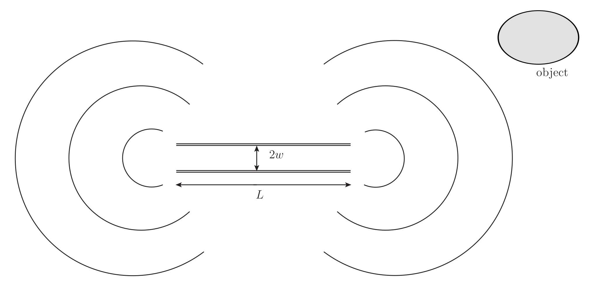We expanded quantum water dipole fields in terms of spherical harmonics and adopted a two-energy level approximation for the water dipole field in ground state ${\psi }_s$, that in the first excited states is ${\psi }_{\alpha }$ with $\alpha =0,\pm 1$ and their complex conjugates. Beginning with time evolution equations, we derived a solution for super-radiance, which is a cooperative spontaneous emission of radiation. The solution involves coherent waves from microtubules characterized by their cylindrical structures and abundantly present in all neuronal cells. The super-radiant waves propagate in a wide range by diffraction due to the small Fresnel number $\mathcal{F}\simeq {10}^{-6}$ for the structures of microtubules. The super-radiance solution offers a new method to achieve holographic memory with the interference patterns of reference waves and object waves reflected by objects involving the information of external stimuli. The transmission of electric fields $\propto -1/Z_0$, with the population difference of coherent dipoles between the first excited states and the ground state $Z_0=|{\overline{\psi }}_0{|}^2-{\left|{\overline{\psi }}_s\right|}^2$ with bar representing expectation values, is expressed in terms proportional to the squared electric fields with interference patterns in recording the information in holograms. The recorded information is reconstructed by incident reference waves whose incident angle is equal to the angle in the recording. In simulations of the time evolution of interference patterns, the wavefronts of electric fields seem to be maintained and the contrasts of electric fields are amplified. The distribution of the dipole fields has a similar form to that of electric fields in Figure 13 and Figure 14. The transmission $\propto -1/Z_0\propto 1+\frac{3}{8}{\mathcal{M}}_3^2=1+\frac{3}{8}{\eta }^2{E_3^{\prime }}^2$ with a scaled value ${\mathcal{M}}_3={\overline{\mu }}_3/(e{d}_{e}N/V)$ for the dipole moment density and proportionality constant $\eta$ contains terms dependent on the distribution of electric fields $|E_3^{\prime }{|}^2$ in recording information. Considering the fact that the wavefronts $E_3^{\prime }$ are maintained with contrasts amplified and the transmission contains terms proportional to $|E_3^{\prime }{|}^2$, the strength of the reconstructed images in recalling memory increases over the time evolution of holograms.

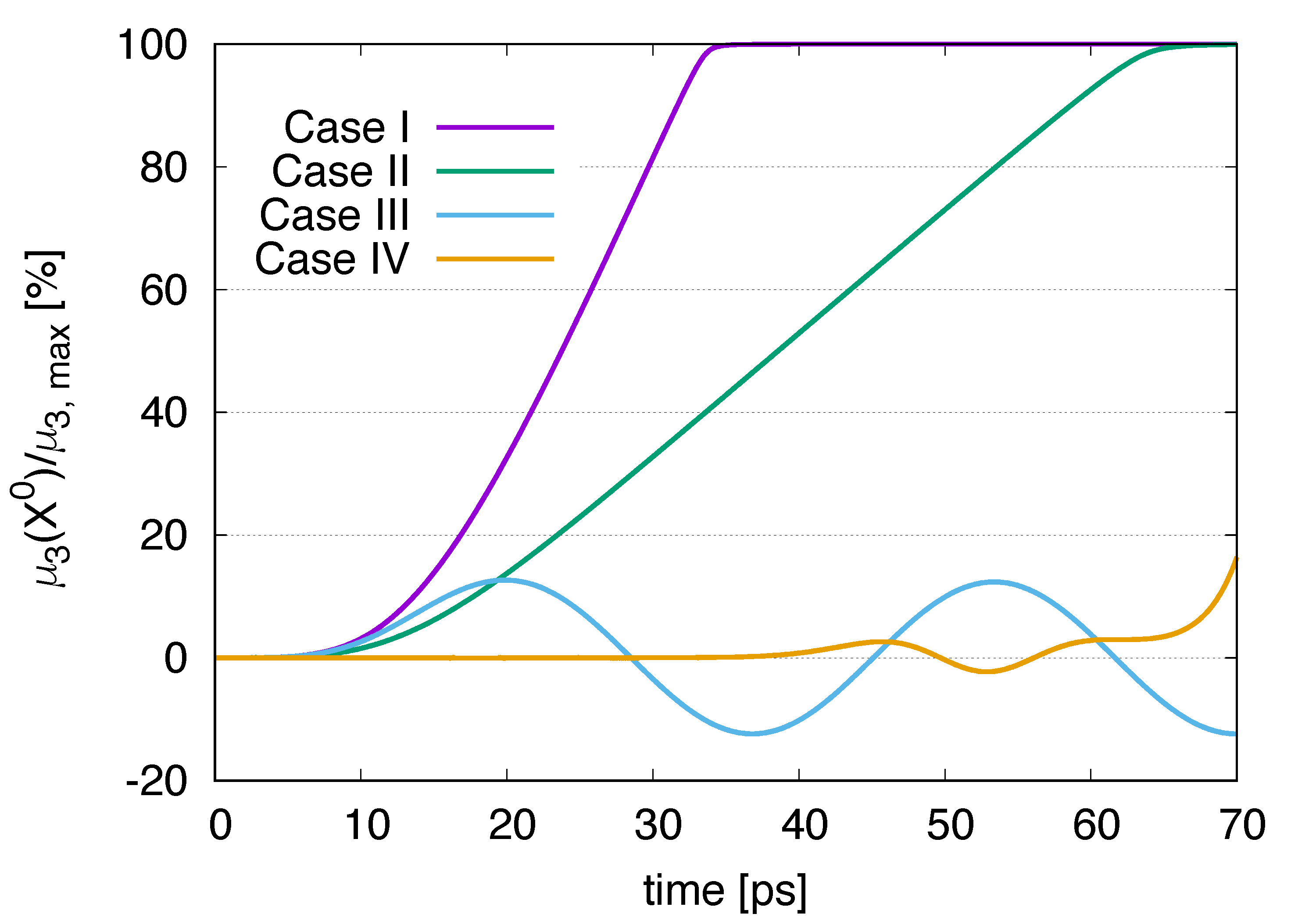
We initially began with simulations of time evolution of coherent fields in spatially homogeneous systems. We find that the breakdown of rotational symmetry emerges in time evolution with terms for quantum fluctuations derived in Appendix A. In our simulations, the positive values of the population difference of incoherent dipoles, namely the inverted population of incoherent dipoles where the population of incoherent dipoles in the first excited state is larger than that in the ground state in two-energy systems expressed by $f_2={\int }_p(F_{00}-F_{ss})/(N/V)>0$ with $F_{00,\mathrm{or},ss}$ which represent populations of incoherent dipoles for the first excited state 00 and the ground state $ss$, play a significant role in the breakdown of rotational symmetry. Dipole fields can be energy sources for coherent electric fields. We show leading-order processes of interactions in the coupling expansion in Figure 16 where Figure 16a represents processes between electric fields and incoherent dipoles, and Figure 16b represents the process of incoherent dipoles in the ground state absorbing incoherent photons and excited by the first excited states (the inverse process is also possible). 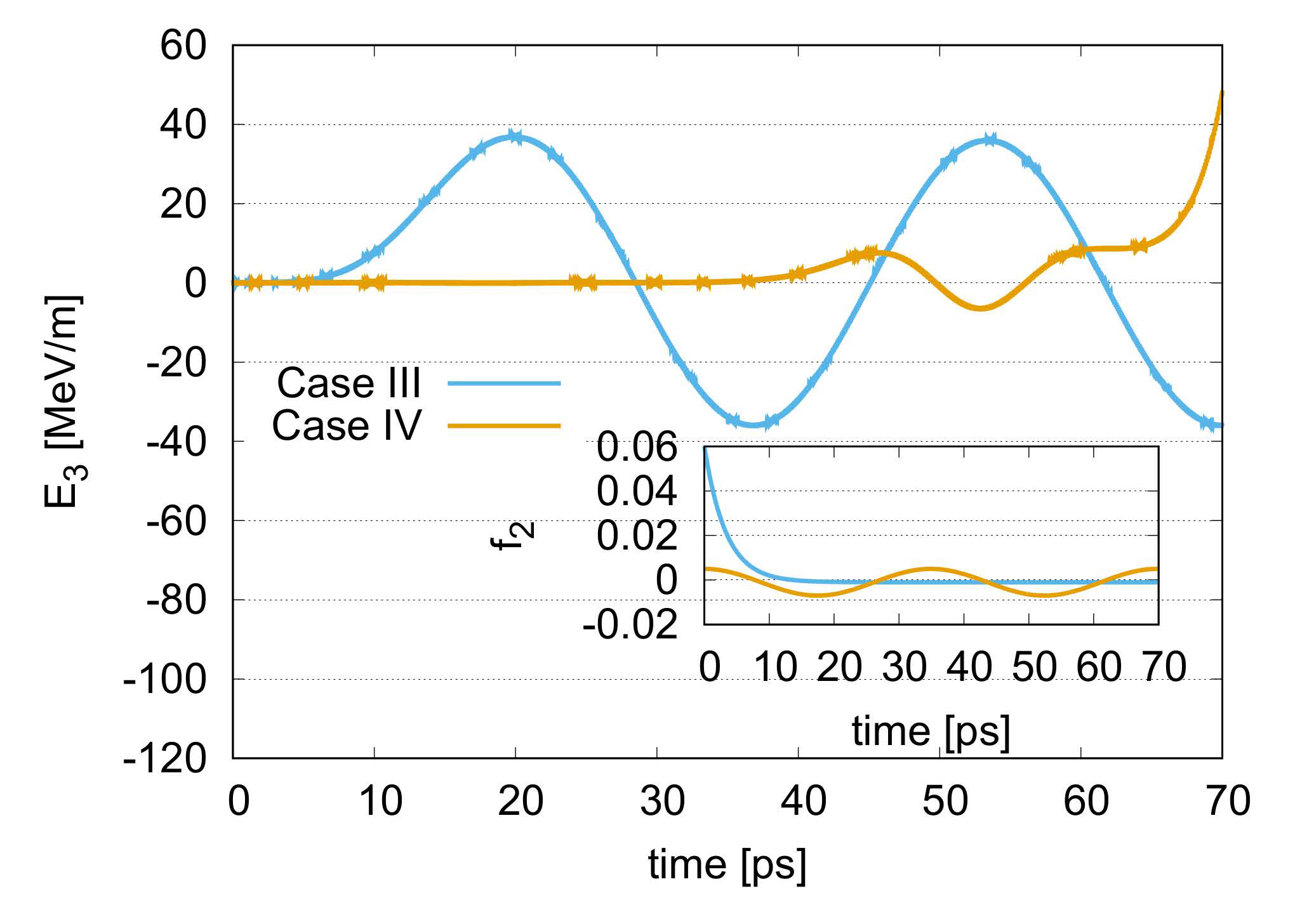By adopting open systems, we can consider the flow of incoherent photons and exciting dipoles in the ground state to the first excited states as in Figure 16b. Incoherent dipoles in the first excited states amplify electric fields in an inverted population as shown in Figure 16a. Meanwhile, electric fields oscillate in the normal population $f_2<0$. 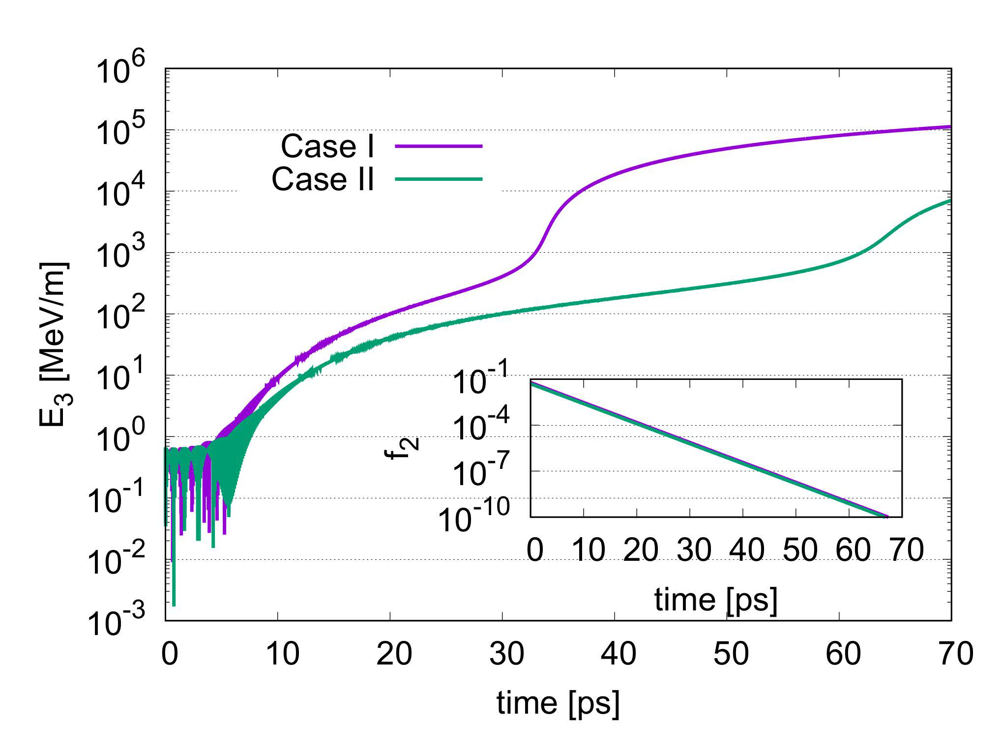The $f_2=0$ represents the threshold determining the amplification or oscillation of electric fields in spatially homogeneous systems. We can also discuss the values of electric fields in Figure 4 for which the dipole moment density ${\overline{\mu }}_3$ becomes saturated in Figure 6. Water dipoles are found to be all aligned approximately for E₃ > 1000 MeV/m in our approach based on quantum field theory (QFT). In the preceding work [49], the critical value of the external electric field inducing aligned water dipoles was determined as 800 MeV/m. We can observe that our approach provides a value of electric fields for the alignment of water dipoles similar to the value in the preceding work even if we adopt several approximations, namely an isotropic moment of inertia, a two-energy level approximation, rigid dipoles without the stretching of O–H bonds, and situations neglecting hydrogen bonding among water molecules.

Linear dependence between the logarithm of transmission $-1/Z_0$ and the logarithm of electric fields $E_3$ is observed in Figure 7. The transmission is dependent on processes of $E_3$ when $E_3$ is fluctuating at approximately zero. As $E_3$ increases exponentially, we find the relation between transmission and $E_3$ independent of processes. Even if electric fields for interference patterns are small at the initial time, they are amplified due to incoherent dipoles in the inverted population. Subsequently, transmission which is linearly dependent on amplified electric fields involving initial interference patterns is achieved in the course of time evolution. We can adopt this linear dependence for hologram memory formation.

Why is the waveform in the hologram shown in Figure 13 maintained? We can explain the reason by referring to the structure of the Klein–Gordon Equation (34). We find that the equation has the following terms

$$\begin{array}{ccc}\hfill {\Omega }^2{f}_2{E}_3+\left[{\left({\partial }^1\right)}^2+{\left({\partial }^2\right)}^2\right]E_3& =& {\Omega }^2{f}_2{E}_3-({\Theta }^2+\delta {\Theta }^2)E_3\hfill \\ & =& \left[{\Omega }^2{f}_2-({\Theta }^2+\delta {\Theta }^2)\right]E_3,\hfill \end{array}$$

(76)

with a collective mode $\Omega =\frac{13}{I}$. We assume that the population difference of incoherent dipoles $f_2={\int }_p\left(F_{00}-F_{ss}\right)/(N/V)$ is positive and sufficiently large compared with the absolute value of the curvature or spatial frequency squared of electric fields ${\Theta }^2$ emerging from the Laplacian operating on the electric fields. The $\delta {\Theta }^2$ represents the deviation of curvature from ${\Theta }^2$ in $E_3$. The larger the bracket in the above equation ${\Omega }^2{f}_2-({\Theta }^2+\delta {\Theta }^2)$ is, the more rapidly electric fields $E_3$ increase in the course of time evolution. When the deviation $\delta {\Theta }^2>0$ becomes large for the parts of interference patterns with $E_3>0$ or their absolute value of the curvature becomes large, the ${\Omega }^2{f}_2-({\Theta }^2+\delta {\Theta }^2)$ becomes smaller and the increase in parts in $E_3$ becomes moderate compared with the other parts in $E_3$. Similarly for the deviation $\delta {\Theta }^2<0$, the parts in $E_3$ increase more rapidly than the other parts. As a result, the waveform in the hologram is maintained.

In this work, we adopted a two-dimensional flat surface with periodic boundary conditions. There are various structures in morphology, that is torus, cylindrical or spherical structures with curvatures representing dendrite, cell body and axion in a brain. In these structures, we can investigate the Laplacian with derivatives in perpendicular directions to electric fields in the Klein–Gordon equation. When electric fields are in the direction perpendicular to the surfaces of cylindrical structures, the derivatives of the Laplacian is in the direction parallel to the surfaces. Then, for the zero-points of electric fields $E_r=sin\left(n\theta \right)$ with integer n and the variable of angle $\theta$, the Laplacian $\frac{1}{r^2}\frac{{\partial }^2{E}_r}{\partial {\theta }^2}$ is zero, so that electric fields in these zero-points remain zero. Except in those zero points, electric fields can be amplified in a similar way to a flat two-dimensional surface. The dipole moment density can be aligned in the same directions as electric fields in cylindrical structures. We can also discuss the various morphology of microtubules. When the diameter of microtubules becomes larger, the number of correlated water dipoles increases inside microtubules, but the amplitude of super-radiance does not change in Equation (64) since it depends on the number density of water dipoles. The critical factor is the length L of microtubules. The larger the length is, the smaller ${\tau }_R$ is, so that the amplitude of super-radiance will increase since that is proportional to the length. The length of microtubules affects the initial electric fields in the interference patterns of holography. In addition, the number of microtubules becomes larger, the diverse angles and sources of super-radiant emission will be achieved, and the capacity of hologram memory can increase.

We consider memory printing and information processing induced by external stimuli in QBD and holography. The candidate of initial external objects might be phosphorylated tubulins [1] and ionic bio-plasma around microtubules, for example, in V1 for visual information. External objects in V1 are irradiated by super-radiant waves. Then, the interference patterns of reference and object waves are produced as holographic patterns. Once these optical patterns of holography are produced, they propagate in a brain with the other super-radiant waves from neurons in a higher visual cortex with parallel information processing. The strength and angle will be determined by the distances and geometry in the propagation of the visual cortex, which is the strength and angle of super-radiance that depend on the distance of propagation and the direction of information processing in the cortex.

In conventional neuroscience, we consider long-term potentiation (LTP) as a result of neurotransmitter-receptors as the mechanism of long-term memory. Our approach can connect the LTP and holographic approach with super-radiant waves. We shall consider the firing of a single neuron and subsequent super-radiant emissions. There can be various angles of super-radiant emissions as reference waves inducing the reconstruction of multiple holographic images. In considering the firing of two neurons interconnected by LTP with synchrony, the common reconstructed image can emerge in both printing and recalling, and then the amplitude of that image is twice that of the other images. Similarly, due to the firing of N multiple neurons with synchrony and subsequent super-radiant emissions, the amplitude of the common image is N times larger than that of the other images regarded as noises. As a result of LTP and subsequent super-radiant emission, the synchrony can induce the common holographic image in printing and recalling whose amplitude might be proportional to the number of neurons with synchrony.

We adopt the QFT approach involving the field variables of space–time coordinates. The QFT approach can be regarded as the generalization of multi-oscillator systems. In [50,51,52,53], the sets of oscillators with a mutual relationship with temporal synchrony for binding and robustness in conscious perception against inherent noise are reported. Similarly, we can consider the mass-spring system of oscillators with an infinite number of point-masses and spring among (neighboring) them in the continuum limit. This physical system will be represented by field variables defined in each space–time in QFT including strings, cloths, or boxes. The QFT with an infinite number of degrees of freedom can provide the Bose–Einstein condensation where massless Nambu–Goldstone bosons are condensed in the zero-energy state resulting in the binding of quantum degrees of freedom in the physical system where they behave as a single entity. The QFT generalized from oscillators can provide the binding of quantum degrees of freedom and synchrony in the physical system. The QFT might provide an answer to the binding problem in neuroscience.

Our approach can provide relations with a split brain study suggested in [54,55]. Among the consequences of cutting the corpus callosum, the breakdown of functional integration between the left and right hemispheres is reported. We assume that the brain is a mixed system of classical neurons and quantum degrees of freedom. Connections among neurons play a role in synchrony. In the split brain, although memory is not lost in each hemisphere due to the diffused non-local nature of memory, the synchrony among neurons is lost. Due to the loss of connections, the simultaneous neuron firing and synchrony of subsequent super-radiant emissions will disappear.

We can adopt parallel information processing in the hologram memory of QBD, where the processing is optically achieved in each point of the hologram through propagation in space. The optical information of a hologram memory might be transferred with the filtering of the hologram or processing in propagation through a hierarchy in the neocortex. (The digital–analog conversion with filtering is proposed in [56].) Hologram memory might propagate in the hierarchy and can be stored in an invariant form of memory. In storing information in the hologram, we do not necessarily adopt sine functions for transmission. We can also adopt step-function-like storage, where coherent domains with dipoles are all aligned and incoherent domains with dipoles whose directions are random are distributed as spatially inhomogeneous patterns after optical information processing. The difference between sine functions and step functions is one of efficiency. This denotes the percentage of incident reference beam used to reconstruct the object image. The holograms for long-term memory might be stored as step functions with coherent domains and incoherent domains and be diffused in a whole brain to achieve the equipotentiality and the mass action. When we consider step-function-like storage, we can then adopt the vacua emerging in the breakdown of rotational symmetry. The vacua are long-range correlations maintained by massless Nambu–Goldstone bosons, indicating robustness against disturbance. We find several stable examples of the breakdown of symmetry in our daily life. For example, magnets are maintained by magnons in the breakdown of symmetry and crystals are maintained by phonons in room temperature. We just simply propose to adopt the macroscopic order emerging in the breakdown of symmetry in quantum field theory (QFT) in QBD and holography. The QFT, the fundamental theory of the nature describes both macroscopic matter (including macroscopic order in the breakdown of symmetry) in classical mechanics and microscopic degrees of freedom in quantum mechanics. The QFT approach is different from other quantum mechanical approaches, such as Penrose–Hameroff theory [57]. The quantum mechanics cannot be applied to macroscopic matter. The robustness against damage in a brain is achieved in hologram memory. The whole image can be recreated from undamaged parts in hologram memory even if parts of the hologram are damaged. We can represent sequential characters of hologram memory. When patterns of incident super-radiant emission are sequential, this may be related to neuron firing and subsequent super-radiant beams in sequential properties—we recall memory as sequential patterns. We can also achieve the auto-associative character of memory in a brain by adopting hologram memory in QBD, where the entire memory is recreated from fragments of memory. When two object images are recorded on the same hologram and the reflected light by one of the object images extends to the hologram, the other object image is recreated by the light.

6. Conclusions and Perspectives

We proposed the integration of quantum brain dynamics (QBD) and holography. Based on the Lagrangian density of QBD, we derived the time evolution equations for coherent dipole fields and coherent electric fields. We adopted a solution of super-radiance to achieve interference patterns for hologram memory. We discovered that the breakdown of rotational symmetry occurs in an inverted population of incoherent dipoles in spatially homogeneous systems. We investigated how interference patterns in holographic memory evolve over time with the existence of the flow of dipole fields in the first excited state (quantum fluctuations) excited by incoherent photons. Ordered patterns in a hologram were amplified for memory printing in the course of time evolution in the inverted population of the incoherent dipoles. Holography in QBD can describe several properties of memory in a brain, which are different from computer memory. The integration of QBD and holography may provide a promising approach to investigate the fundamental and applied aspects of the human brain and the mechanism of memory creation.

References

1. Craddock, T.J.A.; Tuszynski, J.A.; Hameroff, S. Cytoskeletal Signaling: Is Memory Encoded in Microtubule Lattices by CaMKII Phosphorylation? PLoS Comput. Biol. 2012, 8, e1002421. [Google Scholar] [CrossRef] [PubMed] [Green Version]
2. Hawkins, J.; Blakeslee, S. On Intelligence; Macmillan: Stuttgart, Germany, 2004. [Google Scholar]
3. Okada, K.; Rong, F.; Venezia, J.; Matchin, W.; Hsieh, I.H.; Saberi, K.; Serences, J.T.; Hickok, G. Hierarchical organization of human auditory cortex: Evidence from acoustic invariance in the response to intelligible speech. Cereb. Cortex 2010, 20, 2486–2495. [Google Scholar] [CrossRef] [PubMed]
4. Evans, S.; Davis, M.H. Hierarchical organization of auditory and motor representations in speech perception: Evidence from searchlight similarity analysis. Cereb. Cortex 2015, 25, 4772–4788. [Google Scholar] [CrossRef] [PubMed]
5. Rolls, E.T. Neurophysiological mechanisms underlying face processing within and beyond the temporal cortical visual areas. Philos. Trans. R. Soc. Lond. Ser. B Biol. Sci. 1992, 335, 11–21. [Google Scholar]
6. Wallis, G.; Rolls, E.; Foldiak, P. Learning invariant responses to the natural transformations of objects. In Proceedings of the 1993 International Conference on Neural Networks, Nagoya, Japan, 25–29 October 1993; Volume 2, pp. 1087–1090. [Google Scholar] [CrossRef]
7. Rolls, E.T. Brain mechanisms for invariant visual recognition and learning. Behav. Process. 1994, 33, 113–138. [Google Scholar] [CrossRef]
8. Bartlett, F.; John, E. Equipotentiality quantified: The anatomical distribution of the engram. Science 1973, 181, 764–767. [Google Scholar] [CrossRef] [PubMed]
9. Lashley, K.S. Brain Mechanisms and Intelligence: A Quantitative Study of Injuries to the Brain; University of Chicago Press: Chicago, IL, USA, 1929. [Google Scholar]
10. Jibu, M.; Yasue, K. Quantum Brain Dynamics and Consciousness; John Benjamins: Amsterdam, The Netherlands, 1995. [Google Scholar]
11. Vitiello, G. My Double Unveiled: The Dissipative Quantum Model of Brain; John Benjamins Publishing: Amsterdam, The Netherlands, 2001; Volume 32. [Google Scholar]
12. Ricciardi, L.M.; Umezawa, H. Brain and physics of many-body problems. Kybernetik 1967, 4, 44–48. [Google Scholar] [CrossRef] [PubMed]
13. Stuart, C.; Takahashi, Y.; Umezawa, H. On the stability and non-local properties of memory. J. Theor. Biol. 1978, 71, 605–618. [Google Scholar] [CrossRef]
14. Stuart, C.; Takahashi, Y.; Umezawa, H. Mixed-system brain dynamics: Neural memory as a macroscopic ordered state. Found. Phys. 1979, 9, 301–327. [Google Scholar] [CrossRef]
15. Fröhlich, H. Bose condensation of strongly excited longitudinal electric modes. Phys. Lett. A 1968, 26, 402–403. [Google Scholar] [CrossRef]
16. Fröhlich, H. Long-range coherence and energy storage in biological systems. Int. J. Quantum Chem. 1968, 2, 641–649. [Google Scholar] [CrossRef]
17. Davydov, A.; Kislukha, N. Solitons in One-Dimensional Molecular Chains. Phys. Status Solidi B 1976, 75, 735–742. [Google Scholar] [CrossRef]
18. Tuszyński, J.; Paul, R.; Chatterjee, R.; Sreenivasan, S. Relationship between Fröhlich and Davydov models of biological order. Phys. Rev. A 1984, 30, 2666. [Google Scholar] [CrossRef]
19. Del Giudice, E.; Doglia, S.; Milani, M.; Vitiello, G. Spontaneous symmetry breakdown and boson condensation in biology. Phys. Lett. A 1983, 95, 508–510. [Google Scholar] [CrossRef]
20. Del Giudice, E.; Doglia, S.; Milani, M.; Vitiello, G. A quantum field theoretical approach to the collective behaviour of biological systems. Nucl. Phys. B 1985, 251, 375–400. [Google Scholar] [CrossRef]
21. Del Giudice, E.; Preparata, G.; Vitiello, G. Water as a free electric dipole laser. Phys. Rev. Lett. 1988, 61, 1085. [Google Scholar] [CrossRef]
22. Del Giudice, E.; Smith, C.; Vitiello, G. Magnetic Flux Quantization and Josephson Systems. Phys. Scr. 1989, 40, 786–791. [Google Scholar] [CrossRef]
23. Jibu, M.; Yasue, K. A physical picture of Umezawa’s quantum brain dynamics. Cybern. Syst. Res. 1992, 92, 797–804. [Google Scholar]
24. Jibu, M.; Yasue, K. Intracellular quantum signal transfer in Umezawa’s quantum brain dynamics. Cybern. Syst. 1993, 24, 1–7. [Google Scholar] [CrossRef]
25. Jibu, M.; Hagan, S.; Hameroff, S.R.; Pribram, K.H.; Yasue, K. Quantum optical coherence in cytoskeletal microtubules: Implications for brain function. Biosystems 1994, 32, 195–209. [Google Scholar] [CrossRef]
26. Jibu, M.; Yasue, K. What is mind?—Quantum field theory of evanescent photons in brain as quantum theory of consciousness. Informatica 1997, 21, 471–490. [Google Scholar]
27. Jibu, M.; Yasue, K. Magic without magic: Meaning of quantum brain dynamics. J. Mind Behav. 1997, 18, 205–227. [Google Scholar]
28. Vitiello, G. Dissipation and memory capacity in the quantum brain model. Int. J. Mod. Phys. B 1995, 9, 973–989. [Google Scholar] [CrossRef]
29. Pribram, K.H. Languages of the Brain: Experimental Paradoxes and Principles in Neuropsychology; Prentice-Hall: Hoboken, NJ, USA, 1971. [Google Scholar]
30. Pribram, K.H.; Yasue, K.; Jibu, M. Brain and Perception: Holonomy and Structure in Figural Processing; Psychology Press: London, UK, 1991. [Google Scholar]
31. Gabor, D. A new microscopic principle. Nature 1948, 161, 777–778. [Google Scholar] [CrossRef]
32. Hariharan, P. Optical Holography: Principles, Techniques and Applications; Cambridge University Press: Cambridge, UK, 1996. [Google Scholar]
33. Nishiyama, A.; Tanaka, S.; Tuszynski, J.A. Non-equilibrium Quantum Brain Dynamics II: Formulation in 3+1 dimensions. Phys. A: Stat. Mech. Its Appl. 2021, 567, 125706. [Google Scholar] [CrossRef]
34. Cornwall, J.M.; Jackiw, R.; Tomboulis, E. Effective action for composite operators. Phys. Rev. D 1974, 10, 2428. [Google Scholar] [CrossRef]
35. Calzetta, E.; Hu, B.L. Nonequilibrium quantum fields: Closed-time-path effective action, Wigner function, and Boltzmann equation. Phys. Rev. D 1988, 37, 2878. [Google Scholar] [CrossRef]
36. Berges, J. Introduction to nonequilibrium quantum field theory. In AIP Conference Proceedings; American Institute of Physics: College Park, MD, USA, 2004; Volume 739, pp. 3–62. [Google Scholar]
37. Baym, G.; Kadanoff, L.P. Conservation laws and correlation functions. Phys. Rev. 1961, 124, 287. [Google Scholar] [CrossRef]
38. Kadanoff, L.P.; Baym, G. Quantum Statistical Mechanics: Green’s Function Methods in Equilibrium Problems; WA Benjamin: Los Angeles, CA, USA, 1962. [Google Scholar]
39. Baym, G. Self-consistent approximations in many-body systems. Phys. Rev. 1962, 127, 1391. [Google Scholar] [CrossRef]
40. Kluberg-Stern, H.; Zuber, J. Renormalization of non-Abelian gauge theories in a background-field gauge. I. Green’s functions. Phys. Rev. D 1975, 12, 482. [Google Scholar] [CrossRef]
41. Abbott, L.F. The background field method beyond one loop. Nucl. Phys. B 1981, 185, 189–203. [Google Scholar] [CrossRef] [Green Version]
42. Abbott, L.F. Introduction to the background field method. Acta Phys. Pol. B 1981, 13, 33–50. [Google Scholar]
43. Wang, Q.; Redlich, K.; Stöcker, H.; Greiner, W. From the Dyson–Schwinger to the transport equation in the background field gauge of QCD. Nucl. Phys. A 2003, 714, 293–334. [Google Scholar] [CrossRef] [Green Version]
44. Schwinger, J. Brownian motion of a quantum oscillator. J. Math. Phys. 1961, 2, 407–432. [Google Scholar] [CrossRef]
45. Keldysh, L.V. Diagram technique for nonequilibrium processes. Sov. Phys. JETP 1965, 20, 1018–1026. [Google Scholar]
46. Bonifacio, R.; Preparata, G. Coherent spontaneous emission. Phys. Rev. A 1970, 2, 336. [Google Scholar] [CrossRef]
47. Benedict, M.G. Super-Radiance: Multiatomic Coherent Emission; CRC Press: Boca Raton, FL, USA, 1996. [Google Scholar]
48. Gross, M.; Haroche, S. Superradiance: An essay on the theory of collective spontaneous emission. Phys. Rep. 1982, 93, 301–396. [Google Scholar] [CrossRef]
49. Tokman, M.; Lee, J.H.; Levine, Z.A.; Ho, M.C.; Colvin, M.E.; Vernier, P.T. Electric Field-Driven Water Dipoles: Nanoscale Architecture of Electroporation. PLoS ONE 2013, 8, e61111. [Google Scholar] [CrossRef] [Green Version]
50. Kraikivski, P. Building systems capable of consciousness. Mind Matter 2017, 15, 185–195. [Google Scholar]
51. Kraikivski, P. Systems of oscillators designed for a specific conscious percept. New Math. Nat. Comput. 2020, 16, 73–88. [Google Scholar] [CrossRef] [Green Version]
52. Kraikivski, P. Implications of Noise on Neural Correlates of Consciousness: A Computational Analysis of Stochastic Systems of Mutually Connected Processes. Entropy 2021, 23, 583. [Google Scholar] [CrossRef]
53. Kraikivski, P. A Dynamic Mechanistic Model of Perceptual Binding. Mathematics 2022, 10, 1135. [Google Scholar] [CrossRef]
54. Bogen, J.E.; Fisher, E.; Vogel, P. Cerebral commissurotomy: A second case report. JAMA 1965, 194, 1328–1329. [Google Scholar] [CrossRef]
55. De Haan, E.H.; Corballis, P.M.; Hillyard, S.A.; Marzi, C.A.; Seth, A.; Lamme, V.A.; Volz, L.; Fabri, M.; Schechter, E.; Bayne, T.; et al. Split-brain: What we know now and why this is important for understanding consciousness. Neuropsychol. Rev. 2020, 30, 224–233. [Google Scholar] [CrossRef]
56. Nakajima, M.; Morikawa, T.; Sakurai, K. Automatic character reading using a holographic data processing technique. Appl. Opt. 1972, 11, 362–371. [Google Scholar] [CrossRef]
57. Penrose, R. The Emperor’s New Mind: Concerning Computers, Minds, and the Laws of Physics; Oxford University Press: Oxford, UK, 1989. [Google Scholar]
Figure 1. The flowchart of derivation.
Dynamics 02 00010 g001
Figure 2. Super-radiant emission from a microtubule.
Dynamics 02 00010 g002
Figure 3. Interference of reference and object waves.
Dynamics 02 00010 g003
Figure 4. Time-evolution of the electric field E 3 with population difference f 2 in Cases I and II.
Dynamics 02 00010 g004
Figure 5. Time-evolution of the electric field E 3 with population difference f 2 in Cases III and IV.
Dynamics 02 00010 g005
Figure 6. Time-evolution of dipole moment density μ ¯ 3 divided by its maximum value μ 3 , max .
Dynamics 02 00010 g006
Figure 7. Time-evolution of population difference of coherent dipole fields Z = Z 0 / ( N / V ) .
Dynamics 02 00010 g007
Figure 8. Population difference of coherent dipole fields Z for the electric field E 3 in Cases I, II, III, and IV.
Dynamics 02 00010 g008
Figure 9. Time-evolution of electric field E 3 ( x 0 , x 1 = 32 a s , x 2 = 0 ) .
Dynamics 02 00010 g009
Figure 10. Distribution of the electric field E 3 at x 0 = 50 ps , x 0 = 300 ps and x 0 = 450 ps .
Dynamics 02 00010 g010
Figure 11. Distribution of the dipole moment density μ ¯ 3 divided by its maximum value μ ¯ 3 , max = 2 3 e d e N / V at x 0 = 50 ps , x 0 = 300 ps and x 0 = 450 ps .
Dynamics 02 00010 g011
Figure 12. Distribution of the population difference of coherent dipoles Z 0 / ( N / V ) at x 0 = 50 ps , x 0 = 300 ps and x 0 = 450 ps .
Dynamics 02 00010 g012
Figure 13. Distribution of electric fields E 3 at (a) x 0 = 0.0 ps ; (b) x 0 = 5.0 ps ; (c) x 0 = 6.0 ps ; and (d) x 0 = 7.0 ps .
Dynamics 02 00010 g013
Figure 14. Distribution of the dipole moment density μ ¯ 3 divided by the maximum value μ 3 = 2 3 e d e N / V at x 0 = 7.0 ps .
Dynamics 02 00010 g014
Figure 15. Distribution of population difference Z 0 / ( N / V ) at x 0 = 7.0 ps .
Dynamics 02 00010 g015
Figure 16. Leading-order processes of interactions in the coupling expansion of e d e . (a) Interaction between electric fields and incoherent dipoles in the ground states and the first excited states; and (b) Interaction between incoherent photons and incoherent dipoles.
Dynamics 02 00010 g016