Orbital Dynamics in the Restricted Three Body Problem: Overview of Recent Analytical Advances Obtained by Separating Rapid and Slow Subsystems in Non-Planar Configurations

Abstract

Analytical solutions to a variety of simplified versions of the restricted three-body problem in celestial mechanics possess long running history that encompasses several centuries. Most of the successes were limited either to the planar configuration of the three bodies, to the motion around the Lagrange points, or to the Kozai–Lidov effect. We review some analytical advances obtained by separating rapid and slow subsystems as presented in recently published papers concerning the non-planar motion of the three bodies unrelated to the Lagrange points and to the Kozai–Lidov effect. Most (but not all) of the discussed advances correspond to the bound motion in the considered celestial systems.

1. Introduction

It is well-known that the classical three-body problem, which has the history of several centuries, does not have a general analytical solution. Analytical advances were made for the restricted three-body problem, i.e., for the situation where the third body has a negligible mass.

Most of the successes in the restricted three-body problem were limited either to the planar geometry, to the motion around the Lagrange points, or to the Kozai–Lidov effect. The interested reader can refer to books, e.g., by Butikov [1], Brouwer and Clemence [2], Smart [3], Fitzpatrick [4], Sterne [5], Koon et al. [6], Beutler [7], Celetti [8], and Valtonen and Karttunen [9] (and the references in these books); and reviews by Naoz [10] and Musielac and Quarles [11] (and the references in these reviews); as well as recent papers by Napier et al. [12], Vashkov’yak [13], Wang et al. [14], Quarles et al. [15], Gao and Wang [16,17,18], Mittal et al. [19], Abouelmagd et al. [20], Li and Liao [21], Sindik et al. [22], Vinson and Chiang [23], Naoz et al. [24], Orlov et al. [25], Lei and Xu [26], and the references in these papers.

In the last several years, there have been published papers presenting analytical results, obtained by separating rapid and slow subsystems on the non-planar motion of the three bodies unrelated to the Lagrange points and to the Kozai–Lidov effect. These advances in the restricted three body problem concern both the bound motion and the unbound motion in the considered celestial systems. The review is structured as follows.

In Section 2, we review the analytical results from a paper by Oks [27] on the non-planar motion of a planet around a binary star. In Section 3 and Section 4, we overview the analytical results from a paper by Kryukov and Oks [28] on relativistic corrections to the results from Section 2 and on the non-planar motion of a moon in a star-planet system. In Section 5, we review the analytical results from paper by Oks [29] on the non-planar motion of a circumbinary planet. These results represent an extension of the corresponding analytical results obtained by Farago and Laskar [30] and the results previously obtained by Schneider [31]. In Section 6, we overview the analytical results from a paper by Oks [32] on the motion of an interstellar interloper in the vicinity of the circular binary star. In Section 7, we review the analytical results from paper by Oks [33] on an alternative method for detecting and measuring parameters of a compact dark matter object that constitutes a component of a binary system—the results involving the non-planar motion of a planet in this system. In Section 8, we overview analytical results from a paper by Oks [34] on the circular Sitnikov problem in a more general setup and compare them with the corresponding analytical results obtained by Belbruno et al. [35] only for the special case of the circular Sitnikov problem. In Section 9, we provide concluding remarks. In Appendix A, we relax the assumption of the circular orbits of the stars in the binary—the assumption used in Section 5—and present analytical results on the effect of a low-eccentricity of the orbits of the stars on the motion of the circumbinary planet.

2. Non-Planar Motion of a Planet around a Binary Star: Nonrelativistic Motion

In the papers by Oks [27,36], the author started by analyzing a model system consisting of two fixed stars of masses μ and μ′ that are separated by a distance R and a planet of a unit mass revolving in a circular orbit in the plane perpendicular to the interstellar axis (the circle being centered at the interstellar axis). The analytical treatment was performed in the cylindrical coordinates (z, ρ, and φ) with the z-axis directed from the mass μ (located at the origin) to the mass μ′ (located at z = R). Due to the cylindrical symmetry, the z-motions and ρ-motions were separated from the φ-motion.

The following notations were introduced:

w ≡ z/R, v ≡ ρ/R, b ≡ μ′/μ, Z = Gμ, m ≡ M/(ZR)^1/2,

(1)

where G is the gravitational constant and M is the projection of the planet angular momentum on the interstellar axis. Here w, v, and m are the scaled and dimensionless counterparts of the coordinate z, coordinate ρ, and the projection M of the planet angular momentum, respectively; b is the ratio of the stellar masses.

In the scaled notations, the effective potential energy can be represented in the following form.

U_eff ≡ (Z/R) u_eff(w, v, m, b), u_eff(w, v, m, b) = m²/(2v²) − (w² + v²)^−1/2 − b[(1 − w)² + v²]^−1/2

(2)

After the derivatives of the effect potential energy with respect to w and with respect to v were equated to zero, it was found that the locus of the equilibrium points in the plane (w, v) is the line v₀ (w, b) defined by the following equation.

v₀(w, b) = {[w^2/3(1 − w)^4/3 − b^2/3w²]/[b^2/3 − w^2/3/(1 − w)^2/3]}^1/2.

(3)

As an example, Figure 1 shows the dependence v₀(w) for b = 2 (we note that the ratio of masses b = μ′/μ in the observed binaries ranges from ~1 to ~10²). It is observed that there are two ranges of the scaled coordinate w where the equilibria exist. For an arbitrary b > 1, these two ranges are as follows: 0 ≤ w ≤ 1/(1 + b^1/2) and b/(1 + b) < w ≤ 1.

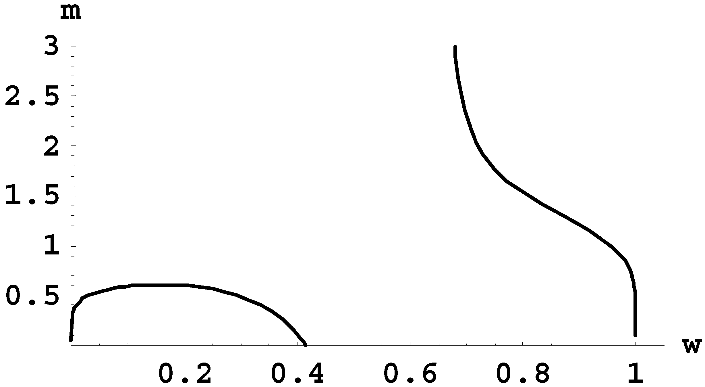
The dependence of the equilibrium value of the scaled projection of the angular momentum on the scaled coordinate w turned out to be the following.

m₀(w, b) = v₀²(w, b)/{(1 − w)^1/2[w² + v₀²(w, b)]^3/4}

(4)

Figure 2 illustrates this dependence for b = 2.

A scaled total energy e was defined as follows:

E ≡ (Z/R) e(w, b),

(5)

where e(w, b) turned out to be the following.

e(w, b) = − [w(1 − w) + v₀²(w, b)/2]/{(1 − w)[w² + v₀²(w, b)]^3/2}

(6)

From this point on, the angular momentum projection was considered as a parameter possessing some positive value. The interstellar distance R and the coordinate w, as well as the parameters b and M, are interrelated by the following formula.

R(w, b, M) = M²/[Z m₀²(w, b)]

(7)

The substitution of R(w, b, M) from Equation (7) in Equation (5) results in the following expression for the energy E.

E(w, b, M) = (Z/M)² m₀²(w, b) e(w, b)

(8)

For any b > 0 and M ≥ 0, the combination of Equations (7) and (8) provides parametric dependence (via the parameter w) of the energy E on the interstellar distance R. Due to the analogy with the corresponding problem from molecular physics, this dependence is named “classical energy terms”. We remind the reader that in molecular physics, quantum energy terms (i.e., the dependence of the energy on the internuclear distance R) show, in particular, how the frequency of radiative transitions ω(R) = ΔE(R)/ħ, where ΔE(R) is the difference of two energy terms, depends on R.

As an example, Figure 3 presents the scaled energy ε = (M/Z)²E as the function of the scaled interstellar distance r = (Z/M²)R for the ratio of the stellar masses b = 2. Figure 3 shows the following: (1) There exist three classical energy terms (for any fixed positive value of the angular momentum projection M); (2) two of the classical energy terms undergo a “V-shape” crossing (V being rotated clockwise by 90 degrees). At the V-shape crossing, just as it would be at the usual X-shape crossing of the terms, the system can switch from one energy term to another.

At this point it might be useful to clarify the following. The energy E and its scaled counterpart ε are related as E = (Z/M)²ε. Kryukov and Oks [28] clarified the following: “The projection M of the angular momentum on the interstellar axis is a continuous variable. The energy E depends on both ε and M. Therefore, while the scaled quantity ε takes a discrete set of values, the energy E takes a continuous set of values (as it should be in classical physics)”.

Next, Oks [27] considered small deviations from equilibrium values (w_i, v_0i, m_0i) for some fixed ratio b of the stellar masses.

δw ≡ w − w_i, δv ≡ v − v_0i.

(9)

After some calculations, it was found that under the following condition:

v₀(w, b) ≥ {w(1 − w) − 1/2 + [9w²(1 − w)² − w(1 − w) + 1/4]^1/2}^1/2 ≡ v_crit(w),

(10)

the effective potential energy has a two-dimensional minimum at the equilibrium values of w and v; this ensures that the equilibrium is stable. Furthermore, for this stable motion, the planetary trajectory is a helix on the surface of a conical fulcrum for which its axis coincides with the interstellar axis: the conic-helical state.

Next, it was necessary to take into account the effect of the stars’ rotation when proceeding to the real system. For this purpose, Oks [27] employed the analytical method using the separation of rapid and slow subsystems (concerning the general formalism of this method and a number of its applications, refer to, e.g., the book by Oks [37].

In the system under the consideration, for a sufficiently small w, the rapid subsystem was the planetary motion while the slow subsystem was the stars’ rotation. The ratio of the primary frequency of the planetary motion to the Kepler frequency of the stars rotation was the following.

k = 1/{(1 + b)^1/2(1 − w)^1/2 [w² + v₀(w, b)²]^3/4}.

(11)

As an example, Figure 4 shows this ratio versus w for the ratio of the stellar masses b = 10. It is observed that this ratio reaches very large values if the projection of the planetary orbit on the interstellar axis is relatively close to the star of the smaller mass (w << 1).

It turned out that the stars’ rotation only results in relatively small oscillations of the scaled radius of the planetary orbit v and of the scaled projection w of the planetary orbit on the interstellar axis as long as the ratio of the stars’ masses b is greater or of the order of 10 and the averaged plane of the planetary orbit is much closer to the lighter of the two stars (w << 1). This is illustrated by Figure 5 and Figure 6, which is adopted from the paper by Kryukov and Oks [28]. (Kryukov and Oks [28] also corrected some misprints from Oks paper [27]. Unfortunately, this fact has been missed by Egan [38], whose paper was almost entirely devoted to correcting the same misprints from Oks [27] paper. Egan [38] also missed the simulations performed by Kryukov and Oks [28]. This renders Egan paper [38] superfluous in both its analytical and simulative parts).

Thus, for sufficiently small w and sufficiently large b, the conic-helical orbit of the planet would remain stable for a very long period of time despite the stars’ rotation. This is a novel analytical result on the non-planar relatively stable configuration with respect to the restricted three-body problem.

We note that Naoz [10] and Naoz et al. [24] analytically considered the situation where the planet (the lowest mass body) orbits one of the stars in the binary (star 1), while the other star (star 2) is much further away compared to the average separation between the planet and star 1. While the results from these two publications are useful, their authors missed the conic-helical planetary orbits discussed in the present section of this review.

3. Non-Planar Motion of a Planet around a Binary Star: Relativistic Corrections

Kryukov and Oks [28] studied a possible role of relativistic effects in the non-planar restricted three-body problem described in Section 2. They found that the amplitudes of small oscillations of the scaled axial w and radial v coordinates about their equilibrium values (the oscillations caused by the stars rotation) in the relativistic case are the same as in the non-relativistic case. What turned out to be different in the relativistic case compared to the non-relativistic case was the ratio k of the primary frequency of the planetary motion about the interstellar axis to the frequency of the stars’ rotation:

$$\mathrm{k}=\frac{{{(\mathrm{b}}^{2/3}{\mathsf{\gamma }}^2-1)}^{3/4}{{(\mathsf{\gamma }}^3+1)}^{5/4}}{\sqrt{1+\mathrm{b}}{\mathsf{\gamma }}^{3/2}{{(\mathsf{\gamma }}^3-1)}^{3/4}}\sqrt{1-\frac{\mathsf{\mu }\mathrm{s}}{\mathrm{R}}\frac{{(\mathsf{\gamma }}^4-{\mathrm{b}}^{2/3})\sqrt{{(\mathrm{b}}^{2/3}{\mathsf{\gamma }}^2-{1\left)\right(\mathsf{\gamma }}^3+1)}}{{\mathsf{\gamma }(\mathsf{\gamma }}^3-{1)}^{3/2}}}$$

(12)

where the quantity s = GM_Sun/c² is equal to one half of the Schwarzschild radius of the Sun (approximately 147,700 cm) and M_Sun is the Sun’s mass. The parameter γ represents the equilibrium value of the scaled projection of the planetary orbit on the interstellar axis in the following manner.

$$\mathsf{\gamma }=(\frac{1}{\mathrm{w}}-1{)}^{1/3}$$

(13)

The combination of Equation (12) for k(w, b), employing the notation γ(w) from Equation (13) for brevity, and Equation (3) for the equilibrium value of the scaled radius of the orbit v(w, b) constitutes the parametric dependence of k on v for any fixed ratio b of the stellar masses.

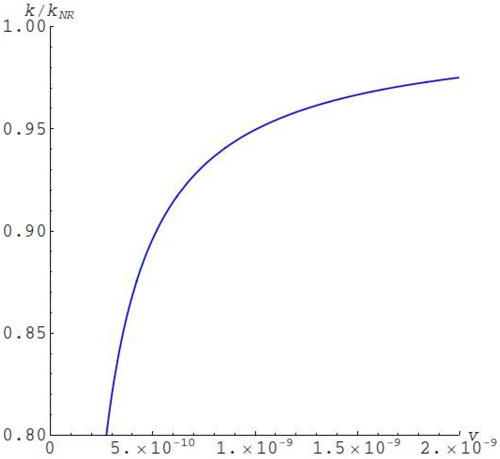
Figure 7 presents the ratio of the quantity k to its non-relativistic counterpart k_NR versus the scaled radius of the orbit v for the interstellar distance R = 100 a.u. (wide binary system) and the stars’ masses μ = 1 and μ′ = 100 (in the units of the Sun mass). One can observe that the relativistic effects become important for v~10^–9 or smaller. (Figure 7, Figure 8 and Figure 9 are adopted from the paper by Kryukov and Oks [28]).

For R = 100 a.u., the values of V = (1 ÷ 2) × 10⁻⁹ correspond to the values of the radius of the planetary orbit ρ = (15 ÷ 30) km. From the obvious requirement for the radius of the planet to be smaller than ρ, it follows that in this situation that it should be a planetoid.

Figure 8 presents the dependence k(v) for the same example as in Figure 7. It shows that, for the range of v < 2 × 10⁻⁹, the ratio of the frequencies exceeds 10¹² and, thus, such system would be stable for a very long period of time.

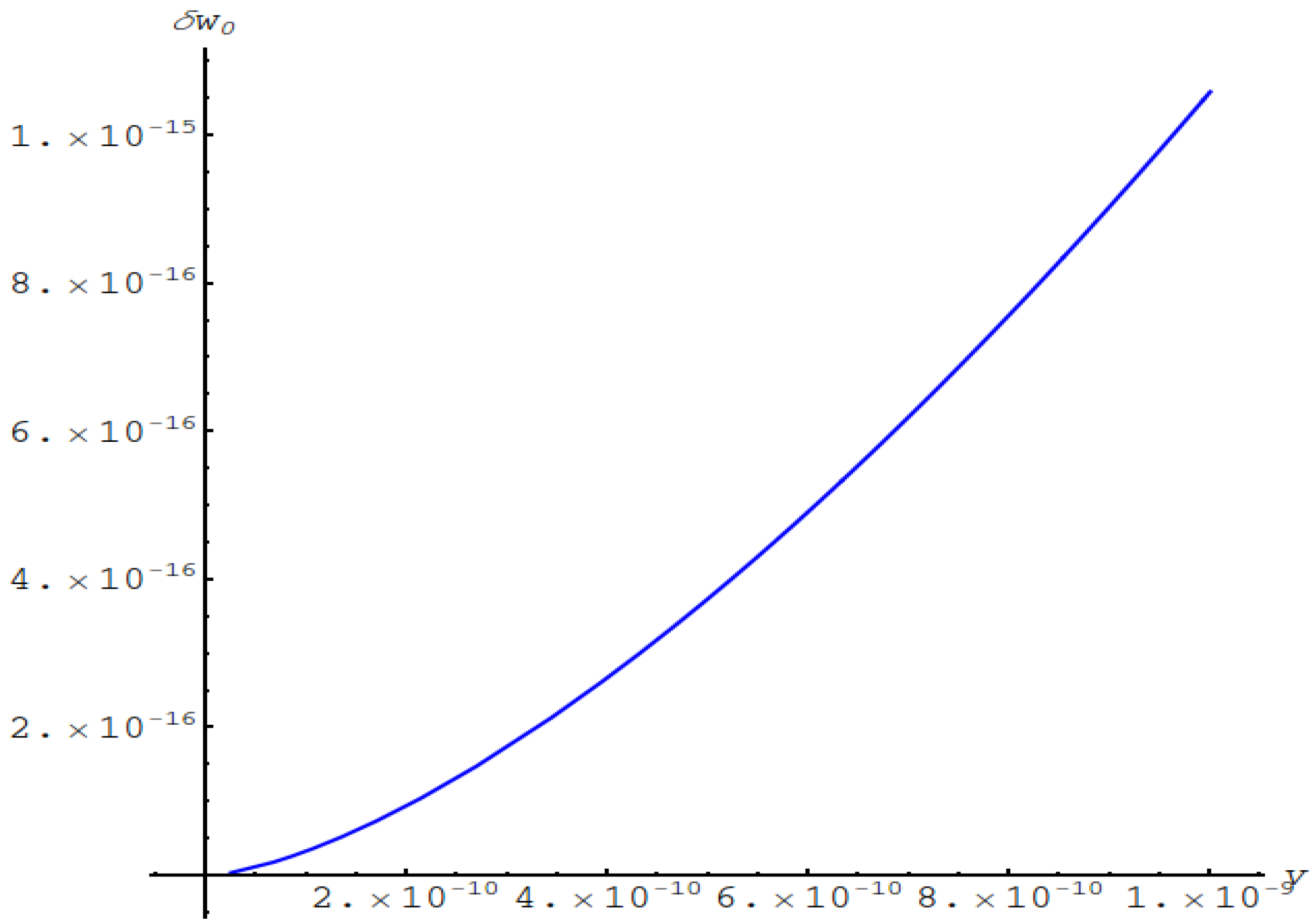
Figure 9 presents the dependence of the scaled amplitude δw₀ of the axial oscillations of the planetary orbit on the scaled radial coordinate v for the example where the heavier star mass μ′ = 100 and the lighter star mass μ = 1 in the units of the mass of the Sun. It shows that the amplitude of the oscillations is about quadrillion (!) times smaller than the interstellar distance. Thus, the system would be stable for a huge amount of time.

4. Non-Planar Motion of a Moon in a Star-Planet System

Kryukov and Oks [28] considered an example that included an Earth-like planet and a Sun-like star: the corresponding ratio of the masses μ/μ′ of the planet and the star is 3 × 10⁻⁶. The planet and the star are separated by the distance R = 1 a.u. There is also a moon moving in the vicinity of the planet.

The stable non-planar configuration is similar to that discussed in Section 2. The star here plays the role of the “heavier star” from Section 2. The planet here plays the role of the “lighter star” from Section 2. The moon plays the role of the “planet” from Section 2. The motion of the moon represents the rapid subsystem, while the rotation of the planet and of the star around their barycenter represents the slow subsystem.

Figure 10 displays the ratio Ω/ω of the frequencies of the rapid and slow subsystems versus the scaled projection w = z/R of the average plane of the moon’s orbit on the planet-star axis. It shows that in the range of 0 < w < 10^–4, the ratio of the frequencies is much greater than unity: the analytical method based on the separation of rapid and slow subsystems is applicable. (Figure 10, Figure 11, Figure 12 and Figure 13 are adopted from the paper by Kryukov and Oks [28]).

Figure 11 shows the scaled amplitude δw₀ of the oscillations of the moon’s orbit along the planet-star axis (the oscillations caused by the rotation of the star-planet subsystem) versus the scaled coordinate w = z/R. Analogously, Figure 12 displays the scaled amplitude δv of the oscillations of the scaled radius v = ρ/R of the moon’s orbit occurring in the plane perpendicular to the planet-star axis (the oscillations caused by the rotation of the star-planet subsystem) versus the scaled coordinate w.

Figure 13 presents the simulated 3D-trajectory of the moon. The coordinates (n, m, and w) are the scaled counterparts of the coordinates (x, y, and z).

Figure 11, Figure 12 and Figure 13 demonstrate that the conic-helical orbit of the moon in the star-planet-moon system will remain stable for a very long period of time. For the sake of clarity, the orbit is wound on the conical frustum such that the distance between the base of the cone and the cutting plane (parallel to base) is much smaller than the average diameter of the cone. We emphasize that a relatively distant star causes the following two effects: (1) The plane of the moon’s orbit will be perpendicularly oriented to the planet-star axis; (2) the trajectory of the moon becomes conic-helical.

5. Non-Planar Motion of a Circumbinary Planet

Schneider [31] and later Farago and Laskar [30] analytically studied a system consisting a circular binary and a planet in a non-planar motion. They assumed that the characteristic size A of the planetary orbit is much greater than the characteristic size a of the binary. Farago and Laskar [30] derived their analytical results by expanding the Hamiltonian in terms of the ratio a/A << 1. They found that the orbital plane of the planet precesses about the angular momentum of the binary.

Oks [29] showed the following: “There is also the precession of the orbital plane of the planet within the orbital plane… The frequency of this additional precession is not the same as the frequency of the precession of the orbital plane about the angular momentum of the binary, though the frequencies of both precessions are of the same order of magnitude”. Below are some of the details.

One part of the system under consideration is a circular binary star, the stars’ masses are M₁ and M₂ and the distance between them is denoted by a. They rotate with the following frequency.

Ω = [G(M₁ + M₂)/a³]^1/2

(14)

There is also a circumbinary planet in a non-planar motion. The major semi-axis A of its (approximately) elliptical orbit satisfies the following inequality.

A >> a.

(15)

In the first approximation, the planet revolves with the following frequency.

ω = [G(M₁ + M₂ + m)/A³]^1/2.

(16)

From Equations (14)–(16), the following is the case.

ω << Ω.

(17)

Based on this, Oks [29] wrote the following: “Thus, the circumbinary planet can be treated as a slow subsystem and the binary star can be treated as a rapid subsystem”.

The averaging over the rapid subsystem results in the following situation. The planet “feels” each star as a circular ring having the mass of the star uniformly distributed around the ring”.

The planet moves according to the following effective potential:

V_eff = −G(M₁ + M₂)/r − GMa²(3 cos²θ − 1)/(4r³),

(18)

where the reduced mass of the binary is as follows.

M = M₁M₂/(M₁ + M₂).

(19)

Oks [29] clarified: “The second term in the effective potential from Equation (18) is due to the quadripole interaction (the higher multipoles have been disregarded). The effective potential V_eff from Equation (18) is mathematically equivalent to the potential V_E for a satellite orbiting the oblate Earth (refer to, e.g., the book by Beletsky [39]). The latter is described as follows.

V_E = −GM_E/r − GM_E|I₂| R²(3 cos²θ − 1)/(2r³).

(20)

In Equation (20), R is the Earth radius at the equator, M_E is the mass of the Earth, and I₂ is a constant describing the relative difference between the polar and equatorial diameters of the Earth. The solution for the problem of a satellite orbiting the oblate Earth is well-known (refer to, e.g., the book by Beletsky [39]).

Based on this analogy, Oks [29] stated that the elliptical orbit of the planet is engaged in two kinds of precessions and they are described as follows.

The first precession is the precession of the orbit in its plane. The corresponding angular frequency is:

ω_{precession in plane} = (3/8)(a/p)²(1 − 5 cos²i)ωM₁M₂/(M₁ + M₂)²,

(21)

where the following is the case.

p = 2 r_min r_max/(r_min + r_max).

(22)

Here, r_max and r_min are the apoapsis and periapsis of the planetary orbit, respectively; i is the orbit inclination.

This precession is illustrated in Figure 14 (adopted from the paper by Oks [29]. It is the precession missed by Farago and Laskar [30].

Oks [29] noted that in Equation (21), 1 − 5 cos²i = 0 for i = 63.4 degrees and ω_{precession in plane} becomes zero. Thus, the circumbinary planet, with an orbit of this degree of inclination, does not experience the precession in the plane of the orbit.

The second precession is the precession of the planetary orbit plane around the angular momentum M of the binary with the following angular frequency:

ω_{precession of plane} = (3/4)(a/p)² (cos i)ωM₁M₂/(M₁ + M₂)²,

(23)

which is the same as the one discovered by Schneider [31] and Farago and Laskar [30]. It is observed that at i = 90 degrees, i.e., for the configuration where the orbital plane of the plane is orthogonal to the plane of the rotation of the binary, this precession vanishes.

We note that for the range of the inclination angles i < arccos[(3/5)^1/2] = 39 degrees, the Kozai–Lidov coupling of the inclination and the eccentricity of the planetary orbit is irrelevant. We also mention that for sufficiently high ratios of the frequencies Ω/ω of the rapid and slow subsystems (i.e., when Equation (17) is satisfied) and for the eccentricity of the planetary orbit that is not too close to unity, there will be practically no overlap of resonances of the two subsystems.

Oks [29] also noted the following: “The system under consideration is mathematically equivalent also to a highly-excited hydrogen atom in a linearly-polarized electric field of a high-frequency laser radiation E(t) = E₀ cos ω_Lt, where the Kepler frequency of the Rydberg electron is much smaller than the laser frequency ω_L. The latter problem has been treated analytically by Nadezhdin and Oks [40] by separating the rapid and slow subsystems”. They found that the atomic electron moves in the following effective potential (in spherical polar coordinates with the z-axis along vector E₀).

V_eff = −e/r − (γ/r³)(3 cos²θ − 1), γ = e³E₀²/(4m_e²ω⁴).

(24)

Here, e and m_e are the electron charge (by the absolute value) and the electron mass, respectively. One can observe that the effective potentials from Equations (18) and (24) are indeed mathematically equivalent.

Nadezhdin and Oks [40] also emphasized that the physical system described by the effective potential from Equation (24) possesses a higher geometrical symmetry. Indeed, the geometrical symmetry is axial (leading only to the conservation of M_z). Yet M² is also conserved (conserved exactly for the potential from Equations (18), (20), or (24) or conserved approximately if the higher multipoles would be taken into account). The conservation of M² is manifested by the fact that the shape of the elliptical orbit is not influenced by the perturbation (M² is proportional to the area of the elliptical orbit).

Only few physical systems are characterized by a higher geometrical symmetry. Therefore, the higher geometrical symmetry of a circumbinary planet under consideration is of general physical interest.

The assumption of the circular orbits of the stars in the binary was relaxed in Oks [34] paper. The corresponding results are presented in this review in Appendix A.

6. Circular Binary Star and an Interstellar Interloper

In this section, we follow the paper by Oks [32] and present a solution (obtained analytically) to the motion of a relatively distant interstellar interloper around a circular binary by using the same method as in Section 5. The system under consideration consists of a circular binary (the stars of the masses M₁ and M₂ at the distance a from one another) and a relatively distant interstellar interloper of the mass m₀ << (M₁ + M₂). The impact parameter b, which characterizes the trajectory of the interstellar interloper, satisfies the condition b >> a.

The Kepler frequency Ω of the stars’ rotation is given by Equation (14) from the previous section. The characteristic frequency of the “rotation” of the interstellar interloper reaches its maximum value at the distance r_min of the closest approach ω = v_max/r_min, where v_max is the interstellar interloper velocity at the closest approach.

For the interstellar interloper to represent the slow subsystem and for the binary to represent the rapid subsystem, the following obvious condition should be met: ω << Ω, which approximately corresponds to the requirement a << b.

Similarly to the interaction potential from Equation (18), the effective potential energy of the interstellar interloper is as follows:

U_eff(r, cos² θ) = −Gm(M₁ + M₂)/r − GmMa²(3 cos² θ − 1)/(4r³),

(25)

where

m = m₀(M₁ + M₂)/(m₀ + M₁ + M₂)

(26)

is its the reduced mass and M is given by Equation (19).

The geometrical symmetry of this system is axial (rather than spherical) since U_eff from Equation (25) depends on the polar angle θ. Nevertheless, similar to the situation described in Section 5, there is a higher geometrical symmetry: the square of the angular momentum is conserved in addition to the conservation of its projection on the axis of the rotation of the binary. Thus, the angle between the angular momentum vector and the axis of the symmetry is also conserved since the cosine of this angle is equal to the ratio of the angular momentum projection on this axis to the absolute value of the angular momentum.

Therefore, in the general non-planar configuration of this physical system and during its time evolution, the angular momentum vector, which is constant by magnitude, rotates about the axis of the symmetry while constituting the constant angle with this axis. This finding provides important information about the trajectory of the interstellar interloper on the general non-planar configuration.

Next, Oks [32] considered a particular situation with respect to the planar motion of the interstellar interloper when it moves in the plane of the binary rotation. After setting cosθ = 0 in U_eff from Equation (25), he obtained the following.

U_eff(r, 0) = −Gm(M₁ + M₂)/r + GmMa²/(4r³).

(27)

The analytical solution for motion described by the potential energy is as follows:

U(r) = –α/r + γ/r³, (α > 0, γ > 0),

(28)

where the second term is relatively minor compared to the first term and this is well-known (refer to, e.g., the book by Kotkin and Serbo [41]). The final result for the explicit expression for the trajectory by Kotkin and Serbo [41] can be rewritten for the interstellar interloper situation as follows.

p₁/r = 1 + e₁cos λφ + f cos 2φ

(29)

Here, the following is the case:

p₁ = p [1 + ε(e² + 2)],

(30)

where

e = [1 + 2EL²/(mα²)]^1/2

(31)

is the unperturbed eccentricity (hereafter, simply termed “eccentricity”),

p = L²/(mα)

(32)

is the unperturbed semi-latus rectum,

ε = G²m⁴M₁M₂a²/(4L⁴) << 1

(33)

is a dimensionless small parameter and the following is the case.

e₁ = e [1 + ε(3e⁴ − 2)/(2e²)], f = εe²/2.

(34)

The unperturbed eccentricity is e > 1 since the energy E of the interstellar interloper is positive.

For the unperturbed motion (i.e., at ε = 0) at infinity, 1 + e cos[φ₀(r = ∞)] = 0 (refer to Equations (29) and (34)) and the following is the case.

φ₀(r = ∞) = arccos(−1/e).

(35)

Since angle of deflection from the straight line is the following:

β = 2φ(r = ∞) − π,

(36)

then, for the unperturbed motion, the angle of deflection is as follows.

β₀ = 2 arccos(−1/e) − π.

(37)

For the perturbed motion, upon expanding the right side of Equation (29) in terms of the small parameter ε, one obtains the following.

1 + e₁cosλφ + f cos2φ ≈ 1 + e cosφ + ε s(e),

(38)

where the following equation results.

s(e) = 1/e² − 2e² + 1 − 3(e² − 1)^1/2arccos(–1/e).

(39)

In the limiting cases, the function s(e) is as follows:

s(e) ≈ –3π 2^1/2(e − 1)^1/2 at (e − 1) << 1 and s(e) ≈ −2e² at e >> 1.

(40)

Figure 15 shows the plot of this function. (Figure 15, Figure 16 and Figure 17 are adopted from the paper by Oks [32]).

Obviously at r = ∞, the right side of Equation (29) should vanish. Therefore, according to Equation (38), one obtains the following.

1 + e cosφ + ε s(e) = 0.

(41)

Thus, the cosine of the perturbed angle φ is expressed as follows.

cosφ = −[1 + ε s(e)]/e.

(42)

Upon substituting φ = φ₀ + Δφ in Equation (41), where |Δφ| << φ₀, one obtains the following.

Δφ = ε s(e)/(e² − 1)^1/2.

(43)

Consequently, according to Equation (36), for the perturbed angle of deflection from the straight line, one obtains the following:

β = 2(φ₀ + Δφ) − π = 2 arccos (−1/e) − π + ε u(e),

(44)

where the following equation results.

u(e) = 2s(e)/(e² − 1)^1/2.

(45)

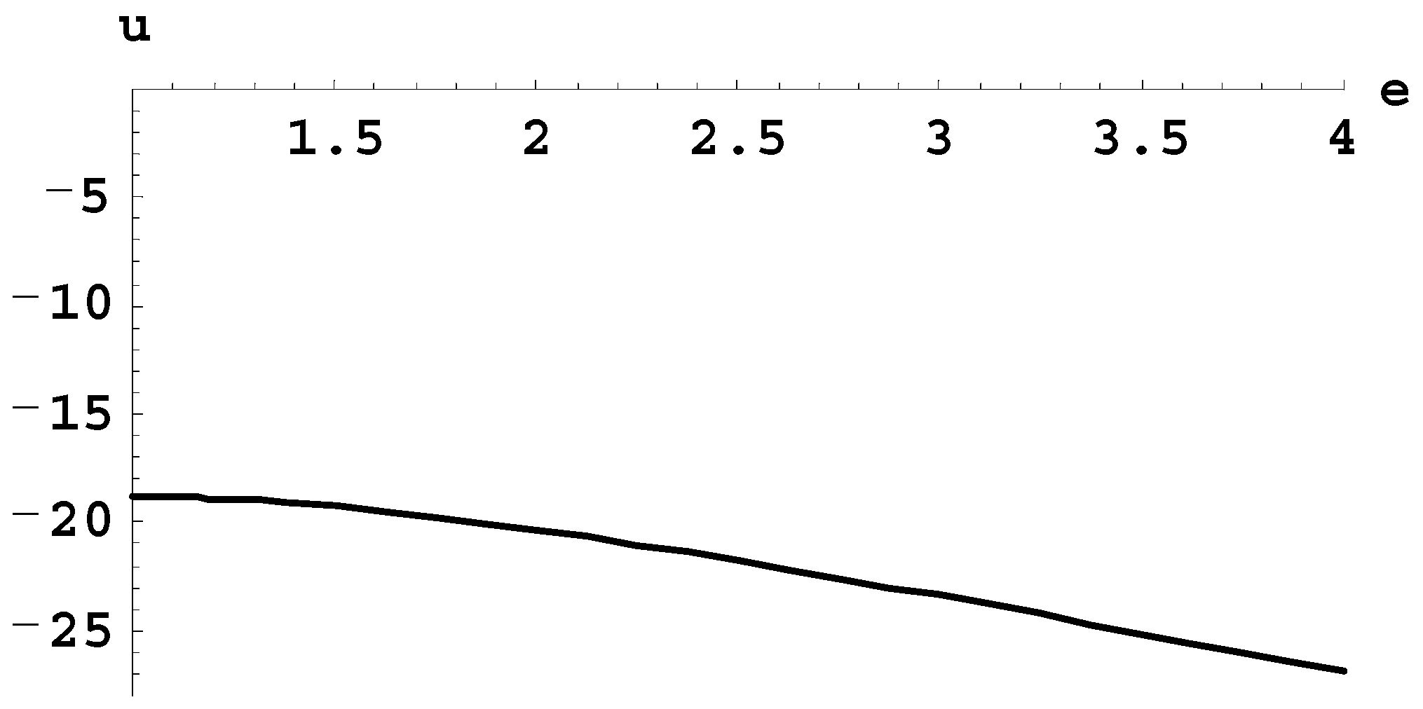
In the limiting cases, the function u(e), which controls the correction of the angle of deflection, simplifies as follows: u(e) = −6π –2^9/2(e − 1)^5/2/5 at (e − 1) << 1 and u(e) ≈ −4e at e >>1. Figure 16 displays the plot of the function u(e).

Therefore, the relative correction Δ to the deflection angle, defined as the ratio of the correction to the unperturbed value, has the following expression.

Δ(e) = ε w(e), w(e) = u(e)/[2arccos(−1/e) − π].

(46)

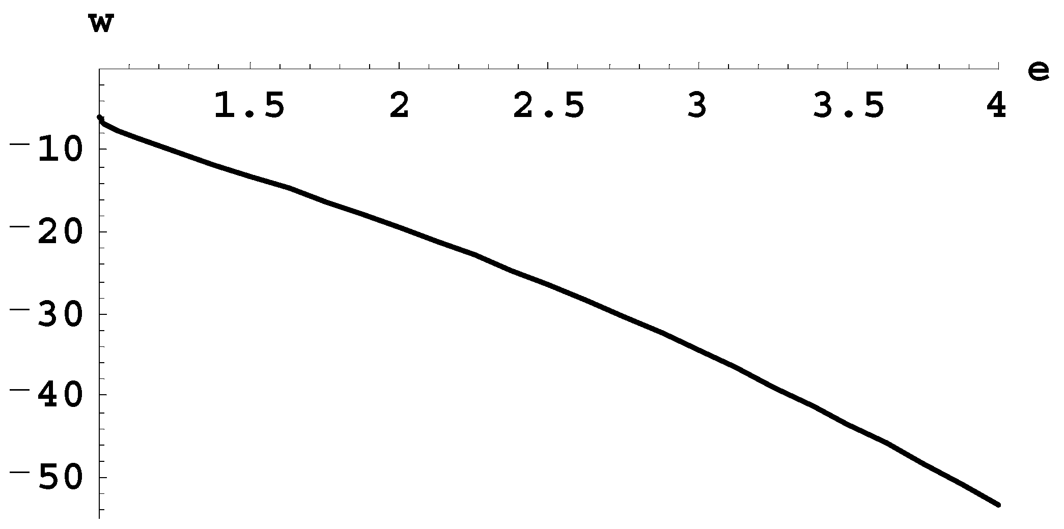
In the limiting cases, the function w(e), which controls the relative correction to the angle of deflection, simplifies to w(e) = −6 − 2^5/2 3(e − 1)^1/2/π at (e − 1) << 1 and w(e) ≈ −2e² at e >> 1. Figure 17 shows the plot of the function w(e).

The relative difference w(e) is presented in units of ε = G²m⁴M₁M₂a²/(4L⁴). From Figure 16 and Figure 17, one can observe that, in the three-body treatment, the angle of deflection of the interstellar interloper from the straight line decreases compared to the corresponding two-body approximation. It is observed that the greater the eccentricity, the greater (by the absolute value) the relative correction becomes.

The above results seem to have a fundamental importance, especially in view of the fact that two interstellar interlopers—Oumuamua and 2I/Borisov—have recently been found to travel through the solar system (refer to some of the latest papers; for instance, by Bodewits et al. [42], Zhang and Lin [43], and references therein). Thus, the above results should also further heighten the interest of the astrophysical community to interstellar interlopers in the Universe. From a practical point of view, one can determine the ratio m/L (characterizing the interloper) for the known eccentricity e by using our results: Indeed, the parameter ε (defined in Equation (33)), which controls the corrected angle of deflection in Equation (46), depends on the parameters of the interloper as being proportional to (m/L)⁴.

7. New Method for Detecting and Measuring Parameters a Compact Dark Matter Object Belonging to a Binary System

Compact dark matter objects (CDOs) have been the subject of many discussions in the literature (for the latest publications, refer to the papers by Errehymy et al. [44], Hadjimichef et al. [45], Raidal et al. [46], Dvali et al. [47], Horowitz et al. [48], Liao et al. [49], and the references therein). The mass and the distance of the CDOs are usually estimated via the gravitational microlensing effect. However, there are several shortcomings of this method (refer to the papers by Gilster [50], Griest et al. [51], and Hawkins [52]). One shortcoming is that the application of this method requires the alignment to be precise: Therefore, detections of CDOs by this method are rare and impossible to predict. Another shortcoming is that one should allow for competing background events: This makes a reliable detection very difficult.

Oks [33] suggested an alternative method for detecting and measuring parameters of dark matter objects. The method originates from the results presented in Oks [27] and by Kryukov and Oks [28], which are discussed above in Section 2

Oks [33] considered the following scenario: “There is a star of mass m. The star has one planet. The orbital plane of the planet does not contain the star. In other words, there is some distance z₀ between the star and the equilibrium position of the planetary orbital plane—see Figure 18 adopted from the paper by Oks [33]. This signifies the presence of a relatively distant gravitating object located at the z-axis at some (yet unknown) distance R from the star: R >> z₀. So, the object and the star constitute a binary system. If in the positive direction of the z-axis there is no visible star, this could signify that in this binary system, the companion of the star is a CDO”.

Oks [33] demonstrated a method for analytically obtaining the unknown mass M of the CDO and its unknown distance R from the star by employing the following input parameters: z₀, ρ₀ (the equilibrium radius of the planetary orbit), m (the star mass), and the orbital frequency F (or the orbital period T) of the planet. He introduced the scaled and dimensionless notations of the following:

w = z₀/R, v = ρ₀/R, b = M/m, f = F R^3/2/(Gm)^1/2_,

(47)

where F is the orbital frequency of the planet. The scaled orbital frequency f of the planet takes the following form.

f = (1 − w)^–1/2(w² + v²)^−3/4.

(48)

From Equations (47) and (48), one obtains the following.

F = (Gm)^1/2/[(1 − z₀/R)^1/2 (z₀² + ρ₀²)^3/4].

(49)

Equation (49) can be solved for the only one unknown quantity, R, to yield the following.

R = z₀/{1 − Gm/[(z₀² + ρ₀²)^3/2F²]}, F = 2π/T.

(50)

It is observed that the unknown distance R between the CDO and the star can be determined by means of Equation (50).

In the next step, one can use Equation (3) from Section 2 (for the scaled equilibrium radius v(w, b) of the planetary orbit) to find out the sole remaining unknown quantity b = M/m, while employing the definitions of w and v from Equation (47).

M = m[z₀/(R − z₀)][(R − z₀)² − ρ₀²]^3/2/(z₀² + ρ₀²)^3/2.

(51)

Since the separation R between the CDO and the star has already been found by employing Equation (50), Equation (51) can be used for determining the last still unknown quantity: the CDO mass M.

Oks [33] provided the following numerical example: “If z₀ = 1/1000 a.u., ρ₀ = 1/10 a.u., m = M_Sun/2 (M_Sun being the solar mass), and the planet has the orbital period T of 49/3 days, then from Equation (50) one obtains (after converting the input data into the cgs units) the separation between the CDO and the star: R = 7.49 a.u. Finally, from Equation (51) one gets the CDO mass: M = 56.1 M_Sun”.

It should be noted that for the numerical data chosen as an example, the frequency of the rotation of the star and the CDO about their barycenter is smaller than the orbital frequency of the planet by two orders of magnitude. Thus, the condition for the separation of the rapid and slow subsystems in order to be legitimate is satisfied.

The proposed method should be useful, in particular, for obtaining additional observational data on the CDOs and, therefore, on dark matter in general.

8. Circular Sitnikov Problem in a More General Setup

Studies of the “orthogonal” configuration of the restricted three body problem that are initiated by Sitnikov [53], e.g., the motion of a planet along the line that is perpendicular to the orbital plane of two stars in the binary and that crosses the barycenter of the binary (the z-axis), possess an interesting particular case where the stars in the binary move in circular orbits: the circular Sitnikov problem. Analytical solutions, expressed as a one-fold integral, had been previously obtained by Pavanini [54] and MacMillan [55] for the special case of the circular Sitnikov problem where the two stars are of equal masses. References on subsequent studies can be found, e.g., in the book by Dvorak and Lhotka [56] and in the papers by Sidorenko [57] and by Abouelmagd et al. [20].

In particular, in 1994 Belbruno et al. [35] completed the integration (not performed by Pavanini [54] and MacMillan [55]) and obtained, e.g., the following exact analytical result for the period of oscillation of the planet for the special case of the circular Sitnikov problem where the two stars are of equal masses:

T = [2^1/2/(1 − 2k²)]{E(k) + [π/(2^3/2(1 − 2k²)^1/2)][1 − Λ₀{arcsin[(1 − 2k²)/(1 − k²)]^1/2, k}],

(52)

where E(k) is the complete elliptic integral of the second kind and Λ₀(ϕ, k) is the Heuman Lambda function. In Equation (52), the quantity k is related to the dimensionless energy h of the planet as follows.

k = (2 + h)^1/2/2.

(53)

The units of h are chosen such that the bound motion corresponds to the range.

−2 < h < 0.

(54)

The corresponding scaled potential energy has the following form:

V = −2/(1 + 4z²)^1/2,

(55)

where z is the scaled dimensionless coordinate in units of the separation between the two stars.

For a more general setup of the circular Sitnikov problem where the two stars in the binary have, generally speaking, unequal masses M₁ and M₂, an approximate analytical solution based on the separation of rapid and slow subsystems was presented in Appendix A of the paper by Oks [34]. Here are some of the details.

The starting point was the physical situation from the Oks [34] paper, which is also described in Section 5 of the present review. After averaging over the rapid subsystem (over the motion of the stars), the planet perceived each star as a circular ring possessing the mass of the star uniformly distributed around the ring. In this situation, the effective potential energy V_eff was given by Equation (18) for an arbitrary polar angle coordinate of the planet.

The linear motion of the planet along the z-axis corresponds to θ(t) = 0. Equation (18) then simplifies as follows.

V_eff(z) = −Gm(M₁ + M₂)/|z| − GmMa²/(2|z|³).

(56)

From the equation for the total energy E, where E < 0, the following was found.

dz/dt = ±(2/m)^1/2[|U_eff(z)| − |E|]^1/2

(57)

Thus, the solution for the equation of the motion has the form of the following one-fold integral.

t = ±(m/2)^1/2 ∫ dz/[Gm(M₁ + M₂)/|z| + GmMa²/(2|z|³) − |E|]^1/2

(58)

In that paper, the author introduced the following dimensionless quantities.

u = |z||E|/[Gm(M₁ + M₂)], b = Ma²E²/[2m²G²(M₁ + M₂)³].

(59)

Obviously, the parameter b is the square of the scaled total energy. Equation (58) has been represented in the following form.

t = ±[G(M₁ + M₂)m^3/2/(2^1/2|E|^3/2)] ∫ du/(1/u + b/u³ − 1)^1/2 =
 ± [G(M₁ + M₂)m^3/2/(2^1/2|E|^3/2)] ∫ du u^3/2/(b + u² − u³)^1/2.

(60)

The expression for the turning points ±u₀ was obtained by solving the equation u³ − u² − b = 0.

u₀ = g(b) = 1/3 + 2^1/3/{3[2 + 27b + 3^3/2(4b + 27b²)^1/2]^1/3} + [2 + 27b + 3^3/2(4b + 27b²)^1/2]^1/3/(2^1/33).

(61)

Figure 19 presents the plot of the function g(b).

The analytical result for the period T of the motion is the following:

T = [2^3/2G(M₁ + M₂)m^3/2/|E|^3/2] f(b) = {(2M₁M₂)^3/4a^3/2/[G^1/2(M₁ + M₂)²]}f(b)/b^3/4,

(62)

where

$$\mathrm{f}\left(\mathrm{b}\right)={\displaystyle \underset{0}{\overset{\mathrm{g}(\mathrm{b})}{\int }}{\mathrm{du}\mathrm{u}}^{3/2}}/{\left({\mathrm{b}+\mathrm{u}}^2-{\mathrm{u}}^3\right)}^{1/2}.$$

(63)

For b << 1, one obtains the following.

f(b) ≈ π/2.

(64)

Equation (62) can be represented in the following form:

T_s(b) = f(b)/b^3/4, T_s = TG^1/2(M₁ + M₂)²/[(2M₁M₂)^3/4a^3/2],

(65)

where T_s is the scaled period.

Figure 20 demonstrates the dependence of the scaled period T_s on b (i.e., on the scaled square of the energy). It shows that the period of the oscillations decreases as the absolute value of the energy increases.

From Equation (64), it follows that for b << 1 one obtains the following.

T_s ≈ π/(2b^3/4).

(66)

Since b is proportional to E², this means that for relatively small energies, the period is inversely proportional to 1/E^3/2 and, thus, obeys the corresponding Kepler law. This should be expected: For relatively small energies, the situation approaches the case where the planet moves in the gravitational field of a “single” star of the mass (M₁ + M₂).

For the special case of M₁ = M₂, i.e., for the only case in which Belbruno et al. [35] obtained the analytical result for the period (given by Equation (52)), it would be instructive to compare the latter to the corresponding result from the Oks paper [34]. The parameterizations in the papers by Belbruno et al. [35] and by Oks [34] were very different from one another. The meaningful comparison (i.e., comparing “apples to apples”) can be performed for the following quantity.

$$\mathrm{S}\left(\left|\mathrm{h}\right|\right)={\left|\mathrm{h}\right|}^{3/2}\mathrm{T}\left(\left|\mathrm{h}\right|\right)/\left\{\underset{\mathrm{h}\to 0}{\lim }\left[{\left|\mathrm{h}\right|}^{3/2}\mathrm{T}\left(\left|\mathrm{h}\right|\right)\right]\right\}$$

(67)

(We note that the scaled energy h is negative for bound states in the notations from Belbruno et al. paper [35]).

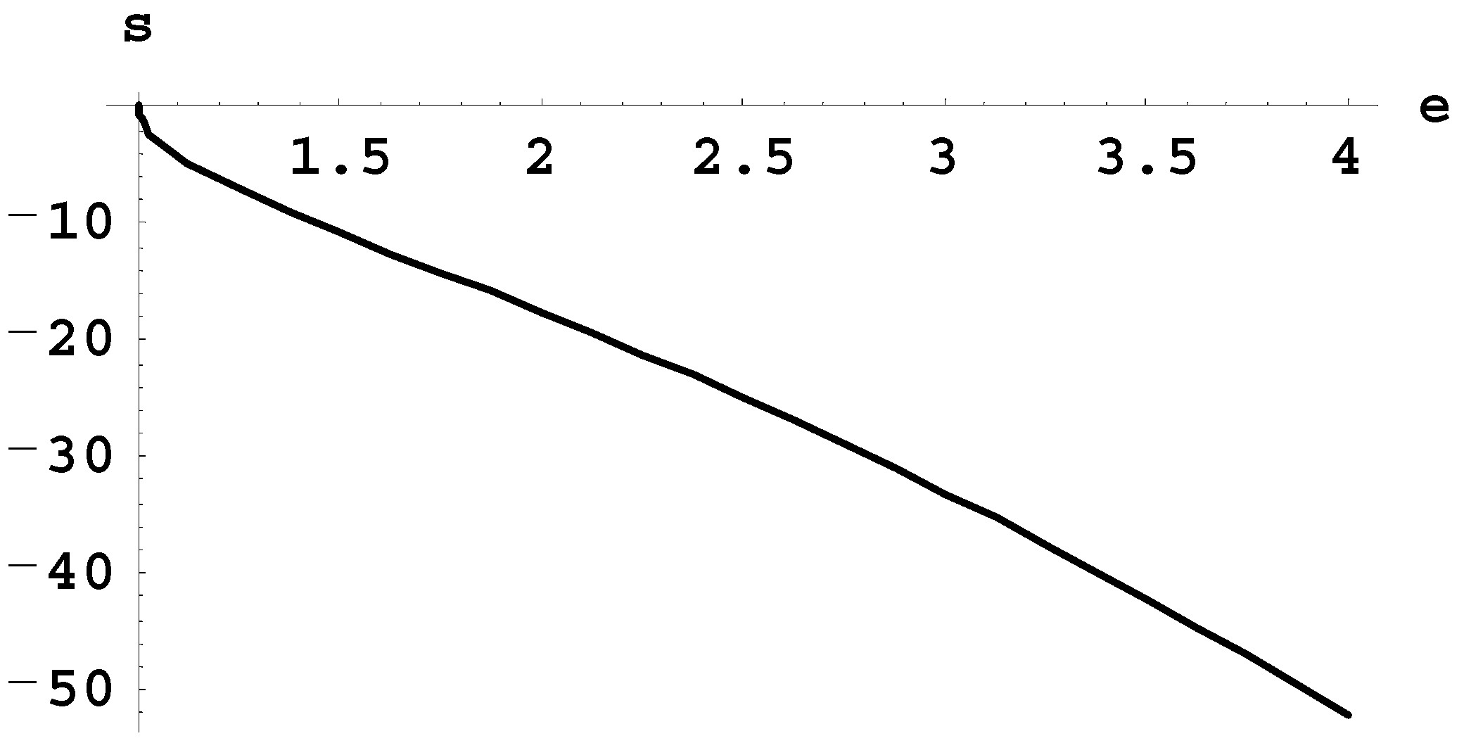
In Figure 21, the results for S(|h|) in this special case (M₁ = M₂) by Oks [34] and by Belbruno et al. [35] are shown by the solid and dashed lines, respectively, for the range of the applicability of the Oks results [34] (i.e., for the relatively large amplitude of the oscillations corresponding to the relatively small absolute value of the scaled energy h).

It can be observed that, for this special case (M₁ = M₂), the approximate analytical result for S(|h|) by Oks [34] is in good agreement with the analytical result of S(|h|) by Belbruno et al. [35].

It should be emphasized that for the more general setup where the masses of the stars in the binary are not equal, the approximate analytical result by Oks [34], obtained by separating rapid and slow subsystems, does not have the corresponding analytical results in the literature to the best of our knowledge.

For the sake of completeness, we note that for the opposite asymptotic case, where (h + 2) << 1, the analytical result for the period T of the oscillations can be obtained (without resorting to the rotating reference frame used by Belbruno et al. [35] by reducing the problem to an anharmonic oscillator. This is presented in Appendix B of the current review where, in particular, it was shown that there seems to be an error in the analytical calculation of the period of the oscillations by Belbruno et al. [35] or at least in their analytical calculation of the derivative dT/dh at h = −2.

9. Concluding Remarks

Most of the analytical results in the restricted three-body problem in celestial mechanics that were obtained before 2015 were limited to planar geometry, to the motion around the Lagrange points, or to the Kozai–Lidov effect. Recent advances in the analytical solutions of the non-planar restricted three-body problem, of which the present review is devoted to, opened up new avenues in this research area.

One of the analytical advances covered in this review is the discovery of conic-helical orbits of the light body in three body systems. Examples are presented for the motion of a planet around a binary star and for the motion of a moon in the planet-star systems.

Another analytical advance concerned the motion of a circumbinary planet in which its average distance from the binary is much greater than the distance between the stars. In addition to the previously known precession of the plane of the planetary orbit about the axis of the rotation of the binary, it was simultaneously shown that there is also a precession of the planetary orbit in its own plane.

For an interstellar interloper moving at a relatively large distance from a binary star, its angle of deflection from the straight line has been analytically calculated. This result permits the determination of the ratio of the mass to the angular momentum of the interstellar interloper.

This review also covered an alternative method for detecting and measuring parameters of compact dark matter objects (CDOs) that affect a star-planet system. The method permits the determination of the separation between the CDO and the star as well as the CDO mass.

Finally, analytical results on the circular Sitnikov problem were presented in a more general setup. Compared to the previous analytical results derived only for the special case of the equal masses of the two primary bodies, the presented results were obtained for the arbitrary ratio of the masses of the two primary bodies. The two primary bodies were considered to be stars in the binary, while the third (light) body was considered to be a planet. The most important result was obtained for the period T of the oscillations of the planet in this three-body system. For the special case of equal masses of the stars in the binary, this analytical result was compared to the corresponding analytical result by Belbruno et al. [35]. It was shown that there appears to be an error in the analytical calculation performed by Belbruno et al. [35] concerning the derivative dT/dh at h = −2 (where h is the scaled energy of the planet): in other words, at the relatively small amplitude of the oscillations of the planet.

We hope that the present review would motivate the search for further analytical solutions of the non-planar restricted three-body problem in celestial mechanics.