Optimisation of Imaging Confocal Microscopy for Topography Measurements of Metal Additive Surfaces

Abstract

Additive manufactured surfaces, especially metal powder bed fusion surfaces, present unique challenges for measurement because of their complex topographies. To address these measurement challenges, optimisation of the measurement process is required. Using a statistical approach, sensitivity analyses were performed on measurement settings found on a commercial programmable array scanning confocal microscope. The instrument measurement process parameters were compared by their effects on three quality indicators: the areal surface texture parameter Sa, measurement noise, and number of non-measured points. An analysis was performed using a full factorial design of experiments for both the top and side surfaces of test surfaces made from Inconel 718 and Ti-6Al-4V using powder bed fusion. The results indicated that measurements of metal additive surfaces are robust to changes in the measurement control parameters for Sa, with variations within 5% of the mean parameter value for the same objective, surface, and measured area. The number of non-measured points and the measurement noise were more varied and were affected by the choice of measurement control parameters, but such changes could be predicted by the statistical models. The contribution offered by this work is an increased understanding of imaging confocal microscopy measurement of metal additive surfaces, along with the establishment of good practice guidance for measurements.

1. Introduction

Surface topography measurement plays a vital role in metal additive manufacturing (AM) for assessing the surface texture to meet manufacturing requirements, and as a tool to investigate how a manufacturing process produces a surface and its topographic structures (features) [1,2,3,4]. These features that are present on a surface relate to the manufacturing process itself [4,5], but they can also lead to measurement challenges [2]. These challenges are due to the non-uniform nature of the optical properties on a surface (such as varying reflectivity) and the presence of high-aspect-ratio features, high slope angles, and undercuts, which all vary depending on the build orientation, powder size, and AM build process parameters [6].

To attempt to overcome these measurement challenges and improve the quality of measurement, optimisation of the measurement process is required. This optimisation has been performed for various measurement systems for metal powder bed fusion (PBF), including coherence scanning interferometry [7], focus variation (FV) [8], and X-ray computed tomography [9,10]. Surface topography measurement for metal PBF plays a significant role in understanding the manufacturing process through the measurement and assessment of surface texture and the features on the surface. Imaging confocal microscopy has been used to measure AM surfaces [11,12], with newer confocal systems being better able to overcome some of the challenges presented by metal PBF surfaces [12,13]. Additional developments in “confocal fusion” [13], which uses confocal microscopy and FV together to provide greater coverage in the final measurement result, have also been used to measure metal AM surfaces [14]. To achieve optimal setup configurations for these surface texture measurement systems, understanding of the measurement principles and the sensitivity of the measurement process parameters in the final measurement result is required. While much research has been undertaken in the field of surface texture measurement, generally (and in confocal microscopy, more specifically), there have not yet been many studies performed to understand the complex interaction between the confocal instrument and metal AM surfaces. A number of studies [15,16] have shown that this interaction requires further investigation, and that the current lack of available good practice guidance can result in measurement errors. We seek to address that issue in this paper. A deeper understanding of the sensitivity of these measurement parameters to metrics for quality is the basis of the contribution to science presented in this paper, with the conclusions intended to contribute to good practice guidance for the measurement of metal PBF using confocal microscopy.

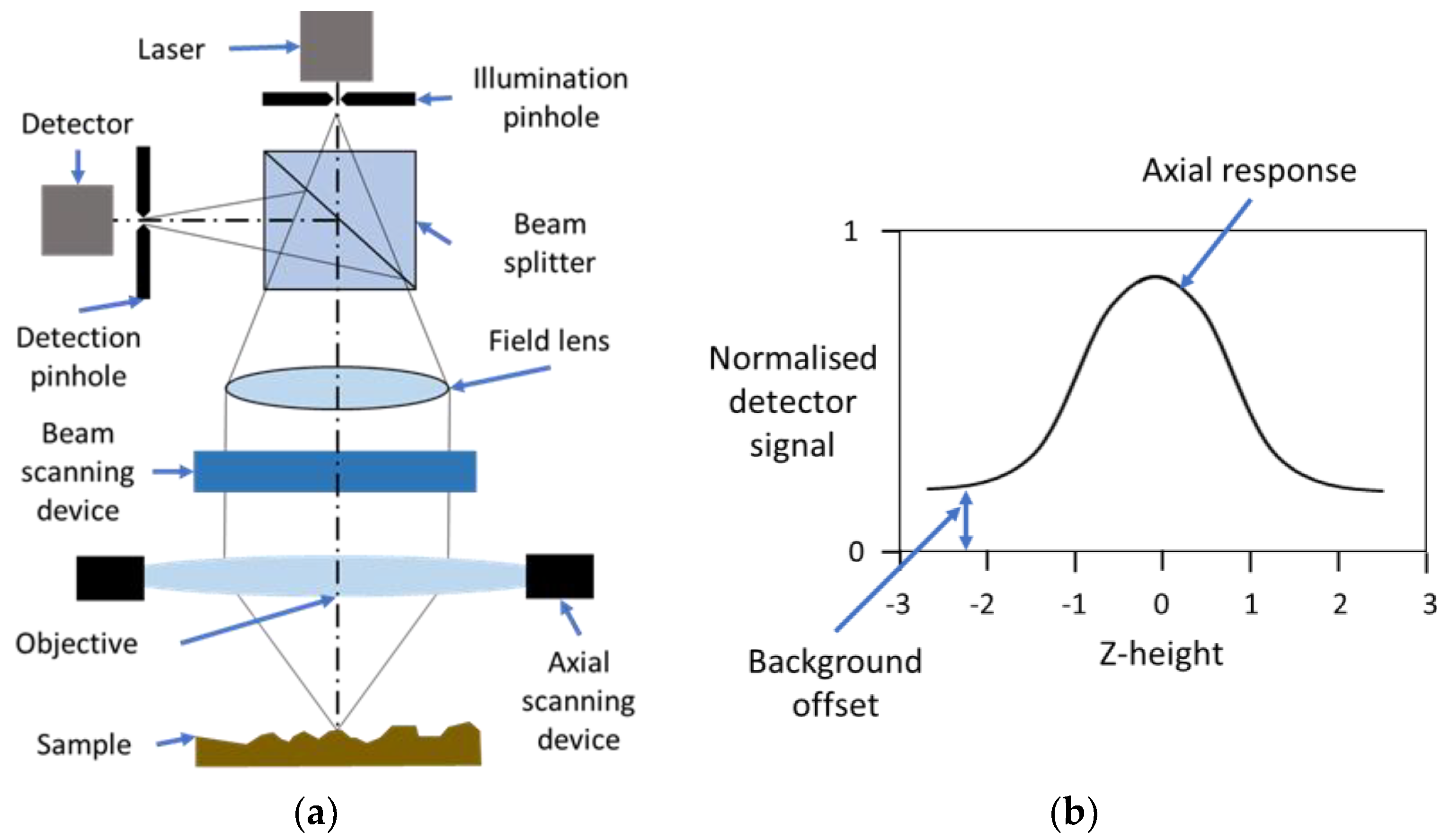
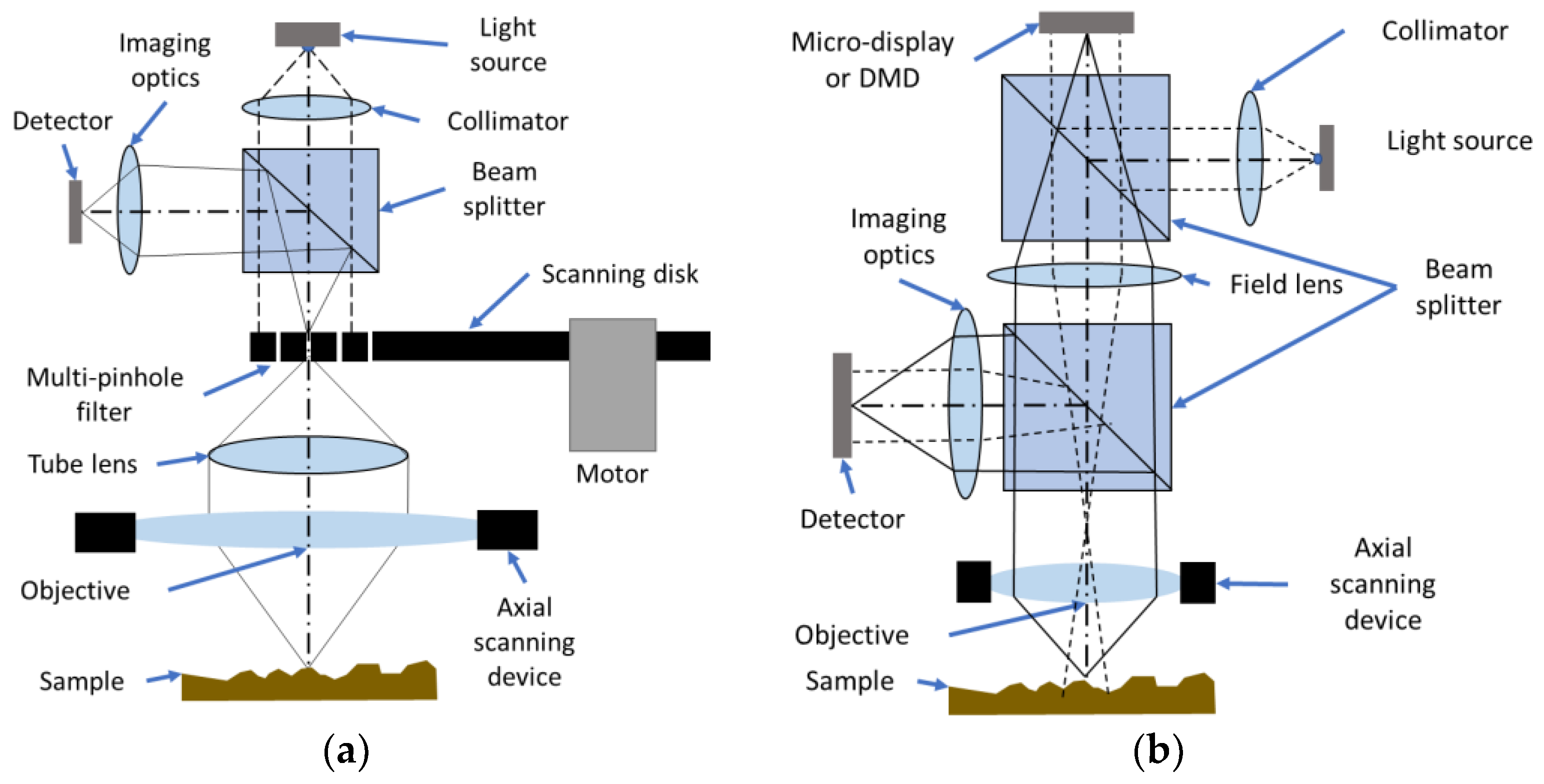
Background on Confocal Microscopy Techniques

In confocal microscopy (CM), intensity is used to determine topographic heights on a surface. By observing light that is reflected on a test surface under restricted illumination, optical section images can be produced at different vertical positions, with the highest intensity of signal for a lateral position coinciding with the surface height point [17,18]. In this work, we used imaging confocal microscopy [19], as opposed to “chromatic” confocal microscopy [20,21]. While chromatic confocal systems are used for surface measurement, they are less commonly used for additive surfaces, as their achievable accuracy is lower and they generally have poorer slope measurement capability [20]. There are several types of CM, typically laser scanning CM (LSCM), disk scanning CM (DSCM), and programmable array scanning CM (PACM) (see [17] for details).

In LSCM, a laser beam illuminates a pinhole within the optical axis, which is used to determine an intensity point on the confocal image from the reflection of the test surface at the focal plane of the objective [19]. Reflected light from the test surface passes back through the objective onto a second pinhole placed at a conjugate position to the illumination pinhole. Behind the detection pinhole is a detector that records the intensity of light that is reflected by the surface. Light reflected from out-of-focus positions on the surface leads to low-intensity signals at the detection plane. Conventionally, beam scanning devices use two galvanometric mirrors that move in discrete steps to measure across the x- and y-axes of the surface topography measurement, with bias on one of these axes to raster scan the points of the imaging plane. The operating principle and general configuration of an LSCM system are shown in Figure 1 [19].

In Figure 1a, the various components of the measurement technology are shown, where the beam scanning device will raster scan a laser point over the surface to produce a confocal intensity image, which is repeated for each vertical position in the scan to produce a vertical stack of confocal images [19]. In Figure 1b, the graph shows how for each measurement point on the topography, a height point can be determined by finding the peak axial response across the vertical stack of confocal images.

For DSCM and PACM, the measurement principle using pinholes and the measured intensity of the signal is the same, but they use a two-dimensional imaging detector—typically a charge-coupled device (CCD) or complementary metal–oxide–semiconductor (CMOS) sensor [19]. DSCM uses a spinning disk with a pattern of pinholes to allow for multiple points to be recorded at high frame rates, increasing the speed of measurement (see Figure 2a). Each pinhole acts as an illumination and detection element, as the light that is transmitted through the pinholes is focused onto the detector. The result is an optically sectioned image, which requires vertical stepping to scan the height range of the surface [19].

PACM, as shown in Figure 2b, uses an active micro-display to create patterns for illumination and detection [19]. In an illumination and detection mode, the operation is similar to that of DSCM, but with the disk replaced by the micro-display. Each pixel of the micro-display acts as an illumination and detection element at the same time, allowing for high-speed imaging and adjustable scanning methods (compared to a fixed physical disk), but PACM often has lower scanning speeds [19].

In this work, a variety of settings for a PACM system, common to other systems, are subjected to a sensitivity analysis to understand the effects of changing measurement parameters on the instrument. It is hoped that many of the conclusions—or at least the methods used to reach the conclusions—from this study can also be applied to LSCM and DSCM.

2. Materials and Methods

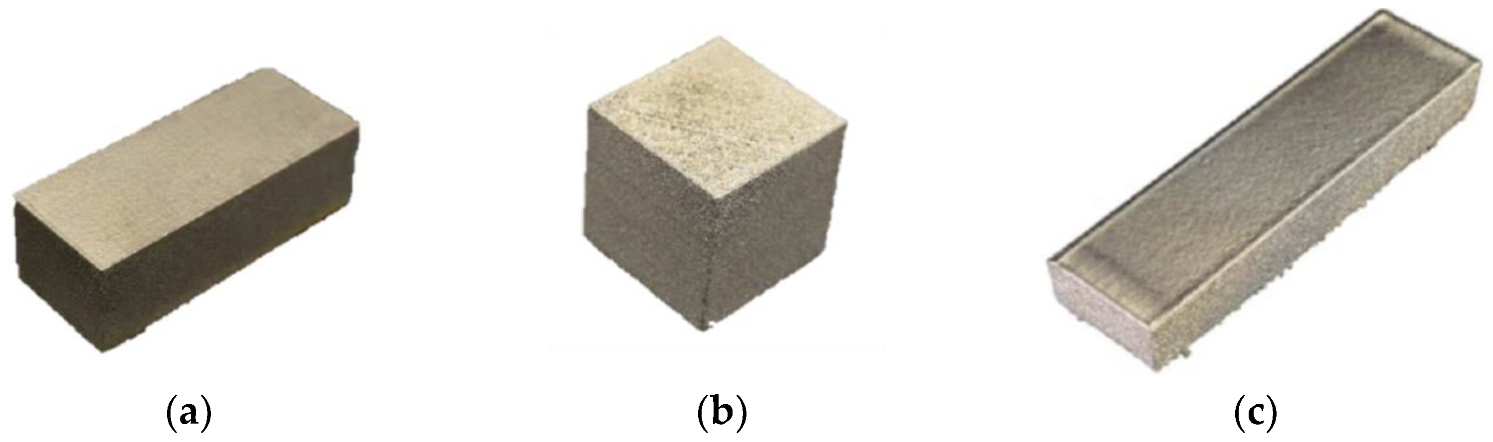
2.1. Test Artefacts

Three test artefacts produced by laser powder bed fusion (PBF-LB) and electron beam powder bed fusion (PBF-EB) were inspected (these were the same test artefacts that were used in a previous work with FV microscopy, and their specific production details are covered in

Table 1. Measurement process parameters and their levels.

Objective Magnification	10× NA: 0.3 FoV: (1.6 × 1.4) mm Optical Resolution: 0.47 µm	20× NA: 0.45 FoV: (0.8 × 0.7) mm Optical Resolution: 0.31 µm	50× NA: 0.8 FoV: (0.3 × 0.3) mm Optical Resolution: 0.18 µm
Scanning modes	CSSS CSDS	CSSS CSDS	CSSS CSDS
Lateral sampling resolution	Low—512 pixel (2.76 µm) High—1024 pixel (1.38 µm)	Low—512 pixel (1.38 µm) High—1024 pixel (0.69 µm)	Low—512 pixel (0.55 µm) High—1024 pixel (0.28 µm)
Vertical scanning rate	Low—1× (2 µm) Medium—2× (4 µm) High—4× (8 µm)	Low—1× (1 µm) Medium—2× (2 µm) High—4× (4 µm)	Low—1× (0.2 µm) Medium—2× (0.4 µm) High—4× (0.8 µm)
HDR	On Off	On Off	On Off
Threshold level	Low—5% Medium—3% High—1%	Low—5% Medium—3% High—1%	Low—5% Medium—3% High—1%

of [8]). The top surfaces were built perpendicular to the build direction. The test artefacts can be seen in Figure 3.

Using methods presented in an earlier work [8], the surface texture of the three test artefacts was preliminarily assessed via the ISO 21920 part 2 [22] Ra parameter—the arithmetic mean deviation of the assessed profile—using a contact stylus instrument. This comparison represents a simple “sanity check” that the confocal instrument (which uses physics that is generally difficult to model) is performing similarly to a contact system (which is much easier to model and not subject to the optical effects that may cause issues in the confocal measurement).

2.2. Confocal Microscopy Measurement Process Parameters

The test surfaces were measured using a Sensofar S-Neox [23]. The following measurement process parameters, some of which are common across confocal instruments, were considered:

• Objective magnification and numerical aperture (NA) [24];
• Scanning mode [17];
• Lateral sampling resolution [25];
• Vertical scanning settings [26];
• High dynamic range (HDR) [19];
• Threshold level [19].

Objective magnification refers to the optics under consideration; each has magnification, an NA, and a field of view (FoV) [24]. These values will influence the optical resolution and the slope limitation when measuring a single measurement area and, by extension, the total measurement area. These parameters, in turn, influence whether stitching is required to match a desired total measurement area. The S-Neox uses a series of aligned, parfocal objective lenses, so no movement of the sample or instrument is required when changing between lenses to acquire measurements of the same surface topography.

Scanning modes within this confocal instrument are configurations of projections that use a programmable array to imitate a Nipkow disk [17]. The system synchronises the programmable array and the CMOS sensor to create a confocal image at each z-position. There are two settings in the confocal instrument being considered:

• Coarse-shift single sampling (CSSS) creates projected slits in the programmable array, vertically spaced four pixels apart, that shift horizontally four times to produce each confocal image [17];
• Coarse-shift double sampling (CSDS) creates projected slits in the programmable array in two orientations (both four pixels apart) that scan in two directions: vertical slits that shift horizontally four times (as in CSSS), followed by horizontal slits that shift vertically four times. The responses for the horizontal and vertical scans are combined to produce the confocal image of intensities. Use of the CSDS setting results in increased measurement times but benefits from increased sampling within the same measurement [17].

The lateral sampling resolution setting refers to the number of points (or point spacing) in the final measured topography [25]. For the confocal instrument, the highest resolution corresponds to one measurement point per pixel on the detector, with lower resolutions achieved by decimating, i.e., taking every other detector pixel as the measured point. Each subsequent resolution setting will take half the number of points over the lateral axes in the final measured topography dataset, reducing the equivalent resolution.

The vertical scanning rate refers to the distance between images on the vertical axis; vertical scanning is not performed in a continuous mode, so as to allow for comparison of the scanning settings when using the HDR setting [26]. With a relative scanning range fixed for all test surfaces, this represents the number of images taken and influences the total measurement time, although this might be reduced in practice by more accurate positioning of the measurement volume.

HDR uses multiple exposures collected in sequence, with varying illuminations or exposure times, to create a composite image from the image data [19]. The HDR setting optimises the measurement for surfaces with a large variation in reflectance and/or slope, reducing the number of non-measured points. This setting increases the total measurement time by a factor equal to the number of light levels used.

The threshold level refers to an internal algorithm that acts to increase or decrease the system’s sensitivity to the optical signal to remove excessive noise (in the form of spikes in the data) over a certain size; the lower settings allow more noise points into the resultant topography, with higher values acting more harshly to remove data points [19]. This setting assesses the signal quality (i.e., the quality of the maximum signal of the axial response, as shown in Figure 1) to decide whether to calculate a peak position or classify a missing point, with a focus on targeting the common optical features present in CM.

2.3. Design of Experiments

The work performed in this paper follows a “design of experiments” approach [27]; the specific variables examined are presented in Table 1. In the analysis, the objective magnifications are “blocked” so that only the same objective can be compared for the different surfaces.

2.4. Performance Metrics

To assess the performance of the measurements, qualitative assessment was performed on the topography models that were reconstructed from the height maps. In addition, three measurement parameters were chosen to allow for a quantified comparison: measurement noise, percentage of non-measured points, and surface texture parameter Sa on the levelled surface topography.

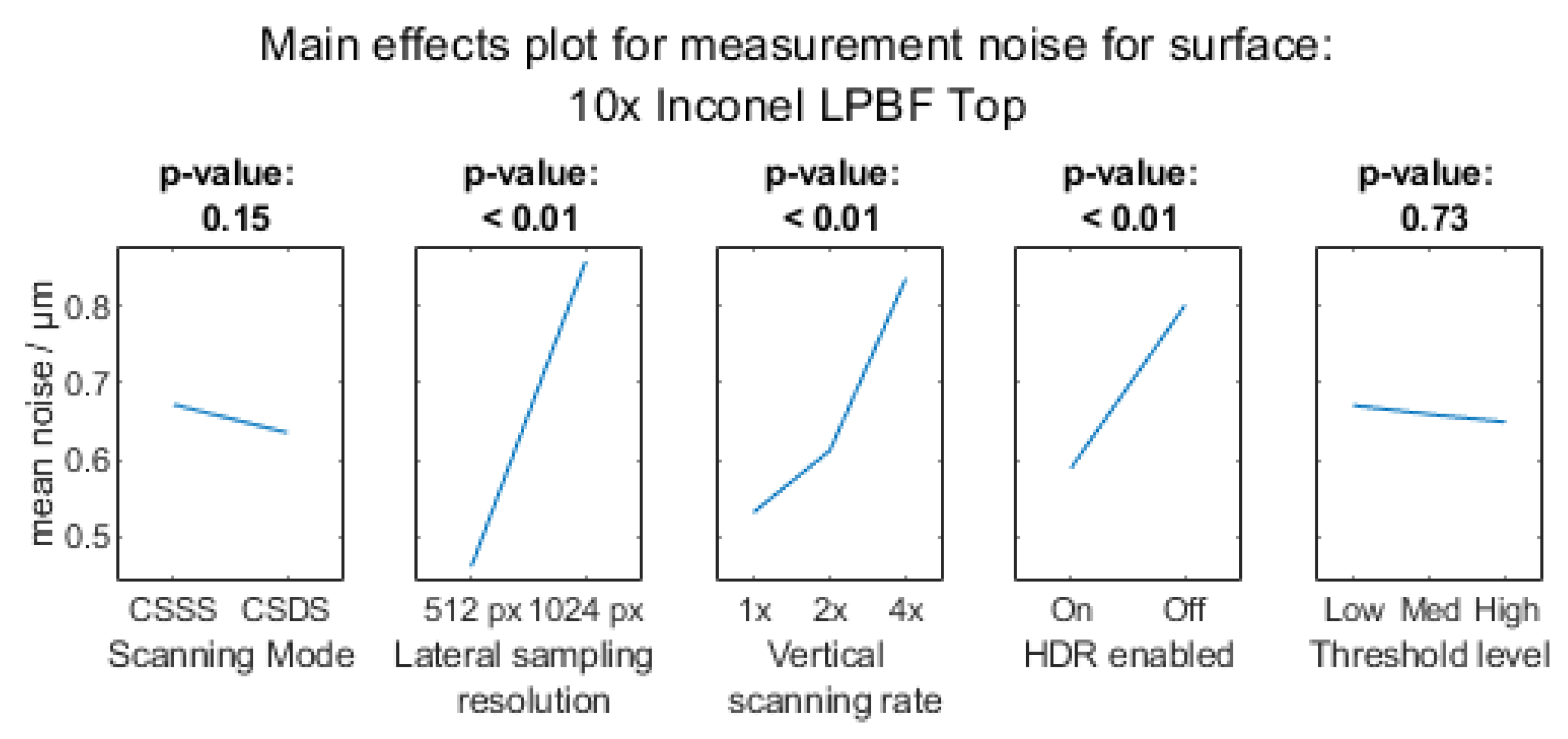
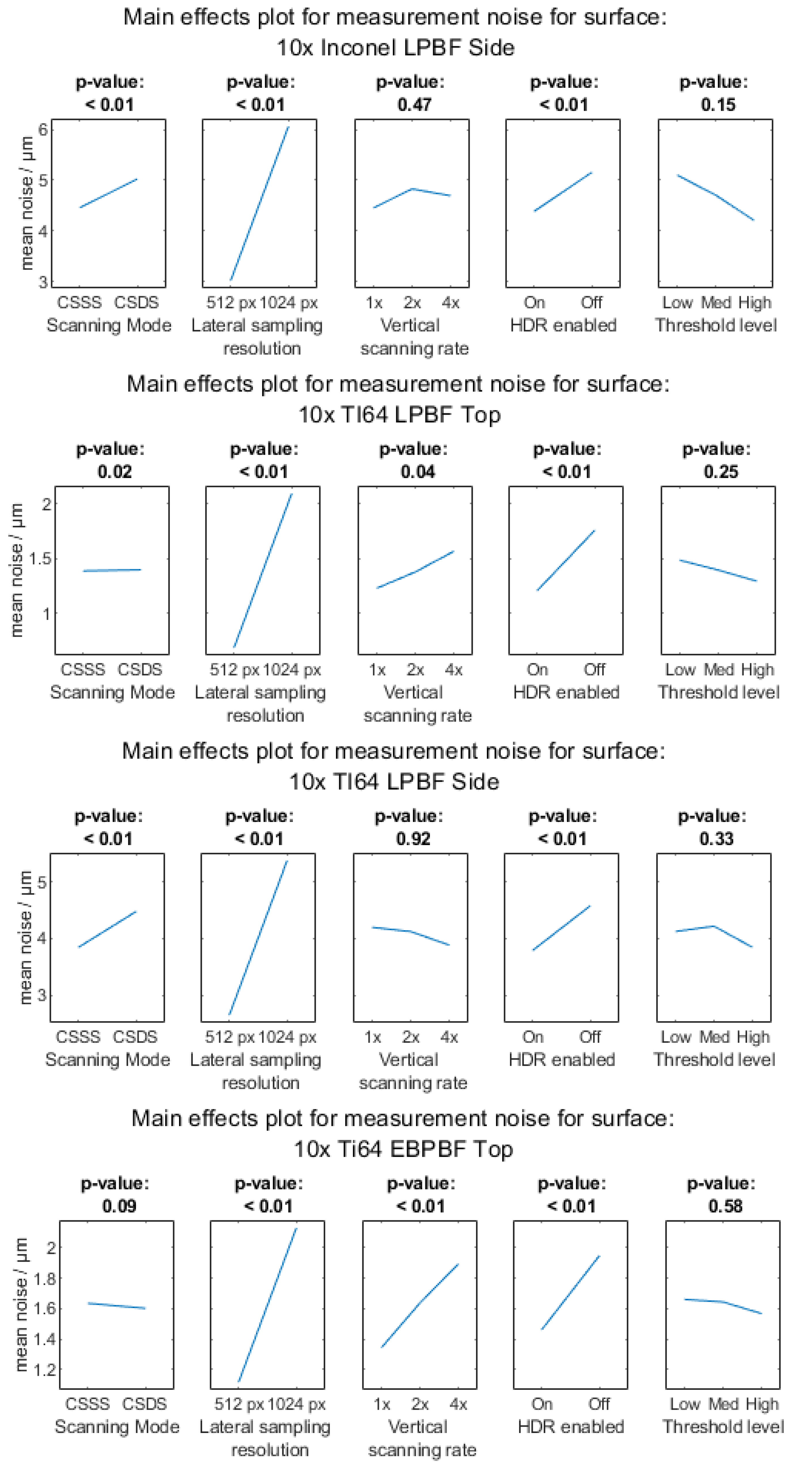
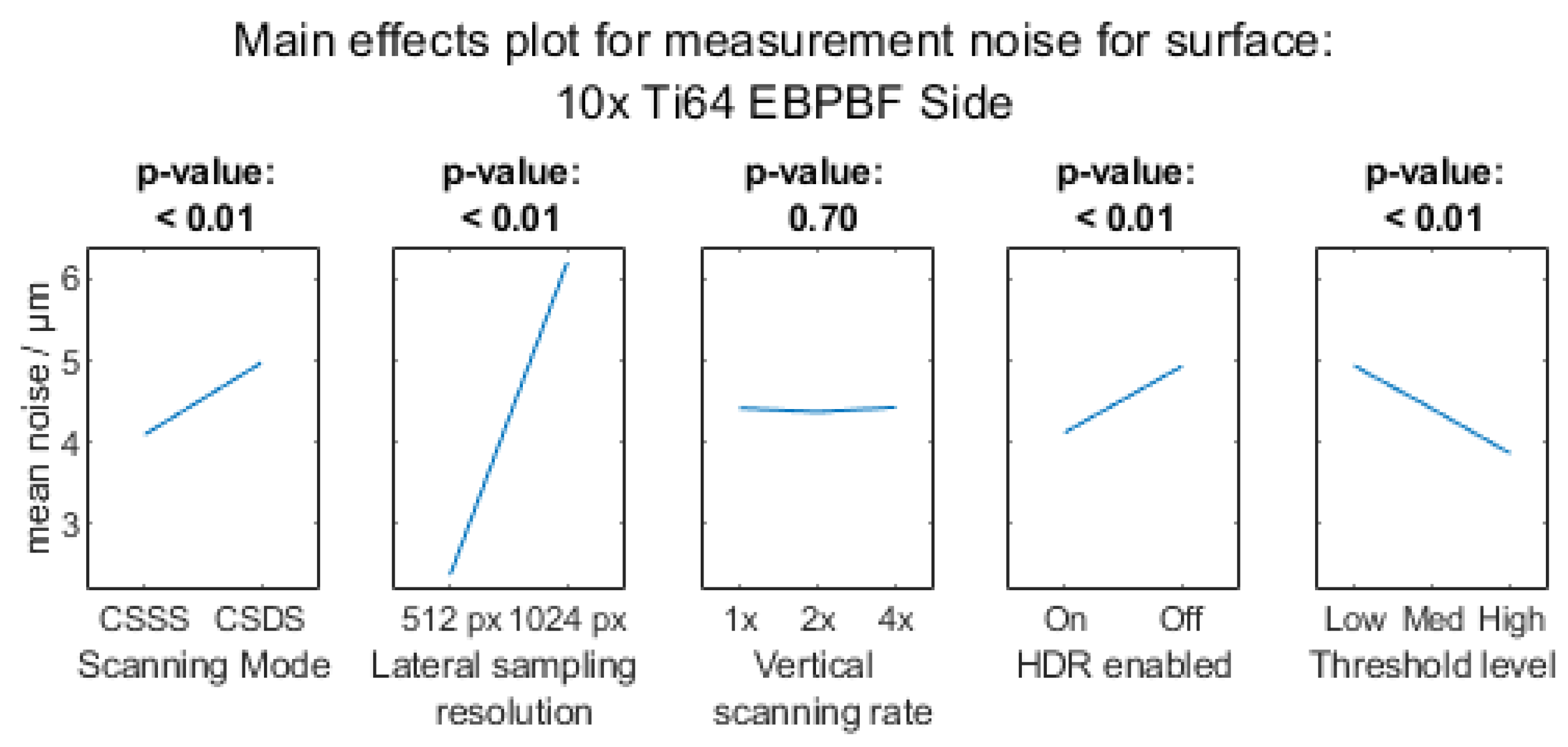
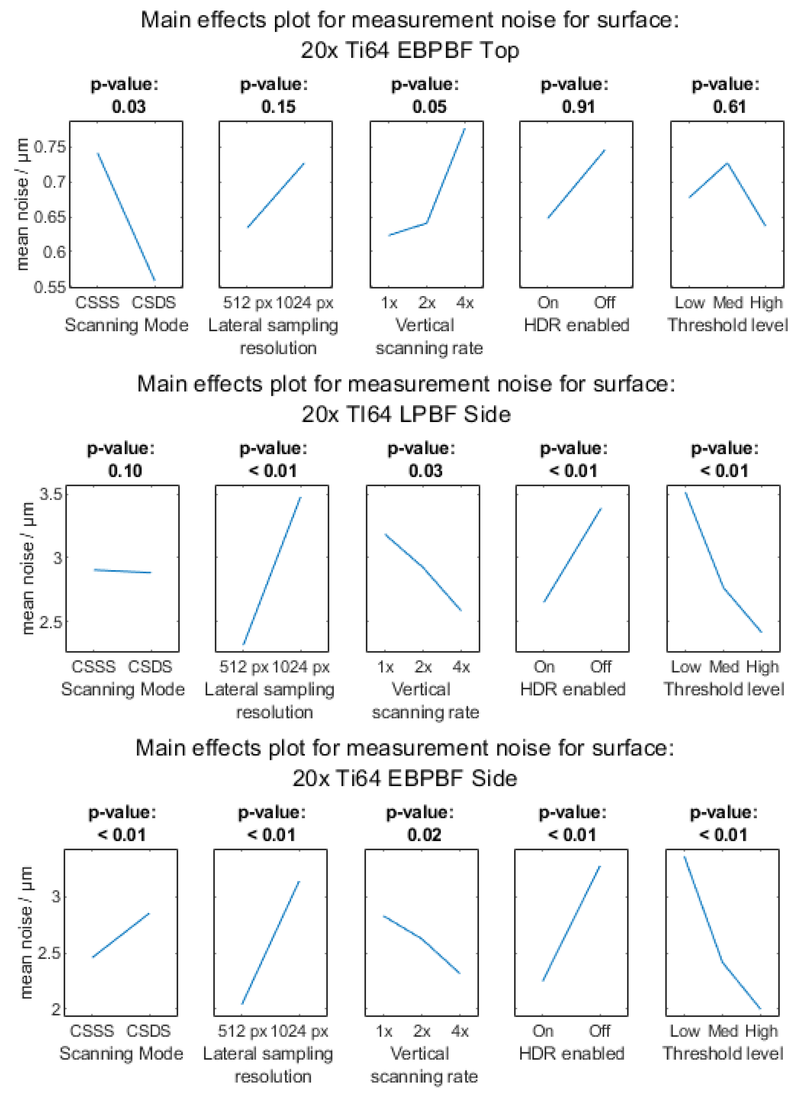
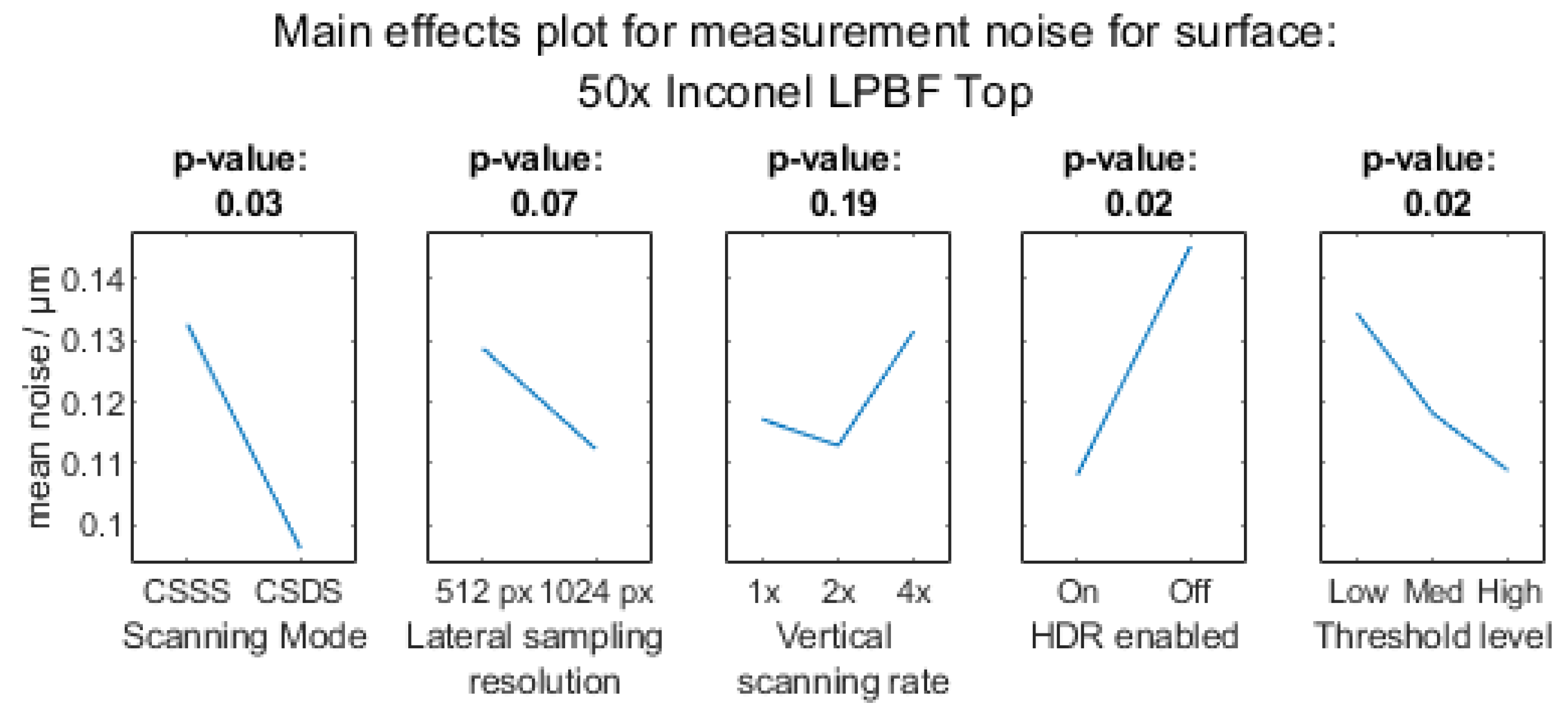
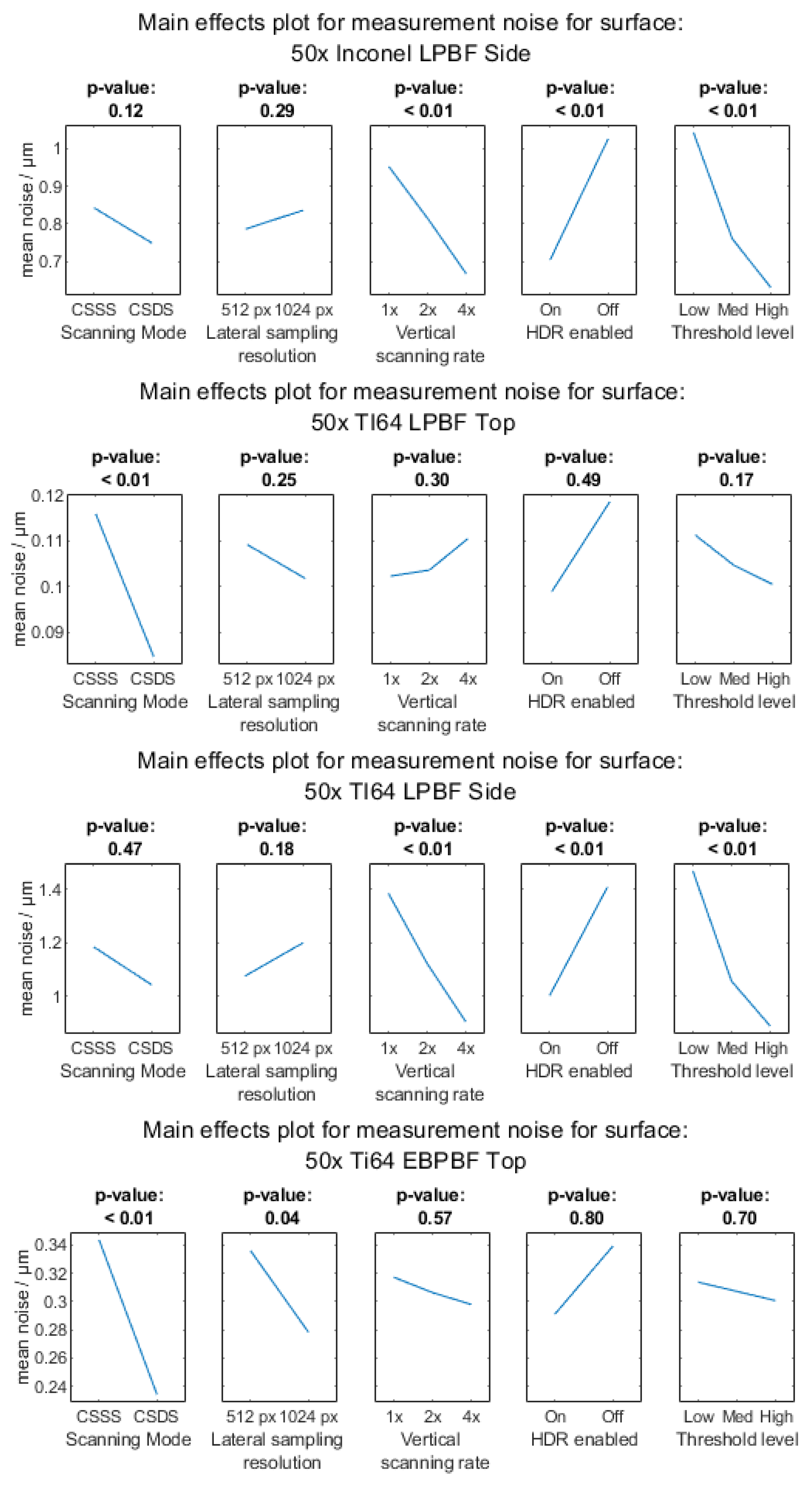
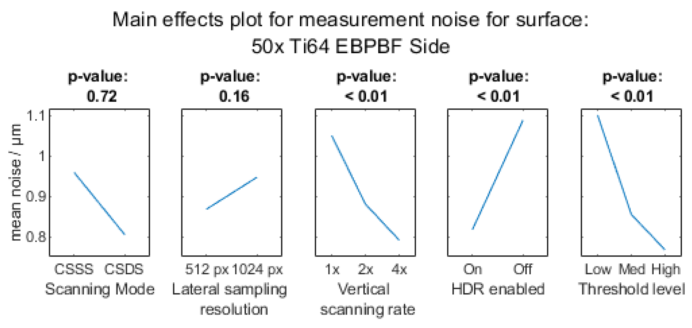
• Measurement noise (noise) was quantified using the subtraction method (see [28] for details). This is computed by considering the subtraction of two topographies, after a subtraction of the least-squares mean plane—a form-removal operator (ISO 25178-3 [29] F-operator)—for all combinations of the three measured repeats (taken in quick succession). This resultant height map should be dominated by the difference in the noise component between two repeat measurements. The noise can be estimated by the ISO 25178 part 2 [30] parameter Sq—the root-mean-square height of the resultant subtracted topography map divided by the square root of 2. The lower this value for the same measurement time and lateral resolution, the better.
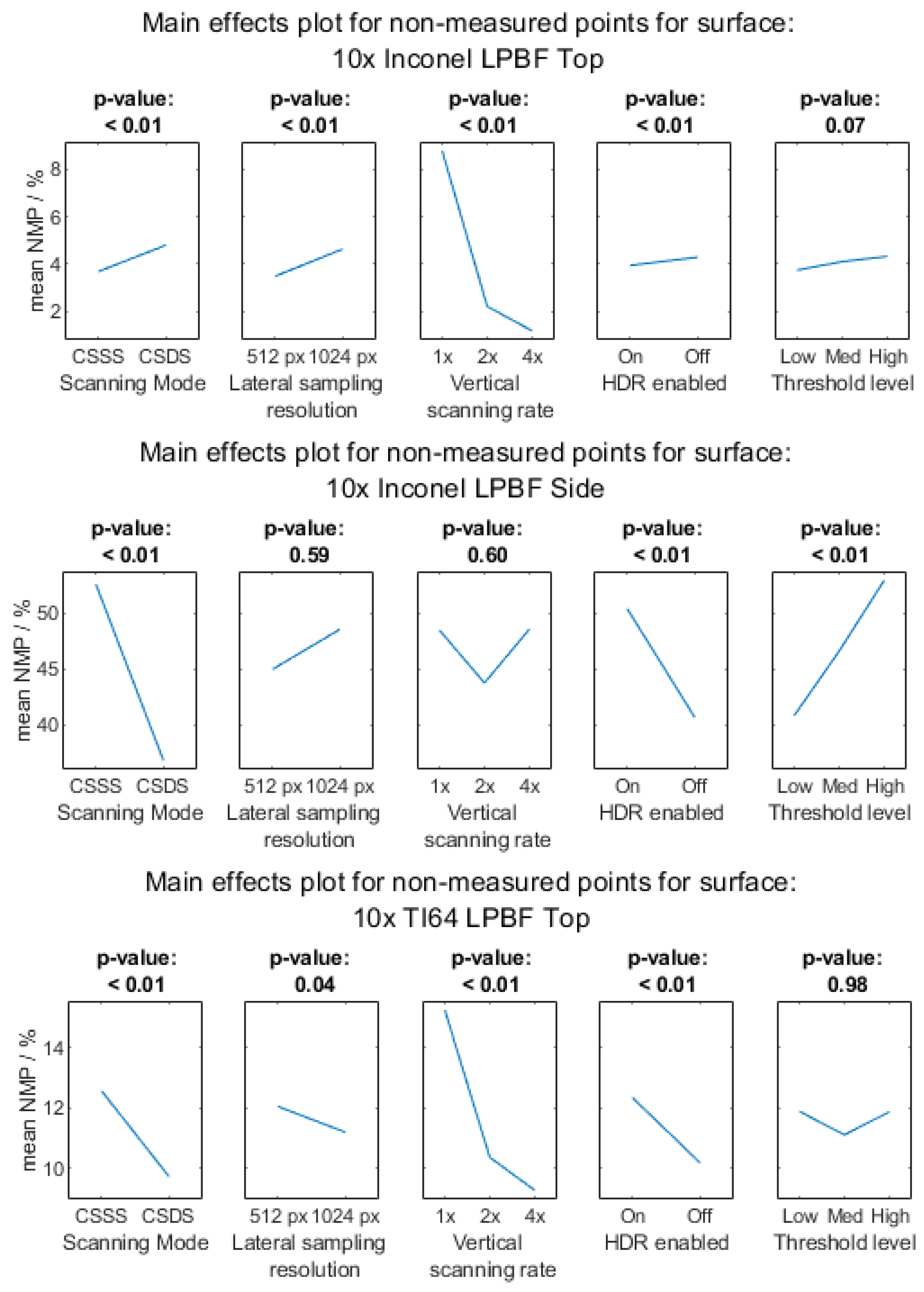
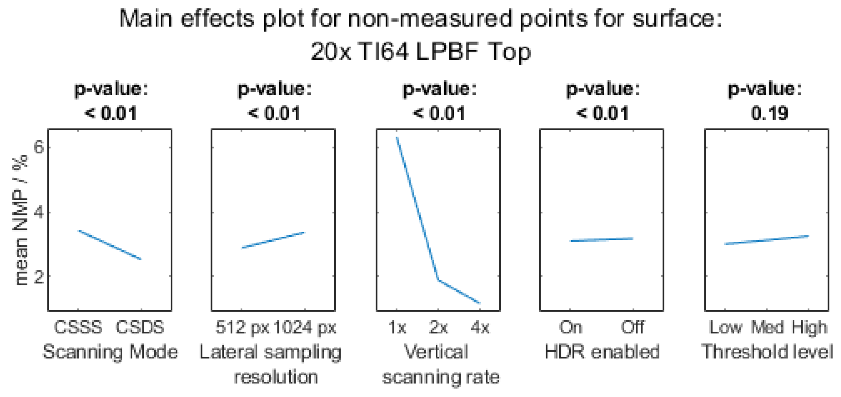
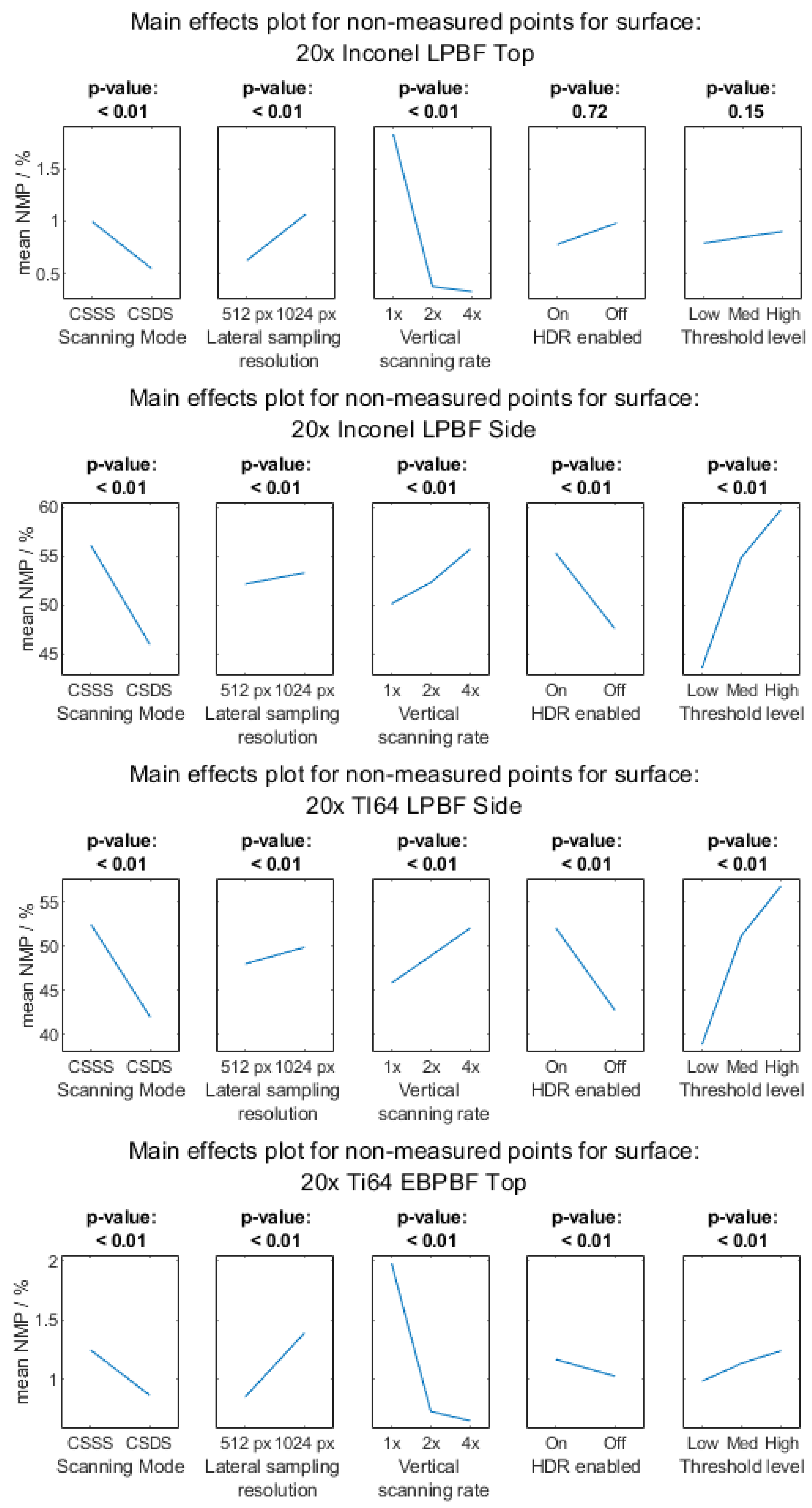
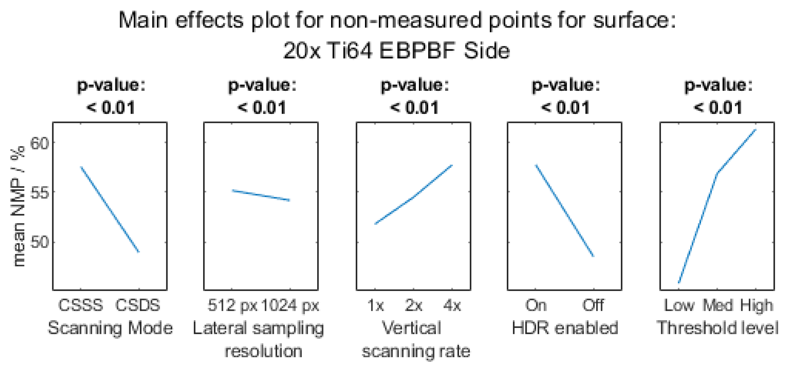
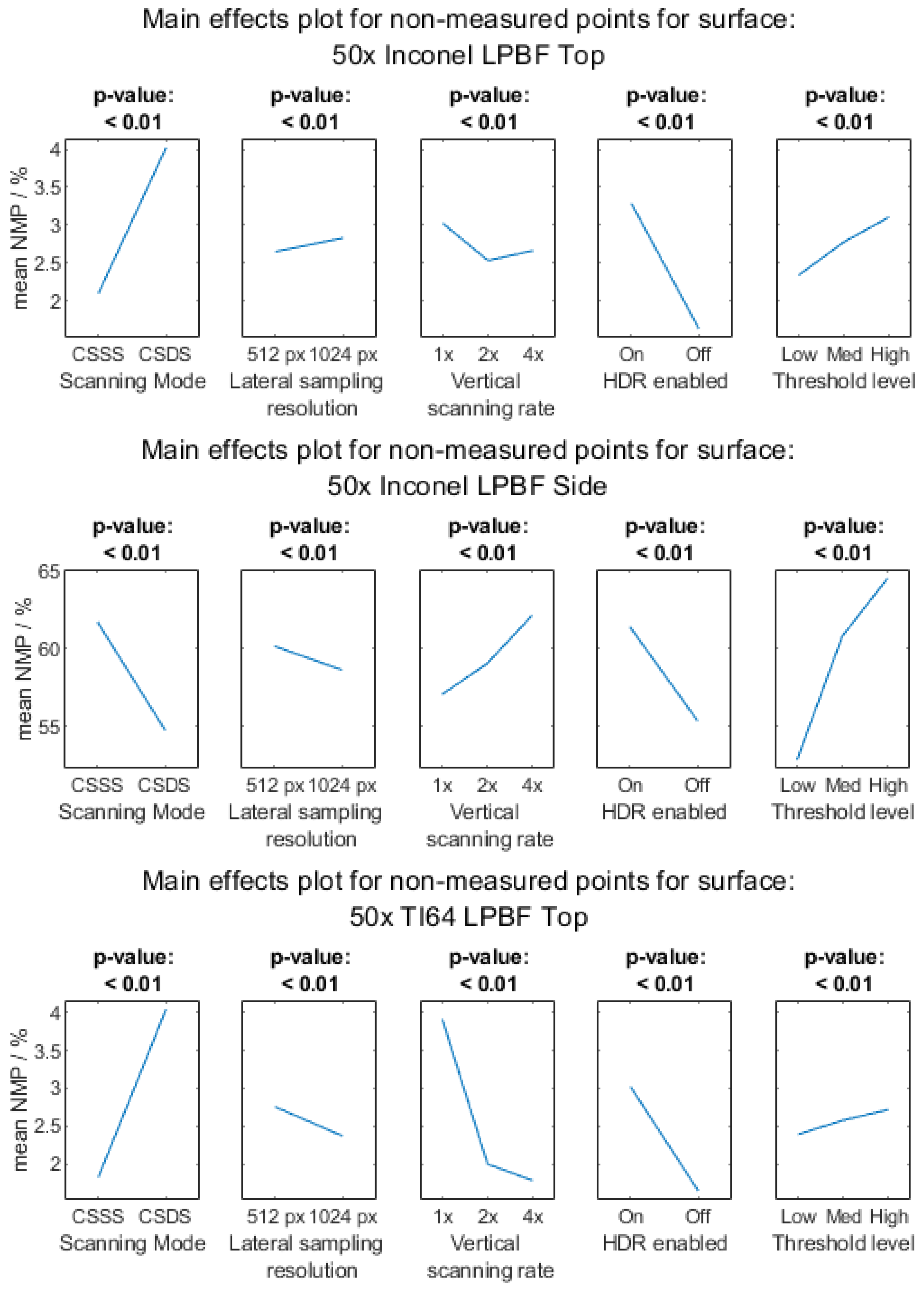
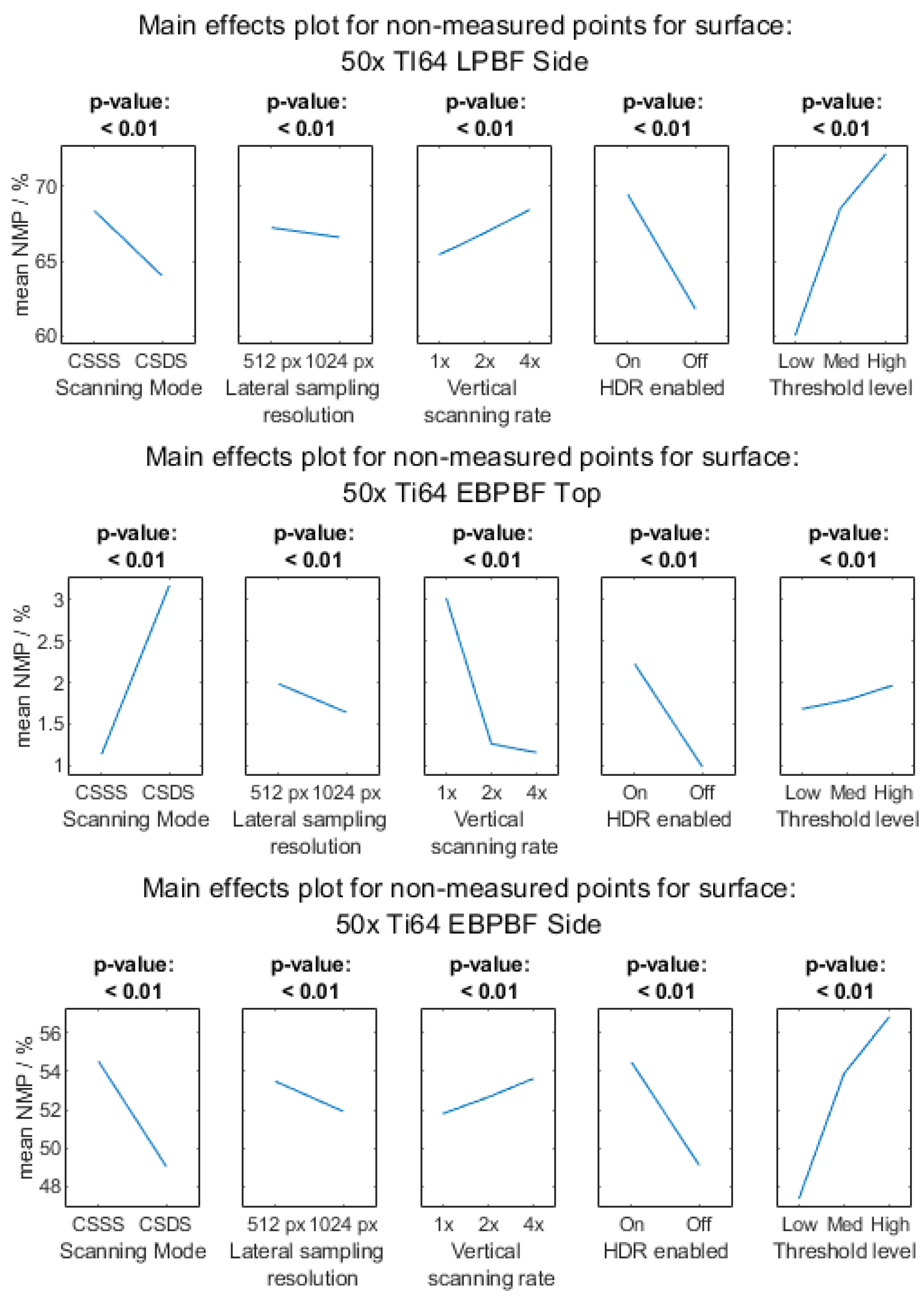
• Non-measured points (NMPs) were calculated as a percentage of the sum of NMPs over the total measured points of the surface topography within each height map. These are points for which the instrument does not acquire enough information, flagged by the instrument itself as non-measured. The lower this value, the better, provided no spikes appear and/or the noise is increased.
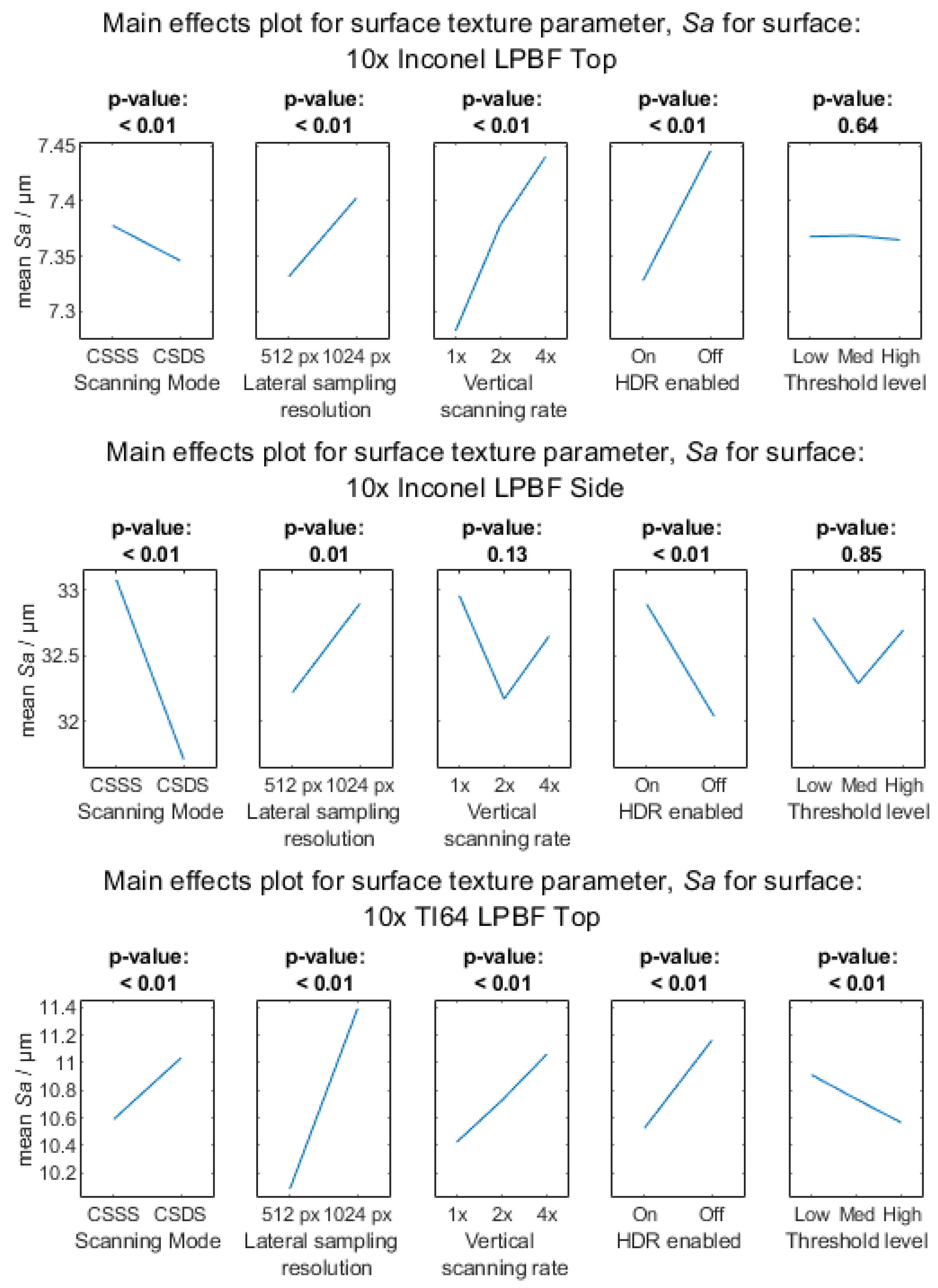
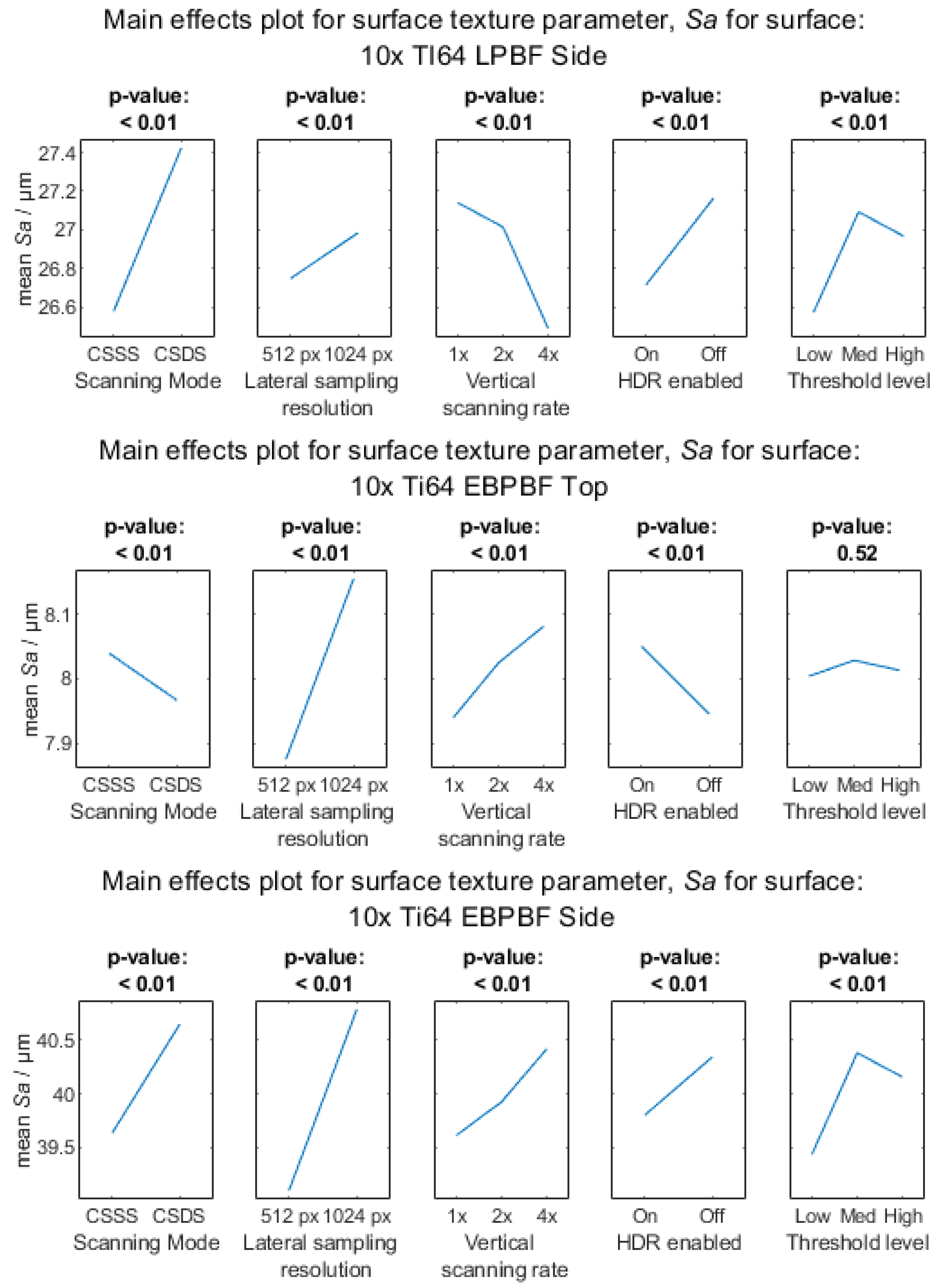
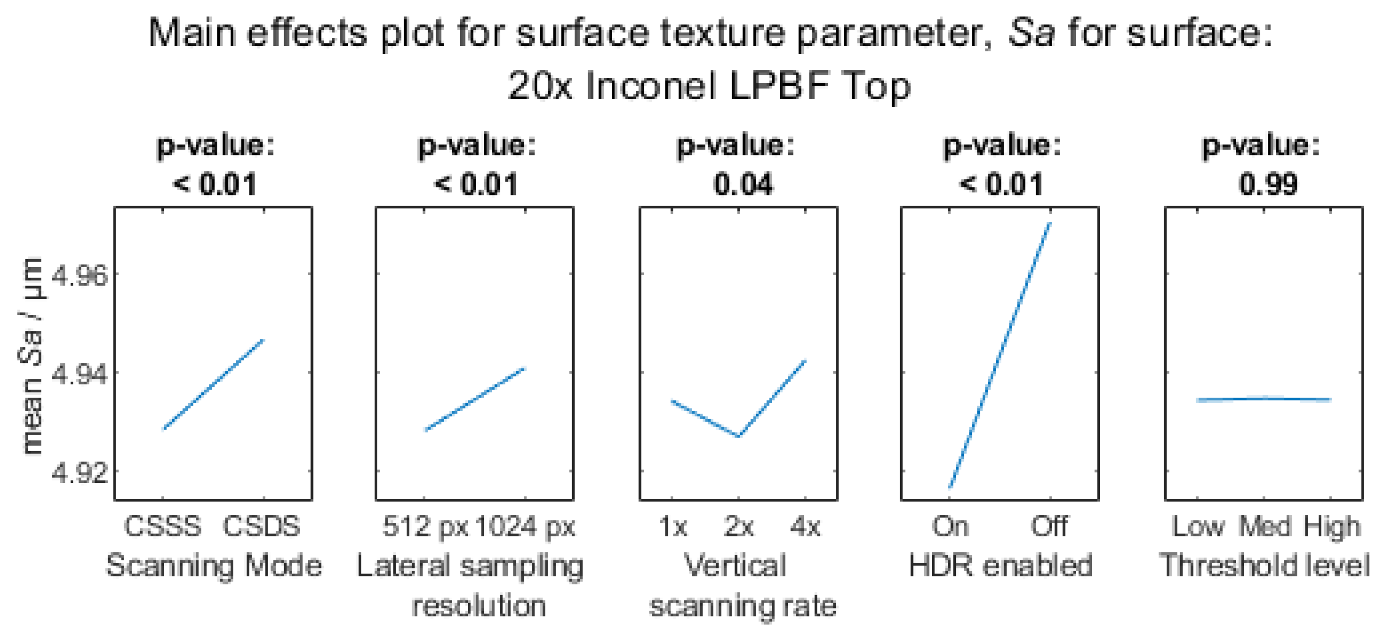
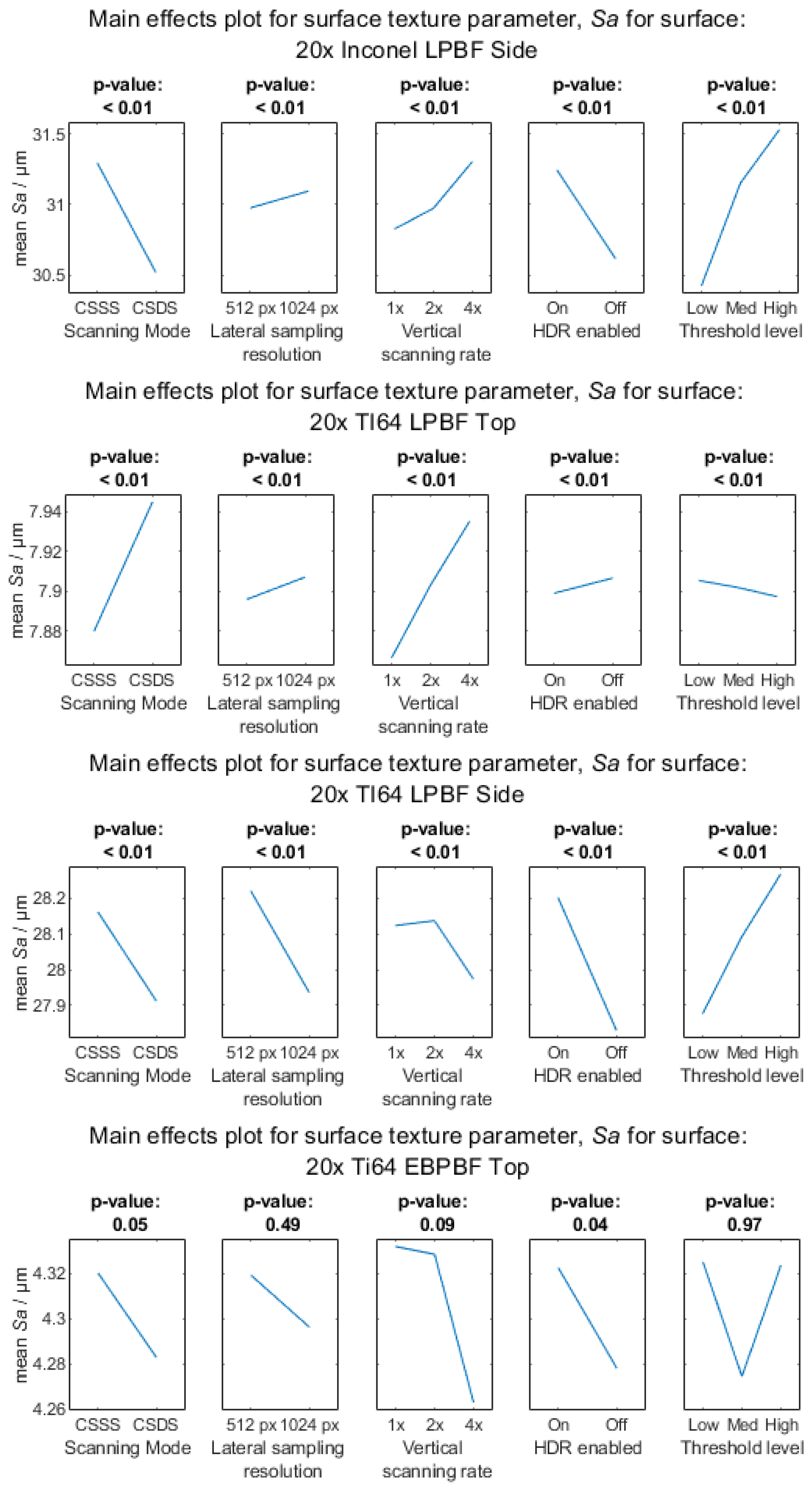
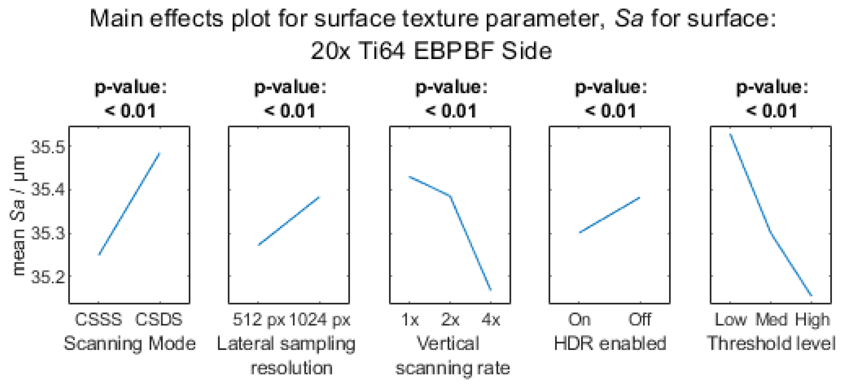
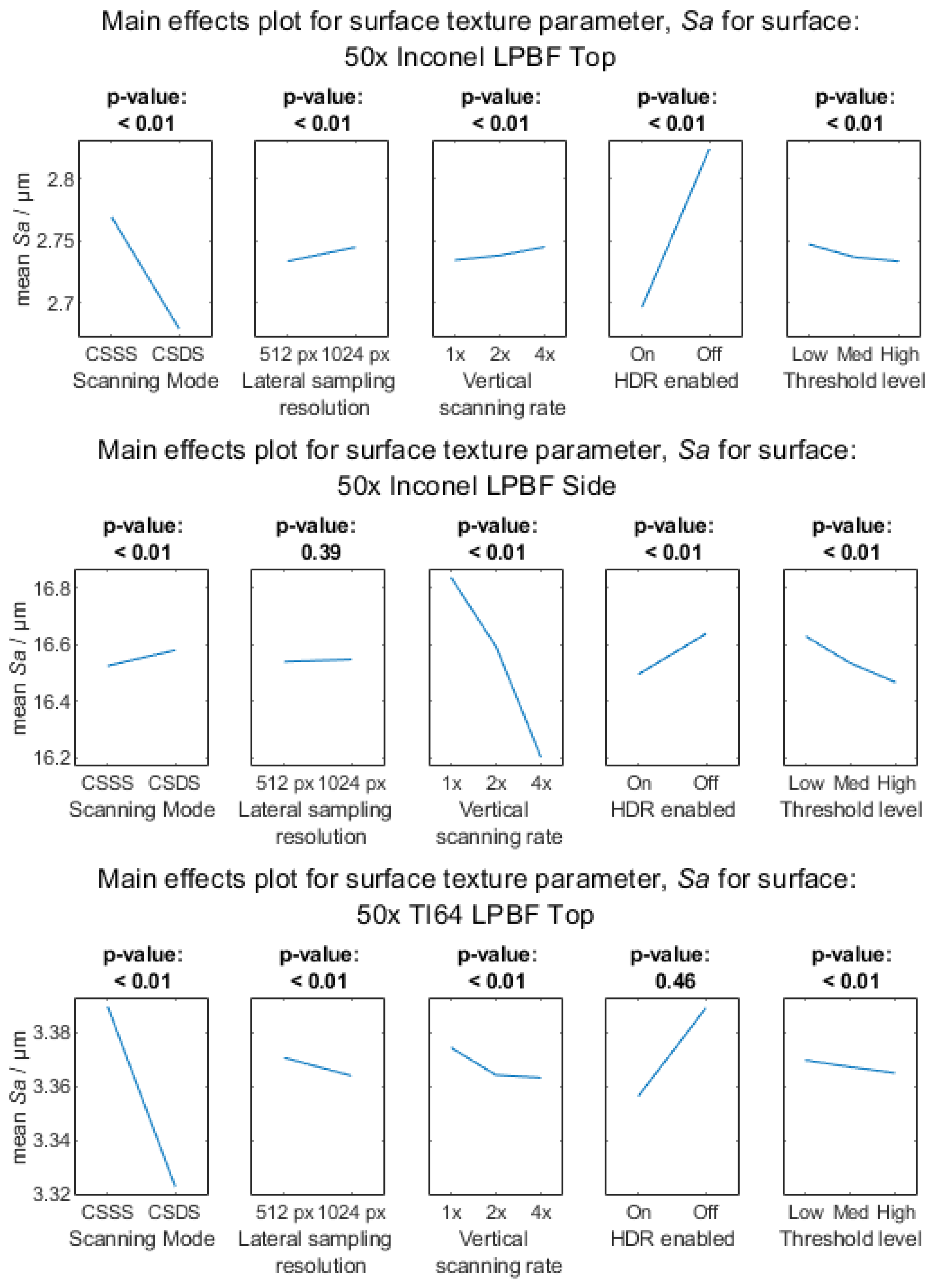
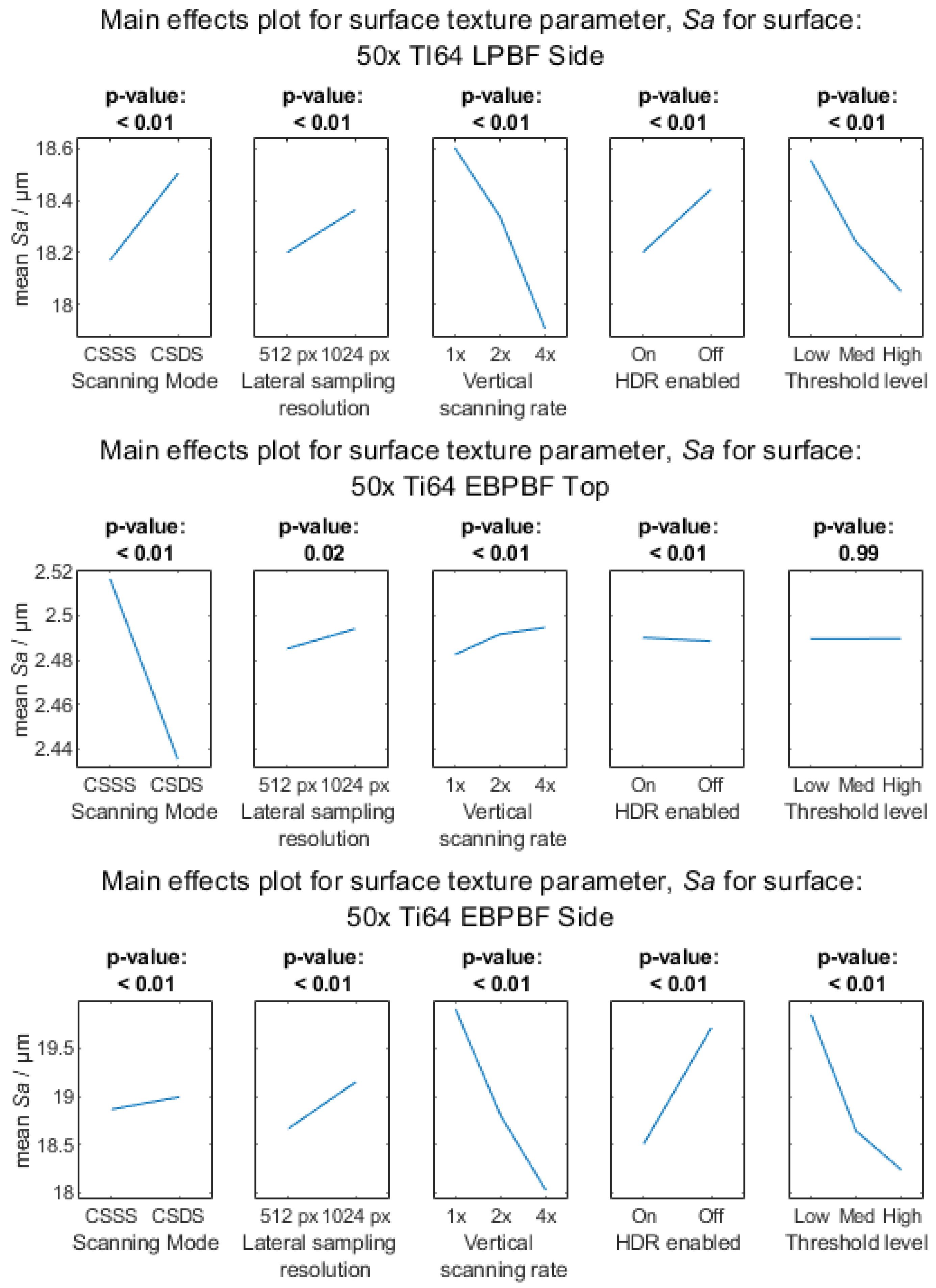
• The arithmetic mean height of the scale-limited surface Sa [30] was considered. To compute this parameter, only a least-squares mean plane by subtraction was used as a form-removal operator (ISO 25178-3 [29] F-operator). The parameter was computed with no further filtering applied (i.e., no separation of texture components at different spatial wavelengths), accepting the implicit operation of the lateral resolution and the NA of the objective as an S-filter [31].

MountainsMap 9 by Digital Surf [32] was used for visualisation, metric computation, processing of the topographies, and computation of the surface texture parameters.

2.5. Data Analysis

As in the work for FV [8], three independent full factorial designs of experiments (DOE) were produced for each performance metric (noise, NMPs, and Sa) for the six surface regions at each magnification. With the DOE, the sensitivity of these metrics to scanning mode, lateral sampling resolution, vertical scanning rate, HDR, and thresholding can be determined. Main effects plots and their statistical significance were investigated using analysis of variance (ANOVA) [33]. For each model, the coefficient of determination, R², was inspected to assess the fit of the model. Each independent variable has a reported p-value to indicate the significance to affect the result (using a p < 0.05 to indicate the likelihood that changes in the factor value reflect changes in the response variable).

Regarding NMP-filling operations, while relatively common in surface texture characterisation, these operations essentially make up information by nearest-neighbour interpolation or some other method. As our aim here was to study the interaction between the confocal microscope and the metal AM surface, we did not perform any such data-filling operations. Similarly, we did not perform any data-cleaning operations (for example, outlier removal) beyond any outlier removal inherently performed by the instrument manufacturer’s software.

3. Results

3.1. Comparison between Stylus Instruments

From the stylus results in Table 1 from [8], we can see that whilst the Ti-6Al-4V PPF-LB top surface is rough, most of its side surfaces possess a higher Ra value than their top surface counterpart. This might be explained by the stylus measuring particles/spatter or the thermally induced waviness found on this surface, which was not present on the top surfaces. Top surfaces are typically characterised by the presence of weld tracks and weld ripples, affected by the scanning strategy and any spatter that occurs, leaving some particles [4,34]. Side surfaces built by PBF are typically dominated by adhesion of the powder bed to these surfaces [5]. While areal and profile parameters cannot be meaningfully compared, the differences between them can be seen by comparing them to the results of

Table 2. ISO 21920 part 2 Ra parameter, for the test surfaces measured using a contact stylus instrument. Taken from [8].

Surface	Ra/μm
Inconel 718 PBF-LB top surface	6.2 ± 1.3
Inconel 718 PBF-LB side surface	18.7 ± 1.8
Ti-6Al-4V PBF-LB top surface	25.6 ± 3.2
Ti-6Al-4V PBF-LB side surface	19.7 ± 2.9
Ti-6Al-4V PBF-EB top surface	6.7 ± 1.8
Ti-6Al-4V PBF-EB side surface	26.8 ± 3.2

(in [8]). Table 2 shows the mean and standard deviation of the areal surface texture parameter Ra, which can be compared to the mean values on the main effects plots for the surface texture parameter Sa for the 10× objective (all main effects plots of the surface texture parameter can be found in the Appendix A). Whilst the profile and areal parameters differ, which can be explained by the differences between FoV and sampling, only the trend for the Ti-6Al-4V PBF-LB surfaces differs, where the top surface has a lower Sa result than the side surface.

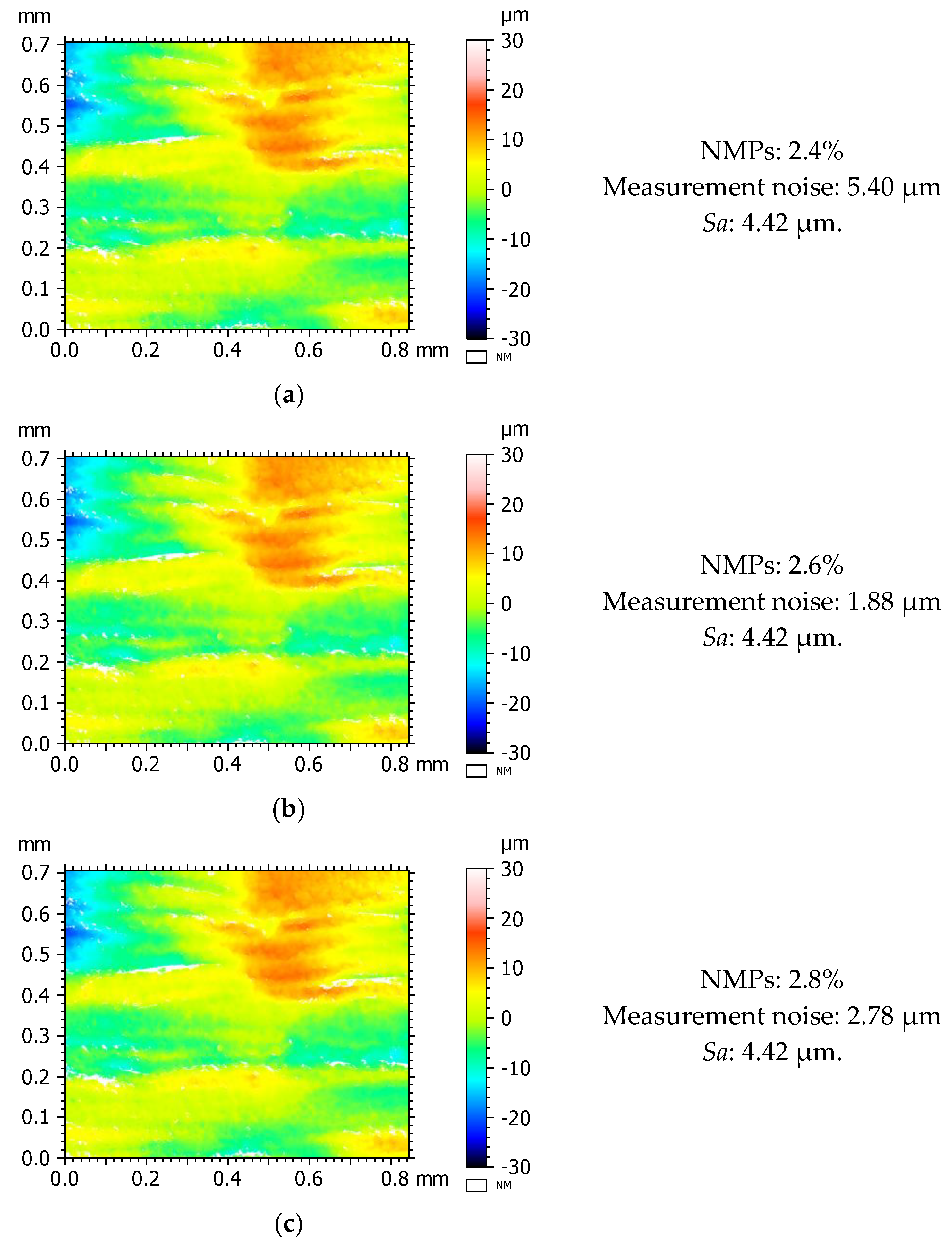
3.2. Visualisation of the Influence of Measurement Parameters

Height maps for the topographies of the various surfaces are shown in Figure 4, Figure 5, Figure 6, Figure 7, Figure 8 and Figure 9. These height maps show some of the challenges presented to the CM when overcoming deep recesses and particle structures on the surfaces. There is the presence of features with high local slopes and/or high aspect ratios, presenting challenges for the measurement. The topographies appear to vary significantly between the process and orientation, creating an obstacle to finding a singular optimised measurement setup for all surfaces.

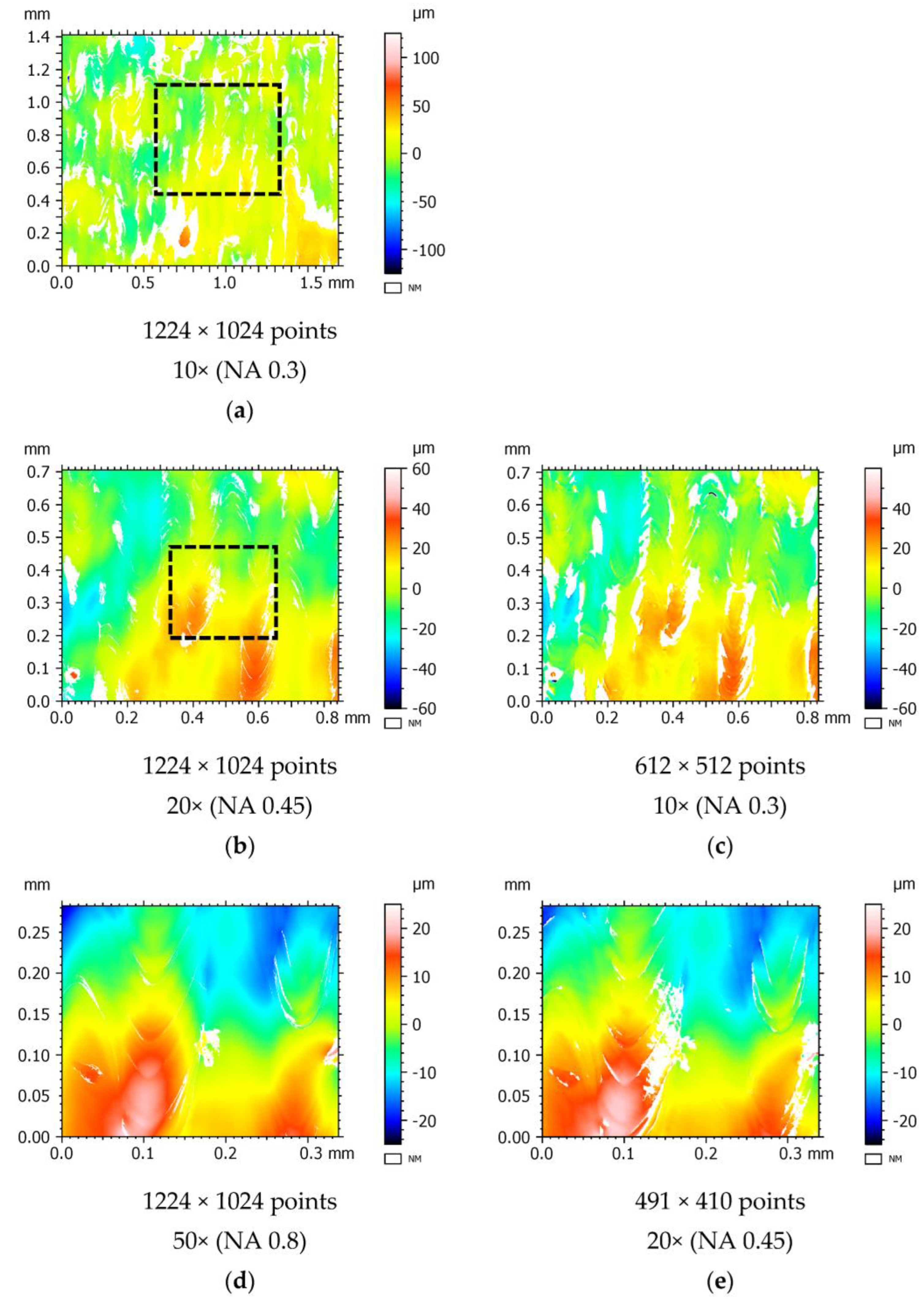
3.2.1. Effect of Changing Magnification on Surface Topography Measurement

The choice of magnification depends on the goals of the measurement. Different objectives can be chosen to better enable measurement of different surface features captured in the measurement and to achieve a different lateral resolution because of the combination of pixel size and NA. However, higher magnification (which often has higher NA and improved lateral resolution) will have a smaller field of view, which can make the measurement of large areas through stitching excessively long. Figure 4 shows the Ti-6Al-4V PBF-LB top surface topography at increasing objective magnifications. At the lowest magnification, there are clear patterns of weld tracks and an underlying waviness component (due to thermal effects), while at higher magnifications, small-scale features such as weld ripples become more prominent.

3.2.2. Effect of Changing Scanning Mode on Surface Topography Measurement

Height maps showing the same Ti-6Al-4V PBF-LB side surface obtained with different scanning mode settings are shown in Figure 5. Changing the CSSS setting to the CSDS setting increases the measurement time, as the system must scan in two directions for each confocal image. This increased sampling for each confocal image may help the instrument in capturing difficult-to-measure regions, such as the edges of particles and recessed surface regions. The improvement from 82.6% NMPs to 21.1% NMPs is representative of the large and significant improvements with the use of CSDS for side surfaces. There is not such a significant improvement visible for top surfaces, as the CSSS setting often results in a small number of NMPs.

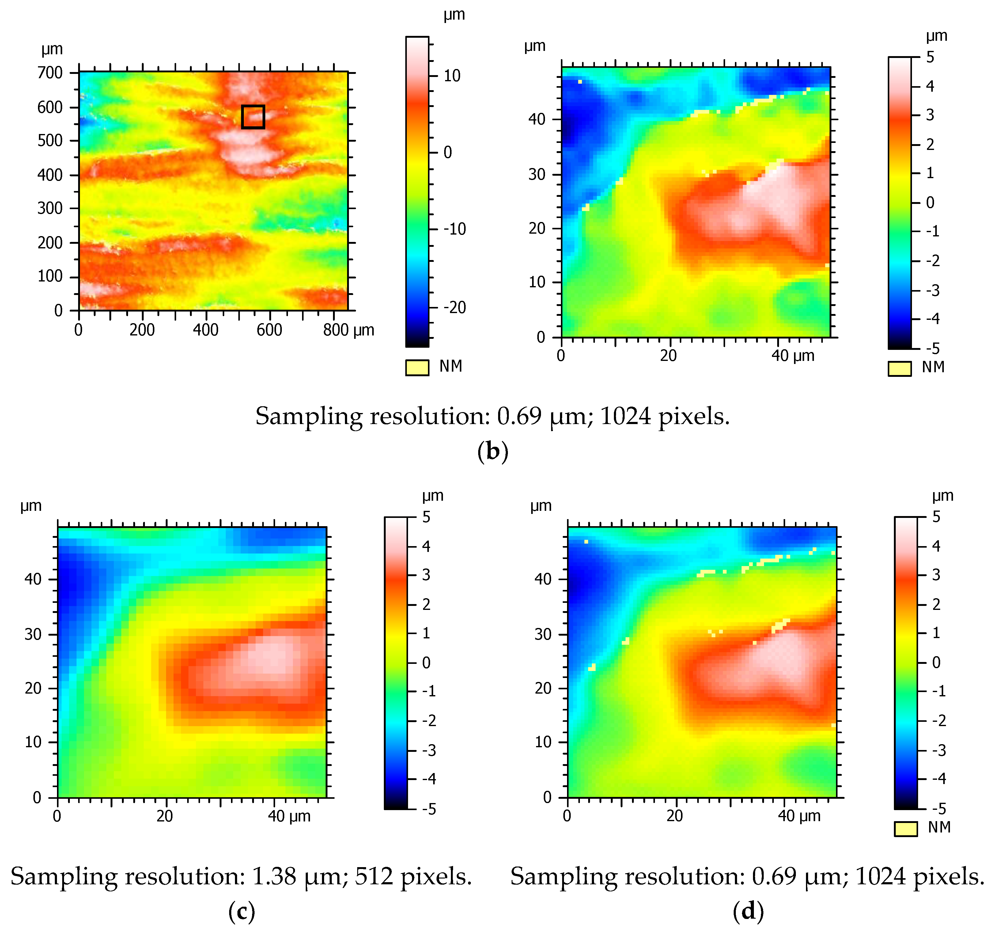
3.2.3. Effect of Changing Lateral Sampling Resolution on Surface Topography Measurement

The effect of the lateral sampling resolution on measurement is visualised in Figure 6. While on the full topography there is no clear difference, there is an expected reduction in resolution between the higher and the lower resolution. This reduction in lateral sampling resolution can cause a smoothing effect to occur, as lower numbers of pixels are being used over the same measurement area. This setting might be used when considering stitching of images to measure a larger measurement area in order to reduce the file size of the measurement data, but it should be considered against whether there are small-scale features that might be filtered out by this downsampling. Moreover, the lateral resolution limitation from the objective should be considered; if this resolution is larger than the pixel size, the system/signal noise can be decreased by taking a larger sampling resolution, without affecting the topography noise. The same can be achieved by applying an S-filter [31]—an effect that can be seen in Figure 6c,d.

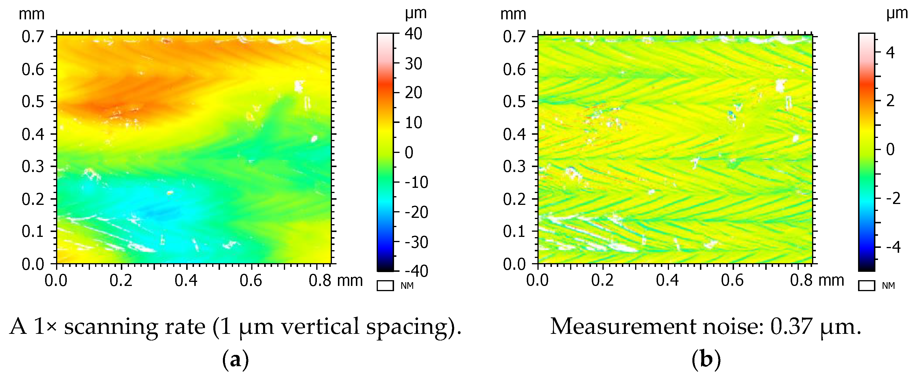
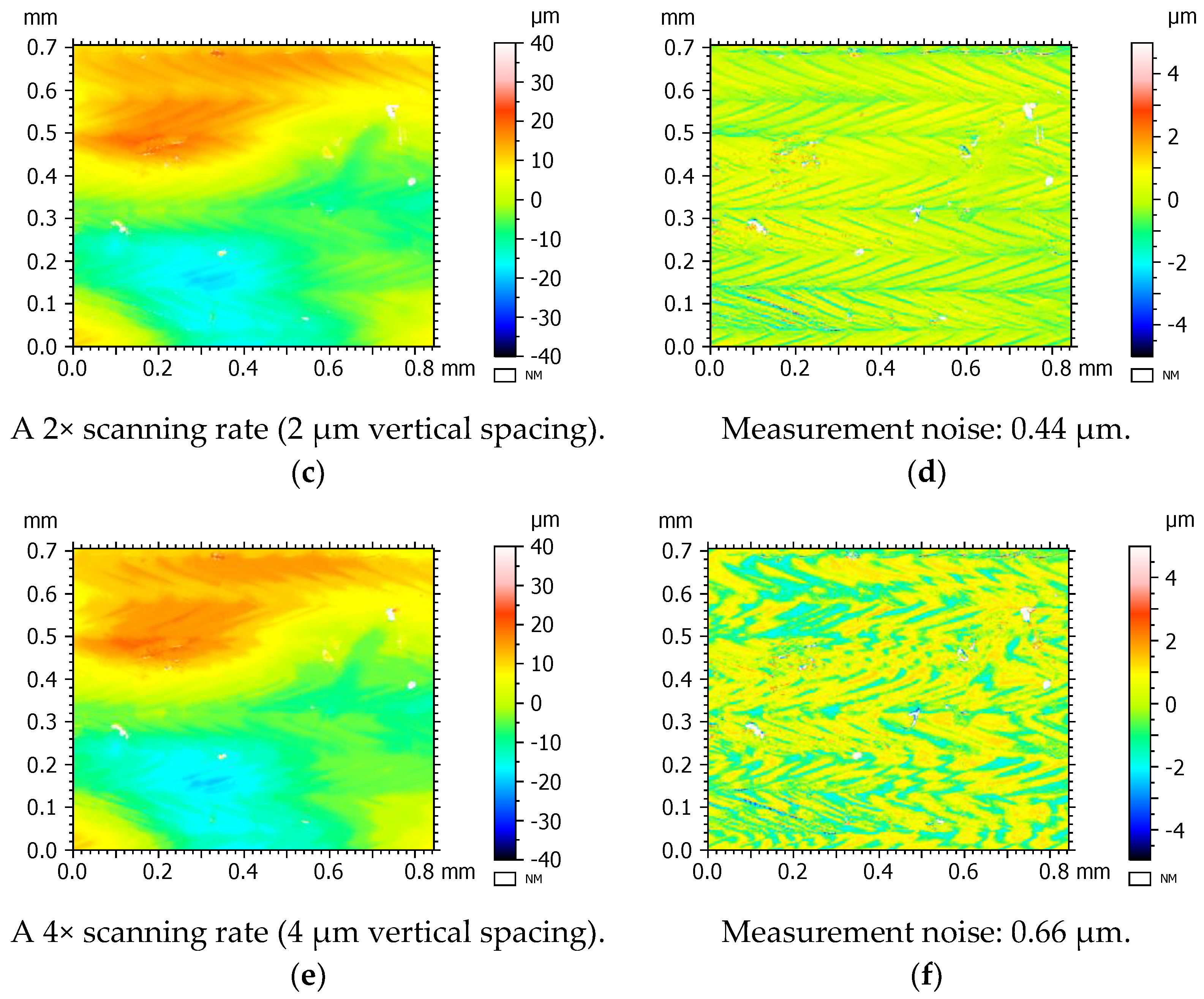
3.2.4. Effect of Changing Vertical Scanning Rate on Surface Topography Measurement

Height maps measured with different vertical scanning rates can be seen in Figure 7. With fewer confocal images taken in a vertical scan, higher scanning rates will significantly reduce the measurement time but lead to increased noise. The reason for increased noise is that higher scanning rates will sample fewer confocal images over the same measurement range. This reduced sampling of confocal images will increase the reliance on interpolation between confocal images to determine the vertical position of maximum intensity, which represents the height point. A faster, higher scanning rate may be useful for stitching a large number of FoVs into a larger measurement result to account for the total measurement time, but this must be balanced against any loss in measurement repeatability and increase in noise. Based on visual inspection, there is some small reduction in NMPs with a higher scanning rate, but few noticeable differences between the topographies. Across the difference maps, there are larger discrepancies on the edges of the weld ripples, consistent across all scanning rates, suggesting that these regions of local curvature are regions where noise is higher. For the noise itself, there is a proportional increase with increased vertical scanning rate, suggesting that with larger spacing between confocal images there is potential for higher error in the determination of points on the surface (which would be expected).

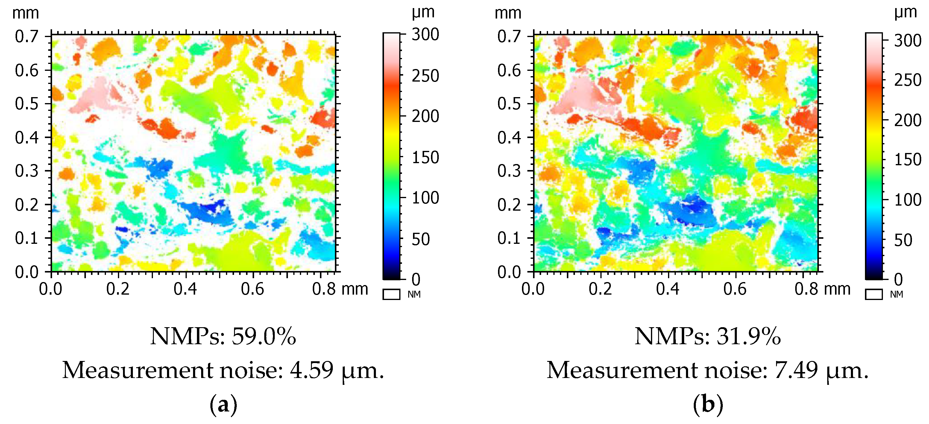
3.2.5. Effect of HDR on Surface Topography Measurement

The HDR setting would be expected to add to the total measurement time when enabled, as multiple scans are taken with differing illumination intensities for a single measurement. These repeats with differing illumination intensities act to overcome issues with varying reflectivity or deep recesses over the FoV to capture the optimal measured points, as shown in Figure 8 for the same example surface measured with only the HDR setting changed. When HDR is enabled, there are more NMPs present in the surface height map, but with less small-scale height variations when comparing the regions of measured points. Meanwhile, contrary to expectations, the HDR setting involves some algorithmic threshold to determine which point from the repeated measurements to use, and it will not determine a point if none of the repeated measurements’ height points fall within this threshold. Use of the HDR setting results in measurements with higher numbers of NMPs but lower overall noise for all measured points when compared to not using the setting.

3.2.6. Effect of Threshold Level on Surface Topography Measurement

Height maps obtained at different threshold levels on the same surface can be seen in Figure 9. The threshold level setting would be expected to remove noisy data points and replace them with NMPs; this explains the reduction in noise and increase in NMPs between the lower and higher threshold levels. In terms of visual inspection, changes in threshold level produce few appreciable topographic differences. As shown in the figure, the Sa parameter is not influenced significantly by the threshold level, but the number of NMPs does increase with increasing threshold, showing the effect of thresholding on removing points in the measurement. For this example, there is a reduction in noise between the low- and high-level settings, but this is not consistent for all level changes (see the figures in Appendix A).

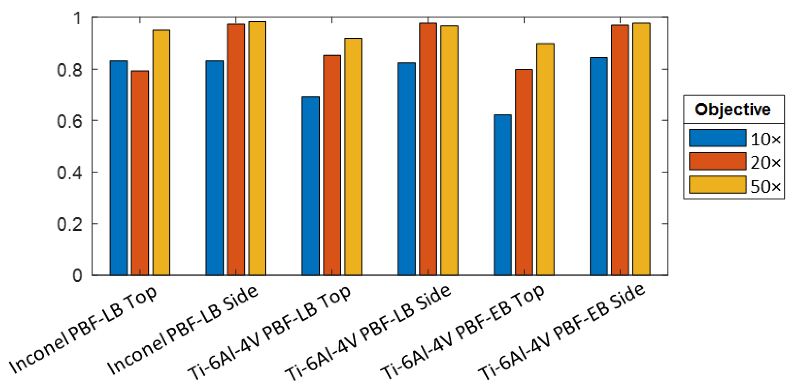
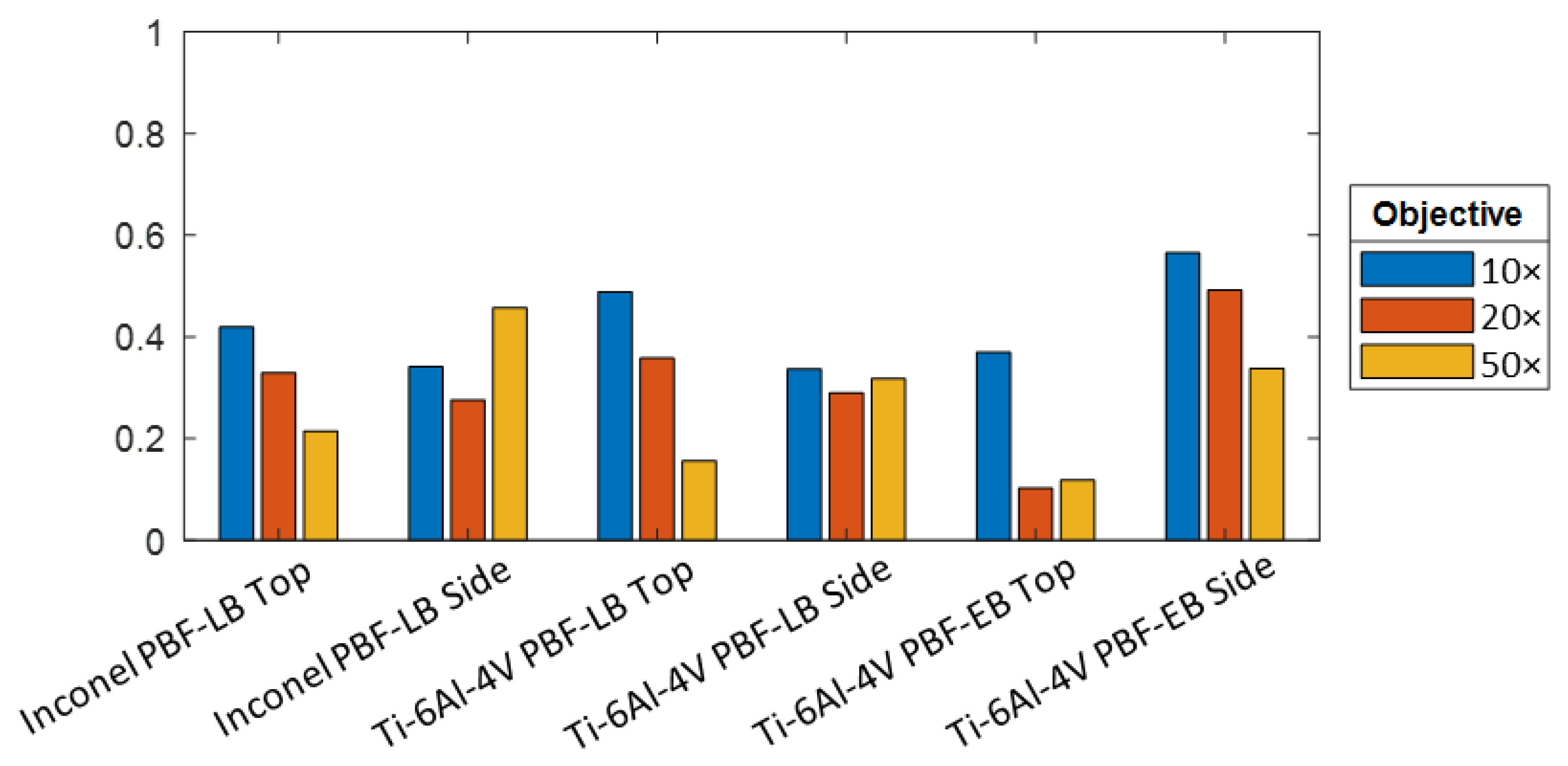
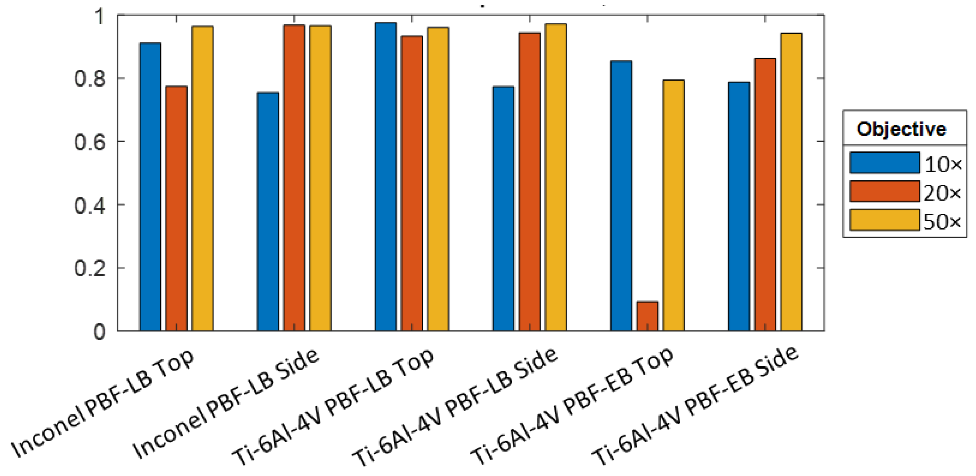
3.3. Coefficient of Determination for Linear Models

In Figure 10, Figure 11 and Figure 12, the coefficient of determination for the linear models is plotted for all metrics, surface types, and objective magnifications. This coefficient will only represent the fitting between the statistical model, its predicted results, and the experimental results; it is this model that was later used to determine the significance of factors (i.e., measurement process parameters) through ANOVA [33]. Figure 10 shows the R² for models for the number of NMPs, with most of the results for higher objective magnifications showing a good fit with the model (i.e., R² close to or greater than 0.8). The 10× objective shows weaker fits for all models, with the weakest fits found for the PBF-LB top surfaces. All models show weaker relative fits to the model for top surfaces than for side surfaces.

For the noise, there are significantly low values for fitting, as shown in Figure 11. These low values indicate that the relationship between the predictions from the linear model and the experimental results is weak. This poor fitting may be due to a weak linear relationship between these parameters and noise, and it is not an ideal type of model for these data—the relationship may in fact be nonlinear. While the R² is low for this metric, this does not diminish the significance of any factor or any main effects plots that can be used to observe the influence of the measurement process parameters on the noise.

For the surface texture parameter Sa (see Figure 12), the R² coefficients show a good fit for most models. Most of the goodness-of-fit values are above 0.7, showing relatively good fitting, but only the Ti-6Al-4V PBF-EB top surface specifically measured using the 20× objective shows poor fitting. The goodness-of-fit values suggest that the significance of the ANOVA [33] for these models should be a valid assessment, with the exception of the Ti-6Al-4V PBF-EB top surface, where only the large main effects should be considered. For the Ti-6Al-4V PBF-EB top surface, validation is required by comparing these significances against the main effects plots.

3.4. Summary Tables for Main Effects Plots of Measurement Process Parameters

Using ANOVA [33] on the linear models for each surface type and objective magnification, the significance of each measurement process parameter was calculated; these are shown alongside the main effects plots, which are reported in full in Appendix A. To simplify the analysis of the relationships between each metric (i.e., number of NMPs, noise, Sa) and the measurement process parameters, only the largest and/or most significant main effects are summarised within

Table 3. The main effects for all measurement process parameters with non-measured points. The information within is derived from Figure A1, Figure A2, Figure A3, Figure A4, Figure A5, Figure A6, Figure A7, Figure A8 and Figure A9 in Appendix A. Summaries are grouped by magnification and surface orientation. The summary refers to the size of the effect, which refers to the distance between the means at the two simplified levels (with small representing close means and large representing more distant means), and correlation with respect to the factors (positive or negative). An empty field indicates that no main effects trend is consistent or significant for all surface groupings.

Magnification	Surface Orientation	Scanning Mode		Lateral Sampling Resolution		Vertical Scanning Rate		HDR Enabled		Threshold Level
		CSSS	CSDS	Low	High	Low	High	On	Off	Low	High
10×	Top	Large negative		Small negative		Large negative		Small negative		-
	Side	Large negative		Small negative		-		Large negative		Large positive
20×	Top	Small negative		Small positive		Large negative		-		-
	Side	Large negative		Small negative		Large positive		Large negative		Large positive
50×	Top	Small Positive		Small negative		Large negative		Large negative		Small positive
	Side	Large Negative		Small negative		Small positive		Large negative		Large positive

,

Table 4. The main effects for all measurement process parameters with noise. The information within is derived from Figure A1, Figure A2, Figure A3, Figure A4, Figure A5, Figure A6, Figure A7, Figure A8 and Figure A9 in Appendix A. Summaries are grouped by magnification and surface orientation. The summary refers to the size of the effect, which refers to the distance between the means at the two simplified levels (with small representing close means and large representing more distant means), and correlation with respect to the factors (positive or negative). An empty field indicates that no main effects trend is consistent or significant for all surface groupings.

Magnification	Surface Orientation	Scanning Mode		Lateral Sampling Resolution		Vertical Scanning Rate		HDR Enabled		Threshold Level
		CSSS	CSDS	Low	High	Low	High	On	Off	Low	High
10×	Top	-		Large positive		Large positive		Large positive		-
	Side	Small positive		Large positive		-		Small positive		-
20×	Top	-		-		Positive		-		-
	Side	-		Large positive		-		Large positive		Large negative
50×	Top	Negative		-		-		-		-
	Side	-		-		Large negative		Large positive		Large negative

and

Table 5. The main effects for all measurement process parameters with the surface texture parameter Sa. The information within is derived from Figure A1, Figure A2, Figure A3, Figure A4, Figure A5, Figure A6, Figure A7, Figure A8 and Figure A9 in Appendix A. Summaries are grouped by magnification and surface orientation. The summary refers to the size of the effect, which refers to the distance between the means at the two simplified levels (with small representing close means and large representing more distant means), and correlation with respect to the factors (positive or negative). An empty field indicates that no main effects trend is consistent or significant for all surface groupings.

Magnification	Surface Orientation	Scanning Mode		Lateral Sampling Resolution		Vertical Scanning Rate		HDR Enabled		Threshold Level
		CSSS	CSDS	Low	High	Low	High	On	Off	Low	High
10×	Top	Small negative		Large positive		Large positive		Small negative		-
	Side	Large negative		Small positive		-		Small negative		-
20×	Top	-		-		-		Negative		-
	Side	Large negative		Large negative		Small negative		Large negative		Large positive
50×	Top	Large negative		Small positive		Small positive		-		-
	Side	Small positive		Large negative		-		Small positive		Small negative

, and only for consistent trends. The summaries of the main effects are split by surface orientation and objective magnification. The terms “small” and “large” represent whether the group means are close (small effect) or far (large effect) from one another, respectively. The positive and negative refer to the orientation of the main effect.

Table 3 summarises the main effects plots for the number of NMPs found in Appendix A, describing only measurement process parameters that are significant factors within the groupings for surface orientation and objective magnification. For the scanning mode (apart from the 50× top surface), the main effects have a negative relationship. This result means that the CSDS scanning mode (which increases sampling on the confocal image) offers a consistent reduction in the number of NMPs, which is often one of the larger effects across all factors and surfaces. This increased sampling on the confocal images reduces the need for any internal thresholding to remove points on the surface. The averaging effect of the double sampling on the confocal image reduces noise in the measurement—which, in turn, reduces the need to threshold points in the measurement. There is always a small relative improvement when increasing the lateral sampling resolution, due to increased sampling raising the proportion of valid points that might otherwise be removed algorithmically.

There is a large, negatively correlated effect for top surfaces for vertical scanning rate (i.e., decreasing NMPs for increasing vertical scanning rate), showing that the number of NMPs is reduced by increasing the scanning speed and, therefore, decreasing the number of confocal images in the vertical stack. This is an unexpected effect but, when it is compared to the observed increase in noise, this increased rate (and, therefore, vertical image spacing) also increases the internal threshold value for error and allows more points to be considered. For side surfaces at higher magnifications, there is a positive relationship with increasing vertical scanning rate (increasing spacing between the vertical images). Therefore, for these surfaces, reduced sampling allows for better determination of points on the topography by relying on interpolation to define the heights on the surface.

There is a consistent negative relationship for HDR enabled, which is an unexpected effect, as the use of HDR results in increased sampling (through replicate scanning with changing illumination levels), which should correspond to a reduced noise and, perhaps, to a lower number of NMPs. This effect of HDR enabled increasing the number of NMPs is larger for side surfaces, where the use of multiple light levels ought to reduce the number of NMPs by adapting the lighting to prevent overexposure of the tops of particles/spatter or underexposure of deep recesses, but it does not. For the PBF surfaces and their features, the replicate scans with changing illumination will result in a range of potential height point values or confocal image intensities when using the HDR. As part of the HDR setting, an algorithm is required to determine the optimal point to represent the measured height in the topography. It is expected that points from the replicate scans must vary within some threshold or the point will be considered non-measured, as this can explain why more points are being measured on all surfaces when HDR is not enabled than when HDR is enabled. The noise removed is not significant for most top surfaces, but it is significant for all side surfaces (as shown in Table 3).

The threshold level has a consistent, large, positively correlated effect (i.e., increasing NMPs with higher levels of threshold) for side surfaces at all magnifications, and a small positively correlated effect for top surfaces measured at 50× magnification. Whilst higher numbers of NMPs at higher threshold levels are expected, this appears to be significant only for measurements where particles are either dominant (side surfaces) or are relatively large over the field of view (highest magnifications). This effect shows that there are more points with higher error on these surfaces, which are easily removed with a high threshold value, which correlates with the presence of difficult-to-measure points around the sides of particles. In general, there are consistently fewer NMPs for top surfaces than for side surfaces.

Table 4 summarises the main effects for the measurement noise found in Appendix A, describing only measurement process parameters that are significant factors within the groupings for surface orientation and objective magnification.

There are no overall trends for changing the scanning modes, apart from a small effect of increased noise for the double sampling (CSDS) on side surfaces at 10× magnification. This increased noise is caused by error between the two confocal scans when trying to overcome the larger measurement range and presence of slopes on the PBF side surfaces. There is a decrease in noise for the 50× top surfaces when using double sampling, and this is the only large main effect for noise for these types of surfaces.

There are large, positively correlated effects (i.e., increases in noise) with increased lateral sampling resolutions for lower magnifications and 20× side surfaces, with lower noise at the lower resolutions creating a filtering/averaging effect on the points in the measurement. The effect of this downsampling on noise is more observable on the measured surfaces at lower magnifications and on side surfaces, because the PBF particle/spatter features are more observable in the measurement, and measurement points around the edge of particles often have higher measurement error.

For the vertical scanning rate, there is a positively correlated effect (i.e., increases in noise with increased vertical scanning rates) for top surfaces at lower magnifications (10× and 20×). This effect shows that, as the distance between the confocal images increases, the instrument will increasingly rely on interpolation when determining height points. There is a negative correlation between the vertical scanning rate and the noise for the 50× side surfaces, which was unexpected. For these side surfaces at the 50× magnification, which also possesses a higher slope limitation to better capture the edges of the particles, a smaller total vertical scan is required to capture the same particle features, and the reduction in total measurement time leads to an improvement in noise.

As shown in Table 4, the use of HDR leads to a reduction in noise. When using HDR there is increased sampling of confocal images within the measurement at differing light levels. This increased sampling leads to a reduction in error in height determination and, therefore, reduces the noise, but this effect must be considered against observed increases in NMPs when HDR is enabled.

There is a large, negatively correlated effect of threshold level and noise for side surfaces measured at higher magnification (20× and 50×); using a higher threshold level means fewer spurious points in the measurement data that are not evaluated in the determination of noise. Overall, there is lower noise for top surfaces than for side surfaces. When comparing the significant factors that affect both NMPs and noise, some changes in level that increase one can often decrease the other; therefore, it is good practice to balance these effects to ensure good measurement quality.

For the surface texture parameter Sa, the main effects are not used to show improvements in terms of decreasing surface texture, but to highlight where significant variations in the parameter can occur as a result of changing the levels of the measurement process parameters. It is expected that the Sa will vary with the factors that also affect the NMPs and noise. Table 5 shows the summaries of the significant main effects found in Appendix A.

When changing the scanning mode, there are mostly negatively correlated main effects, with reduced Sa values with increased sampling on the confocal image. When compared to the negatively correlated effect of scanning mode on NMPs, these increased numbers of NMPs are included in the evaluation of the parameter and increase the coverage of the bulk surface, which will move the parameter towards the true value. Figure 5 shows this effect visually, as there is a larger variation in heights in the highly non-measured CSSS-measured example, and Sa is specifically a measure of the mean variation. For the lateral sampling resolution, there is a positively correlated relationship for both surfaces at low magnification, where the increase in point density means that there is less of a filtering effect compared to the lower resolution level.

With increased sampling, there more height points are considered, and a greater variation in height points is captured, constituting a move towards the true value of Sa at this scale. Inversely, there is a negative correlation for side surfaces at higher magnifications, with lower Sa values for surfaces with higher resolution. For these side surfaces measured with higher objectives, at this scale, limitations in measuring the particle features and their slopes are overcome, so there is a reduction in NMPs (as more points around the edges of the particles are being captured), which leads to a lower variation in height—a move towards the true value at this scale.

There is a positive correlation between the vertical scanning rate and Sa values for the top surfaces at 10× and 50× magnifications. This correlation coincides with a similar noise increase for this factor, so this higher-level noise in the measurements is evaluated into the parameter—this is an increase away from the true value of Sa. There is a negative correlation for 20× magnification on side surfaces, which coincides with an increase in NMPs with increased vertical scanning, which shows at this scale that the missing points on the side surface affect the parameter evaluation—a move away from the true value of Sa.

Generally, there is a negative correlation between HDR enabled and Sa values for all surfaces at lower magnifications (10× and 20×), with a higher Sa value being taken when HDR is enabled. However, there is a positive correlation when HDR is enabled for side surfaces at 50× magnification and, therefore, a lower Sa value is taken with HDR enabled. For the other metrics, there is consistently a higher number of NMPs and higher noise with HDR enabled. Both of these relationships represent a move away from the true value of Sa and show that the HDR algorithm is often unable to discern any suitable points through its point selection process. The HDR setting struggles to overcome the challenges found with PBF surface features, especially when the PBF surfaces possess an equal proportion of reflective smooth tops of particles, with steep slopes around their edges, and with dark recesses and pits between the particles.

For the threshold level and Sa value, it is only the side surfaces at higher magnification (20× and 50×) that have significant effects. However, the correlation of the main effects is different between the magnifications but otherwise the same for the NMPs and noise, where the noise decreases with higher thresholds as the number of NMPs increases. This difference in correlation for the Sa value can be explained by the relative difference in scale of the same features within the measurement as result of the difference in objective magnification. The main effect for the 20× magnification is positively correlated, with higher Sa for increasing threshold. At this scale, the points that are removed by the threshold are located around the mean plane, which causes an increase in the absolute distance from the mean and affects the parameter. The main effect for the 50× magnification is negatively correlated, so features at this scale have points removed at heights farther away from the mean plane, reducing the Sa value.

4. Discussion

Throughout the analysis, there were many effects that were expected and others that were not. For the expected effects, the theory behind the operation of these measurement process parameters and how they influence the measurement quality is backed by the conclusions from the experimental sensitivity analysis, and this can be applied as good practice guidance. In the case of unexpected effects, explanation has been provided in the results above; however, there is still potential for further investigation outside of this form of sensitivity analysis.

While this analysis looks at how measurement process parameters can be used to reduce the number of NMPs and the amount of noise in the measurement, for the surface texture parameter Sa this not the case. Instead, the effect of the measurement process parameters on Sa should be considered to assess whether they bring the measurement closer to the true value. It was shown throughout the analysis that the surface texture parameter is highly influenced by strategies to reduce NMPs and noise, which themselves appear to be negatively correlated with one another. In general, it is best determined by the user whether to reduce noise and accept a higher number of NMPs or to reduce NMPs and accept an increase in noise. For top surfaces, it is reasonable to reduce noise, due to the generally lower number of NMPs in their measurements, while for side surfaces it is reasonable to reduce NMPs to achieve enough coverage of the surface within the measurement, at the expense of generally higher noise.

Throughout the analysis, consideration of the optical and pixel resolution might better be characterised and understood through more meaningful alternative criteria than as a simplistic limit. As suggested in other work [35], the instrument transfer function might be a better method to more generally characterise the capability of measurement systems for any specific configuration of measurement process parameters, as this method inherently accounts for the camera’s pixel spacing, the NA, the optical lateral resolution, and their effects on one another. However, an instrument transfer function approach would be too difficult to apply to AM surfaces, as they are relatively difficult to measure and it is harder to predict their optical response.

The NA and the optical lateral resolution do differ between objectives; this is why the design of experiments was grouped by objective and surface. The effect of NA and optical lateral resolution is easily visualised as reduced resolution of features, such as the weld ripples and increased difficulty of measuring points on sloped features, such as particles at low magnifications when compared to increasingly higher magnifications. The pixel sampling in all cases is always lower than that of the optical resolution by at least a factor of two, so the optical image is always subject to undersampling.

Whilst only a subset of AM surfaces was considered in this work, a wide range of surface topographies was presented in this study, not least due to the variance in the materials, process, and surface orientations. These surfaces are much like the typical PBF surfaces produced, containing the same sorts of features and, by extension, measurement challenges (i.e., smooth and rough regions, regions of changing reflectivity, presence of features with various aspect ratios, and other features). From this, surfaces with similar levels of complexity—both in topography and in changing optical properties—may respond similarly to the measurement process parameters when measured with CM, even if they came from other manufacturing processes.

Due to the variety of technologies within imaging CM, there must be some consideration that some of the measurement settings discussed in this work are not directly comparable to other CM systems. The conclusions from this work will need to be framed in terms of how the measurement process parameter influences the measurement result to develop hypotheses specific to other CM systems, which should be tested independently. The methods presented, however, could be suitably applied for other measurement systems and their specific measurement settings, just as this work was adapted from earlier work on FV.

In this work, measurement quality has been shown in terms of NMPs, noise, and a surface texture parameter (Sa). For Sa, there is not much variation over the surfaces, mostly due to the averaging effect of such a parameter in its computation, where local deviations are absorbed into the larger distribution of heights being considered. When considering the accuracy of the individual topographic features, more detailed investigation is required. The NMP indicator only provides information about whether the instrument deems the acquired raw information reliable enough to be considered a height point, which does not mean that the measured point is in fact correct—as there is an observed inverse relationship with noise. Therefore, the noise indicator is a more useful metric, as it follows the common procedure of determining noise by subtraction. As a parameter metric for the whole resultant subtraction surface, noise does not causally relate to difficult-to-measure features that lead to higher noise in localised regions. Previous work has involved the generation of statistical topography models from repeated measurements [16,36], showing a more comprehensive assessment of the measurement quality, working towards an uncertainty evaluation if a more accurate and traceable measurement result is used as a reference. A deep uncertainty evaluation is absent from this study, as the aim of this work was to understand the general instrument response to these types of PBF surfaces—not to understand exactly how certain regions on the surface contribute to the presence of higher noise or error in the measurement. Such work on incorporating measurement uncertainty in the measurement of surface topography is still under development [37].

In summary, the conclusions of this work should be explained within the context that the metrics used in the analysis come from the measured data acquired using the confocal instrument. While Sa does not appear to drastically vary between setup configurations, it is much harder to say whether the metrological quality of the topographies is better or worse in certain setups—especially in terms of accuracy. The number of NMPs is a parameter that comes directly from the instrument, and the measurement noise by subtraction ought to be compared with a reference of higher accuracy and, perhaps, known uncertainties with statistical models.

5. Conclusions and Future Work

From this work, a list of guidelines and recommended optimal instrument settings can be listed as key findings. These findings are as follows:

• AM surfaces vary significantly between surface orientation and material; therefore, a procedure to determine suitable measurement parameters should be performed for each new test case.
• Objective lens choice will depend on many things, such as the total measurement area required (which might use the largest field of view to reduce stitching), or the numerical aperture that might benefit the measurement of sloped regions or edges on the surface. It is often best to use a higher magnification with a larger numerical aperture on AM side surfaces over a large, stitched measurement region to measure the features with enough detail, rather than using an equally sized lower magnification over a single field measurement.
• Scanning modes can be optimised for AM surfaces, with the increased amount of sampling from the CSDS strategy offering increased measurement quality and more measured points—particularly for side surfaces.
• For the lateral sampling resolution on a single field of view, NMPs decrease with sampling size, although there is also an associated increase in noise of the measurement. For stitching, it is best to reduce the sampling size to have fewer data in the final file, at the expense of affecting the metrological performance studied in this work.
• Using smaller vertical step height sizes, more imaging planes are measured, allowing for reduced error in interpolation of the point of maximum intensity that represents the surface height. Decreasing the step size, however, comes at a cost of measurement time. For AM surfaces—especially side surfaces—it is better to use a smaller step height to reduce the measurement noise, but this must be balanced against increases in NMP.
• While light and gain should be adjusted to avoid saturation on smooth or reflective regions of the surface, the rough surfaces found on the AM side surfaces benefit from HDR being enabled, as it leads to greater coverage in the measurement (i.e., reduction in NMPs), because this setting allows for multiple captures with varied light levels sufficient to measure both deep recesses and the highly reflective regions on the top of spatter particles.
• Thresholding (within the internal algorithm) is chosen to remove or reduce artefacts (i.e., spike-like points) on the measurement result that would occur due to noise present on dark regions of the surface. Thresholding should be balanced to reduce noise in the measurement without an excessive increase in NMPs.

In general, there is a relationship between the measurement noise and NMPs for CM. There is a balance to be struck in terms of adjusting the process parameters to achieve reasonable coverage whilst ensuring reasonable measurement noise. That is, adjustments of parameters to reduce the NMPs might act to increase the noise, and vice versa.

There is a wide range of surface topographies and optical properties represented by metal PBF surfaces. General conclusions can be drawn from the full factorial design-of-experiments approach and the main effects plots, which can be used to inform good practice. Whilst the surface texture parameter Sa only varies within a small percentage variation for changing the measurement process parameters, the number of NMPs and the measurement noise are often more significantly influenced, with the magnitude of the effect of changing and relationships also varying with surface orientation and magnification. This work shows that sensitivity analysis methods are useful for exploring measurement instruments’ behaviour. This work highlights the challenge of computing measurement uncertainty when related to the interaction between the instrument and the surface topography.

While we have highlighted some of the most important aspects of performing measurements of metal PBF surfaces using CM in this work, other aspects of the measurement process have not yet been investigated. Particularly, while we have covered the effects of altering measurement settings on noise, NMPs, and the arithmetic mean height of the scale-limited surface, we have not studied the effects on other topographic properties (local slope, aspect ratio, optical properties, etc.). Furthermore, we conducted this study using a single CM system made by Sensofar, and further efforts could be employed to replicate the results using other CM systems. Such work is beyond the scope of this study, but methods for doing so can be extracted from the work presented in this paper.

In future work on this topic, a more thorough investigation of CM instruments will be required to understand exactly what topographic properties affect instrument performance and behaviour. A more comprehensive understanding of the internal mechanisms of the specific instruments would be necessary, but this can be difficult to obtain because of intellectual property protections. A proper assessment of the CM measurement performance should include a connection to a more accurate reference to investigate the traceability of the results. The findings of this paper can offer some guidance and useful recommendations regarding measurement settings for CM instruments to capture metal PBF surfaces.

References

1. Leach, R.K.; Bourell, D.; Carmignato, S.; Donmez, A.; Senin, N.; Dewulf, W. Geometrical metrology for metal additive manufacturing. Ann. CIRP 2019, 68, 677–700. [Google Scholar] [CrossRef]
2. Townsend, A.; Senin, N.; Blunt, L.; Leach, R.; Taylor, J. Surface texture metrology for metal additive manufacturing: A review. Precis. Eng. 2016, 46, 34–47. [Google Scholar] [CrossRef]
3. Senin, N.; Blunt, L. Characterisation of Individual Areal Features. In Characterisation of Areal Surface Texture; Leach, R.K., Ed.; Springer: Berlin/Heidelberg, Germany, 2013; pp. 179–216. [Google Scholar]
4. Lou, S.; Jiang, X.; Sun, W.; Zeng, W.; Pagani, L.; Scott, P.J. Characterisation methods for powder bed fusion processed surface topography. Precis. Eng. 2019, 57, 1–15. [Google Scholar] [CrossRef]
5. Newton, L.; Senin, N.; Chatzivagiannis, E.; Smith, B.; Leach, R.K. Feature-based characterisation of Ti6Al4V electron beam powder bed fusion surfaces fabricated at different surface orientations. Addit. Manuf. 2020, 35, 101273. [Google Scholar] [CrossRef]
6. Fox, J.C.; Allen, A.; Mullany, B.; Morse, E.; Isaacs, R.A.; Lata, M.; Sood, A.; Evans, C. Surface topography process signatures in nickel superalloy 625 additive manufacturing. In Proceedings of the 2021 SIG Additive Manufacturing: Advancing Precision in Additive Manufacturing, Online, 21 September 2021. [Google Scholar]
7. Gomez, C.; Su, R.; Thompson, A.; DiSciacca, J.; Lawes, S.; Leach, R.K. Optimization of surface measurement for metal additive manufacturing using coherence scanning interferometry. Opt. Eng. 2017, 56, 111714. [Google Scholar] [CrossRef]
8. Newton, L.; Senin, N.; Gomez, C.; Danzl, R.; Helmli, F.; Blunt, L.; Leach, R.K. Areal topography measurement of metal additive surfaces using focus variation microscopy. Addit. Manuf. 2019, 25, 365–389. [Google Scholar] [CrossRef]
9. Thompson, A.; Senin, N.; Maskery, I.; Leach, R.K. Effects of magnification and sampling resolution in X-ray computed tomography for the measurement of additively manufactured metal surfaces. Precis. Eng. 2018, 53, 54–64. [Google Scholar] [CrossRef]
10. Du Plessis, A.; Yadroitsev, I.; Yadroitsava, I.; Le Roux, S.G. X-ray microcomputed tomography in additive manufacturing: A review of the current technology and applications. 3D Print. Addit. Manuf. 2018, 5, 227–247. [Google Scholar] [CrossRef]
11. Grimm, T.; Wiora, G.; Witt, G. Characterization of typical surface effects in additive manufacturing with confocal microscopy. Surf. Topogr. Metrol. Prop. 2015, 3, 014001. [Google Scholar] [CrossRef]
12. Tato, W.; Blunt, L.; Llavori, I.; Aginagalde, A.; Townsend, A.; Zabala, A. Surface integrity of additive manufacturing parts: A comparison between optical topography measuring techniques. Proc. CIRP 2020, 87, 403–408. [Google Scholar] [CrossRef]
13. Matilla, A.; Mariné, J.; Pérez, J.; Cadevall, C.; Artigas, R. Three-dimensional measurements with a novel technique combination of confocal and focus variation with a simultaneous scan. In Proceedings of the SPIE 9890 Optical Micro- and Nanometrology VI 98900B, Brussels, Belgium, 26 April 2016. [Google Scholar]
14. Flys, O.; Berglund, J.; Rosén, B.G. Using confocal fusion for measurement of metal AM surface texture. Surf. Topogr. Metrol. Prop. 2020, 8, 024003. [Google Scholar] [CrossRef]
15. Thompson, A.; Senin, N.; Giusca, C.; Leach, R.K. Topography of selectively laser melted surfaces: A comparison of different measurement methods. Ann. CIRP 2017, 66, 543–546. [Google Scholar] [CrossRef]
16. Senin, N.; Thompson, A.; Leach, R.K. Characterisation of the topography of metal additive surface features with different measurement technologies. Meas. Sci. Technol. 2017, 28, 095003. [Google Scholar] [CrossRef]
17. Artigas, R. Imaging confocal microscopy. In Optical Measurement of Surface Topography; Leach, R.K., Ed.; Springer: Berlin/Heidelberg, Germany, 2011; pp. 237–286. [Google Scholar]
18. Leach, R.K. (Ed.) Artigas R Imaging confocal microscopy. In Advances in Optical Surface Texture Metrology; IOP Publishing: Bristol, UK, 2020; pp. 4-1–4-33. [Google Scholar]
19. ISO 25178-607; Geometrical Product Specifications (GPS)—Surface Texture: Areal—Part 607: Nominal Characteristics of Non-contact (Confocal Microscopy) Instruments. International Organization for Standardization: Geneva, Switzerland, 2019.
20. Blateyron, F. Chromatic confocal microscopy. In Optical Measurement of Surface Topography; Leach, R.K., Ed.; Springer: Berlin/Heidelberg, Germany, 2011; pp. 71–106. [Google Scholar]
21. ISO 25178-602; 2010 Geometrical Product Specifications (GPS)—Surface Texture: Areal—Part 602: Nominal Characteristics of Non-Contact (Confocal Chromatic Probe) Instruments. International Organization for Standardization: Geneva, Switzerland, 2010.
22. ISO 21920-2; Geometrical Product Specification (GPS)—Surface Texture: Profile—Part 2: Terms, Definitions and Surface Texture Parameters. International Organization for Standardization: Geneva, Switzerland, 1997.
23. Sensofar: Non-Contact Surface Metrology and Device Inspection. Available online: https://www.sensofar.com/ (accessed on 29 March 2023).
24. Thomas, M.; Su, R.; de Groot, P.J.; Leach, R.K. Optical topography measurement of steeply-sloped surfaces beyond the specular numerical aperture limit. In Proceedings of the Optics and Photonics for Advanced Dimensional Metrology, Online, 11 April 2020. [Google Scholar]
25. de Groot, P.; Colonna de Lega, X.; Sykora, D.; Deck, L. The meaning and measure of lateral resolution for surface profiling interferometer. Opt. Photonice News 2012, 23, 10–13. [Google Scholar]
26. de Groot, P. The meaning and measure of vertical resolution in surface metrology. In Proceedings of the 5th International Conference on Surface Metrology, Poznan, Poland, 4–7 April 2016. [Google Scholar]
27. Fisher, R. The Design of Experiments, 5th ed.; Oliver & Boyd: Edinburgh, UK, 1949. [Google Scholar]
28. Giusca, C.L.; Leach, R.K.; Helary, F.; Gutauskas, T.; Nimishakavi, L. Calibration of the scales of areal surface topography-measuring instruments: Part 1. Measurement noise and residual flatness. Meas. Sci. Technol. 2012, 23, 035008. [Google Scholar] [CrossRef]
29. ISO 25178-3; 2012 Geometrical Product Specifications (GPS)—Surface Texture: Areal—Part 3: Specification Operators. International Organization for Standardization: Geneva, Switzerland, 2012.
30. ISO 25178-2; 2021 Geometrical Product Specifications (GPS)—Surface Texture: Areal—Part 2: Terms, Definitions, and Surface Texture Parameters. International Organization for Standardization: Geneva, Switzerland, 2021.
31. Digital Surf, Mountains® Surface Imaging & Metrology Software. Available online: http://www.digitalsurf.com/ (accessed on 29 March 2023).
32. ISO 16610-21; Geometrical Product Specifications (GPS)—Filtration—Part 21: Linear Profile Filters: Gaussian Filters. International Organization for Standardization: Geneva, Switzerland, 2011.
33. Sthle, L.; Wold, S. Analysis of variance (ANOVA). Chemometr. Intell. Lab. Syst. 1989, 6, 259–272. [Google Scholar] [CrossRef]
34. Thompson, A.; Senin, N.; Leach, R.K. Feature-based characterisation of signature topography in laser powder bed fusion of metals. Meas. Sci. Technol. 2018, 29, 045009. [Google Scholar]
35. de Groot, P. The instrument transfer function for optical measurements of surface topography. J. Phys. Photonics 2021, 3, 024004. [Google Scholar] [CrossRef]
36. Dickins, A.; Widjanarko, T.; Sims-Waterhouse, D.; Thompson, T.; Lawes, S.; Senin, N.; Leach, R.K. Multi-view fringe projection system for surface topography measurement during metal powder bed fusion. J. Opt. Soc. Am. A 2020, 37, B93–B105. [Google Scholar] [CrossRef] [PubMed]
37. Haitjema, H. Uncertainty in measurement of surface topography. Surf. Topogr. Metrol. Prop. 2015, 3, 035004. [Google Scholar] [CrossRef]
Figure 1. (a) Operating principle and general configuration of an LSCM system; (b) example of the axial response of a detector pixel by surface height. Figure adapted from information presented in [19].
Metrology 03 00011 g001
Figure 2. General configuration of (a) DSCM and (b) PACM systems. Figure adapted from information presented in [19].
Metrology 03 00011 g002
Figure 3. PBF blocks: (a) (50 × 20 × 15) mm3 Inconel 718 PBF-LB block; (b) (20 × 20 × 20) mm3 Ti-6Al-4V PBF-LB cube; (c) (70 × 20 × 15) mm3 Ti-6Al-4V PBF-EB block.
Metrology 03 00011 g003
Figure 4. Height map visualisation of a PBF-LB Ti-6Al-4V top surface measured with identical settings apart from a change in objective magnification: (a) 10× objective; (b) 20× objective; (d) 50× objective. Cropped height maps show (c) the region measured by the 20× objective on the 10× objective, and (e) the region measured by the 50× objective on the 20× objective. Squares on the height maps represent the approximate position of the higher-magnification regions within the lower-magnification height maps. White regions in the height map represent NMPs.
Metrology 03 00011 g004
Figure 5. Height map visualisation of a PBF-LB Ti-6Al-4V side surface measured at 10× objective magnification, using identical settings apart from the scanning strategy: (a) CSSS mode; (b) CSDS mode. White regions in the height map represent NMPs.
Metrology 03 00011 g005
Figure 6. Height map visualisation of a PBF-EB Ti-6Al-4V top surface measured at 20× objective magnification (NA 0.45; optical resolution: 0.31 µm), using identical settings apart from the lateral sampling resolution: (a) 512 pixels and (b) 1024 pixels, with cropped regions of (50 × 50) µm. The effect of the sampling subject to an S-filter [31] at a nesting index of 8 µm (roughly equivalent to the size of four times the sampling resolution in the lowest-resolution data) for the cropped regions is shown for (c) 512 pixels and (d) 1024 pixels. White regions in the height map represent NMPs. Squares on the height maps represent the approximate position of the higher-magnification regions within the lower-magnification height maps.
Metrology 03 00011 g006aMetrology 03 00011 g006b
Figure 7. Height map visualisation of a PBF-LB Inconel top surface measured at 20× objective magnification, using identical settings apart from the vertical scanning rate: (a) 1×; (c) 2×; (e) 4×. Difference topographies shown as height maps for the PBF-LB Inconel top surface measured at 20× objective magnification, using identical settings apart from the vertical scanning rate: (b) 1×; (d) 2×; (f) 4×. White regions in the height map represent NMPs.
Metrology 03 00011 g007aMetrology 03 00011 g007b
Figure 8. Height map visualisation of a PBF-EB Ti-6Al-4V side surface measured at 20× objective magnification, using identical settings apart from the HDR settings: (a) HDR enabled; (b) HDR disabled. White regions in the height map represent NMPs.
Metrology 03 00011 g008
Figure 9. Height map visualisation of a PBF-EB Ti-6Al-4V top surface measured at 20× objective magnification, using identical settings apart from the threshold level: (a) low; (b) medium; (c) high. White regions in the height map represent NMPs.
Metrology 03 00011 g009
Figure 10. The coefficient of determination (R2 goodness of fit) for the linear models for non-measured points for all surfaces and objective magnifications.
Metrology 03 00011 g010
Figure 11. The coefficient of determination (R2 goodness of fit) for the linear models for measurement noise for all surfaces and objective magnifications.
Metrology 03 00011 g011
Figure 12. The coefficient of determination (R2 goodness of fit) for the linear models for the surface texture parameter Sa, for all surfaces and objective magnifications.
Metrology 03 00011 g012