Methodology to Evaluate the Performance of Portable Photogrammetry for Large-Volume Metrology

Abstract

The increased relevance of large-volume metrology (LVM) in industrial applications entails certain challenges: measurements must be cost-efficient and the technologies must be easy to use while ensuring accuracy and reliability. Portable photogrammetry shows great potential to overcome such challenges, but industrial users do not yet rely on its accuracy for large scenarios (3 to 64 m), especially when mass-market cameras are not conceived of as industrial metrology instruments. Furthermore, the measurement results might also depend on the operator’s skills and knowledge of the key process variables. In this work, a methodology was designed so that the measurement uncertainty of portable photogrammetry can be evaluated under controlled conditions for LVM. To do so, PTB’s reference wall, which was designed to assess laser-based methods applied to large volumes, was used as a reference artefact to study the measurement performance under different conditions, enabling an analysis of the relative influence of two process variables: the spatial arrangement of the optical instruments on the scene, and the relative camera poses for an accurate triangulation. According to these variables, different measuring conditions were designed (Monte Carlo analysis), and experimentally evaluated and reported (LME, length measuring errors), analysing the performance figures expected from both unskilled and expert users.

1. Introduction

In industries such as aerospace, capital goods, energy, and general engineering, measuring objects with large volumes (above 3 m³) and a high level of accuracy (better than +/−0.1 mm/m, coverage factor k = 1) [1] is a challenging undertaking. Because these industries require a reliable measurement technology, measuring systems based on laser trackers (LTs) or on interferometry are usually used. For example, LT technology, in which a laser beam is reflected in a designated spherically mounted retroreflector (SMR), can achieve low measurement uncertainties for large volumes. The main feature of SMRs is their ability to reflect light in the direction of the incoming beam independently of the relative orientation. Moreover, ISO 10360-10:2021 encourages the use of laser trackers because it describes how to determine the accuracy of the given system under restrictive conditions. Furthermore, the integration of LTs into metrological software allows the achievable uncertainty to be predicted in such a way that users can better plan measurements to ensure they are of high quality [2]. Several approaches focus on further optimising measurement uncertainty and process efficiency using LTs, such as multi-lateration [3,4,5] and multi-sensor architectures [6,7]. However, a measuring process based on LTs entails several challenges: the significant costs of the equipment, the high mechanical stability requirements over the observation period, and the need for highly experienced operators [8,9].

A current alternative is photogrammetry, which allows dimensional measurements of large-scale volumes at a lower cost than LT technology and does not require operators to have extensive training. This technology has been used since the 19th century (e.g., mapping), and nowadays, it is very valuable in different sectors such as aeronautics, civil engineering, and manufacturing [10,11,12,13]. The issues related to this method include the absence of a normative foundation to determine the system’s accuracy [1] and the lack of models to predict this accuracy. VDI/VDE 2634 is a well-defined protocol whose guidelines contain approaches to evaluating the accuracy of optical 3D measuring systems. While Part 1 (VDI/VDE 2634 Part 1 2002) contains the requirements for an assembly of measurement standards, ensuring the accuracy of their individual elements is challenging; thus, not all research centres or companies can develop such measurement standards accordingly. In some cases, to circumvent this difficulty, photogrammetry is compared with other technologies with similar levels of uncertainty (0.1 mm for measurements to 14.5 m) [14]. Furthermore, on its website, one of the leading manufacturers of this technology, Geodetic, offers several examples of the performance of photogrammetry based on measurements of industrial workpieces under shop-floor conditions [15]. VDI/VDE 2634 and industrial trials have demonstrated the reliability of portable photogrammetry and provide users with a reason to adopt it for measurement purposes. However, the lack of standardisation or guidelines on measuring large-scale artefacts is a major drawback.

In this research study, a high-accuracy measurement standard designed to evaluate laser-based methods was utilised; this standard can be used both to investigate the measurement capabilities of a portable photogrammetry system and to provide the international community with useful information for deciding whether to expand the existing standards and guidelines or to develop new ones. Moreover, a methodology for measuring this large-scale measurement standard has been developed, where the position from which images are taken and the placement of auxiliary elements are studied as key performance variables of the measuring process.

A brief state of the art concerning large-scale measurement methods is presented below, focussing on portable photogrammetry; this technology has been evaluated at PTB’s facilities.

2. State of the Art

2.1. Evaluation of Photogrammetry Systems

Although photogrammetry is a cost-effective technology which has existed for many years, standards and guidelines to help the user evaluate the measurement capabilities of photogrammetry systems are less developed than those for other frequently used measurement technologies such as laser trackers or Cartesian coordinate measuring machines (CMMs) [1]. The guidelines of the series VDI/VDE 2634 describe, in three parts, how to report deviations from nominal dimensions using optical 3D measuring systems and define methods of checking the accuracy of these systems. The first of the three parts can be applied to portable photogrammetry (point-by-point probing) for length measurements, while Parts 2 and 3 focus on measurements of areas and volumes. VDI/VDE 2634 Part 1 describes which conditions must be fulfilled and how to calculate measurement deviations by considering a measurement standard’s dimensions. The test assembly is a cubic volume whose sides and diagonals consist of calibrated measurement standards, each of which is divided into four distances (five points). The device to be tested must measure these distances to compare the results with the nominal lengths of the measurement standards. The result is the length measurement error (LME) with respect to the maximum length of the measurement standard’s dimensions. Usually, the resulting LME is approximately three or four times higher than the $1\sigma$ RMS values of an individual optical target’s 3D coordinates [16].

However, particularly for large measurement volumes, users face challenges concerning how to design a measurement standard which is large enough to cover the volume required but can also be calibrated with sufficient accuracy to allow the main source of uncertainty of the technology being tested to be determined [17]. VDI/VDE 2634 Part 1 says: “The actual dimensions of the artefact shall be known to an uncertainty of less than one-fifth of the maximum permissible LME specified by the manufacturer for the optical 3D measuring system to be tested″ (VDI/VDE 2634 Part 1 2002).

2.2. Photogrammetry for Measuring Large-Scale Volumes

Once the requirements of this guideline concerning the uncertainty of the measurement standards have been understood and the aim of measuring lengths larger than 3 m has been taken into consideration, the final input when designing the measurement standards is the expected uncertainty. Thus, for the expected LME to be in the order of $0.11 \mathrm{mm}$ ($0.05 \mathrm{mm}+0.02 \mathrm{mm}/\mathrm{m}$) [16], the calibration uncertainty of the length measurement standards must be smaller than 0.02 mm. An uncertainty of $0.02 \mathrm{mm}$ for a length of $3000 \mathrm{mm}$ is a challenge to obtain, measure, and maintain. Few laboratories have the space required for an artefact of these dimensions. Furthermore, measurement standards which can implement a test site of the required size are expensive and difficult to calibrate.

Although it was known that the dimensions would be shorter than those desired, Ideko built an artefact to check the uncertainty of portable photogrammetry systems following VDI/VDE 2634 Part 1 (see Figure 1). The lengths were realised via optical markers and calibrated using a multi-sensor CMM. The main limitation on the size is due to the need to calibrate the features of the scale bars using a CMM equipped with an optical sensor. For calibration of the measurement standards, the CMM chosen must have a suitable level of accuracy and a suitable sensor. The measurement volume was $700 \mathrm{m}\times 1000 \mathrm{m}\times 600 \mathrm{mm}$, meaning that the scale bars were slightly smaller than the longest axis of the CMM ($1000 \mathrm{mm}$). The experimental repeatability of this process is $1 \mathsf{\mu }\mathrm{m}$, while the CMM’s maximum permissible error (MPE) specification is $5 \mathsf{\mu }\mathrm{m}$ for this length. To fulfil the requirements of VDI/VDE 2634 Part 1, the bar comprises five targets, coded to provide support during measurement. The body of the scale bars is made of carbon fibre to ensure high thermal stability.

However, an alternative exists to VDI/VDE 2634 Part 1 (the measurement standard depicted in Figure 1) for checking a given system using longer distances. PTB has developed a set of measurement standards which provide a diagonal of 12 m in a laboratory under controlled conditions to test laser-based methods such as laser trackers and terrestrial laser scanners [17]. Although PTB’s facilities have rarely been used to test photogrammetry systems, distance measurements can be performed with only a few modifications to the setup for a portable photogrammetry system. However, it should be noted that the facilities do not entirely fulfil the requirements of VDI/VDE 2634 Part 1.

2.3. Evaluation by Means of Digital Twins

Given these difficulties in creating a large-scale measurement standard which has been calibrated with sufficient accuracy for LME assessment, estimation of such a measurement standard by means of models is a possible alternative method. The development of this method is not yet at a sufficiently advanced stage, as multivariable and non-linear models are part of the measurement chain. Monte Carlo simulations provide better results, as the input is perturbed and the output of the model is analysed (GUM 2008, available online: https://www.bipm.org/documents/20126/2071204/JCGM_100_2008_E.pdf/cb0ef43f-baa5-11cf-3f85-4dcd86f77bd6 (accessed on 31 March 2022). In this way, the Monte Carlo method is an economical process, wherein the effects can be separated and modelled within an acceptable time, although in the particular case of portable photogrammetry, the modelling is complex [18,19].

The contributions which determine the uncertainty of the measurement for this technology are the camera system (camera geometry, illumination) [20], the object range (configuration, complexity, and signalisation), the network design (configuration, scales, and control elements), and the analysis system (algorithms for image measurement, and the functional model for the camera geometry and bundle adjustment) [18].

The simulation of a portable photogrammetry system should follow the same steps as those of the measurement. First, the lens distortion must be corrected. While some measurement systems use pre-calibrated cameras [21], auto-calibrating the camera during the measurements is considered the best practice [22]. After the image has been corrected, the detection of the markers in 2D is the second source of deviation. This is difficult to simulate, as the camera’s features (light, relative position (distance and angle)), as well as the markers, contribute to the uncertainty. Currently, only an empirical characterisation allows this second source to be characterised, although each combination of the abovementioned contributions must be characterised in this way. The next step is the characterisation of the physical elements (scale bars and auxiliary elements); the key elements (scale bars) are calibrated in such a way that the traceability of the measurements is ensured. Once one of the scale bars has been detected, it provides sufficient information on the measurement field to size this field, but with the uncertainty at which the scale bars were measured during their calibration and from the photogrammetry process itself. Although the uncertainty of the measurement also depends on other things, the relative position from where the images are taken serves to amplify the uncertainty, as does the issue of how suitable the images are for triangulation. While this variable can be easily influenced by the user, no currently available software can suggest route planning for portable photogrammetry in metrological tasks.

Some software used to generate 3D models from images suggests positions for the following image [23,24]; this can also be achieved via a network of camera positions [25] which considers the shape of the workpiece being measured. However, these software tools are designed to obtain a mesh from matching points, and the accuracy is one order of magnitude less than when targets are used [9].

In summary, the current state of the art concerning photogrammetry simulations does not allow the uncertainty of the measurement process to be checked; thus, an experimental evaluation must be carried out. However, experimental evaluations serve to underscore the relevance of two key points in the measuring process: the auxiliary elements used to calculate the positions of the camera (extrinsic parameters) by solving a series of equations [9], and triangulation [26]. On the one hand, the workpiece’s shape and the position of the targets must be taken into consideration when placing the auxiliary elements. Due to the triangulation, the match among photos must be robust to prevent the measurement field from drifting. On the other hand, the relative points of view of a marker in different images may be perpendicular to each other. These photogrammetry rules are further described in [9].

The camera system, object range, and analysis system used in this research were the same as those used in [27,28]. The variables measured at PTB’s reference wall were the design of the network (triangulation) and the placement of the auxiliary element used to calculate the extrinsic parameters.

3. Material and Methods

3.1. Description of the Reference Wall

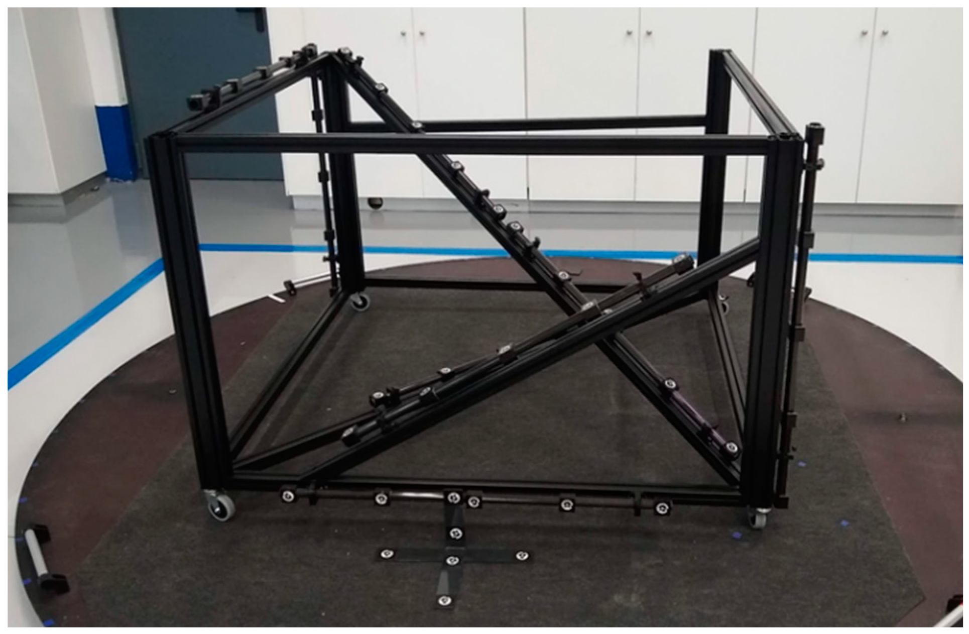
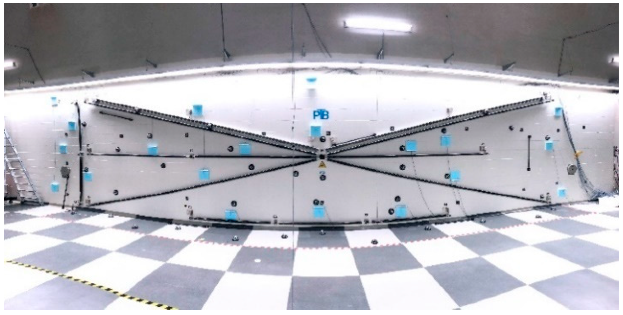
In addition to the photogrammetry system itself, a key component of this research is the test facility. In 2011, PTB established a reference wall to evaluate the length measurement capabilities of laser trackers, which are coordinate measuring systems (CMSs) widely used in large-volume metrology. The tests of the length measurement errors follow ISO 10360-10:2021 and VDI/VDE 2617 Part 10, which require either that measurements of calibrated measurement standards span a defined volume performed from a single position, or that a 2D arrangement of measurement standards be measured from at least seven specified positions to derive a volumetric length measurement error for the laser tracker. PTB has chosen to implement the latter of these two methods. The reference wall comprises a set of 15 magnetic nests mounted on a designated wall in PTB’s decommissioned nuclear reactor building; these nests create a large-scale 2D artefact (see Figure 2). The magnetic nests are attached to the wall via a setup of different spring blade elements to guarantee stress-free mounting and are connected via hollow carbon-fibre reinforced rods which have a low weight as well as a very low thermal expansion coefficient of only $\alpha =-1.0\cdot {10}^{-6}\dots -1.2\cdot {10}^{-6}{ \mathrm{K}}^{-1}$. Each of the magnetic nests is designed to hold a spherical target $38.1 \mathrm{mm} \left({1.5}^{″}\right)$ in diameter, which can be repeatedly positioned on three wedges on its perimeter. For different applications, a variety of targets are available such as polished and etched steel spheres, chalk-coated spheres, and sphere-mounted retroreflectors.

The reference wall allows the lengths between the nests to be calibrated with a comparably low calibration uncertainty. For this purpose, the individual lengths wee combined to form five groups: one vertical line (Line A), two diagonal lines (Lines B and C), and two horizontal lines (Lines D and E) at different heights of the wall. The lines connect either three or four nests (two or three calibrated lengths). Diagonal Lines B and C are approximately 12 m long, while Lines A, D, and E are about 3 m, 10 m, and 6 m long, respectively.

The individual lengths are calibrated by means of a self-tracking laser interferometer equipped with an environmental monitoring system which comprises sensors for the air temperature, the ambient air pressure, and the relative humidity. These sensors and the frequency of the laser’s light source are calibrated at PTB’s laboratories on a regular basis, thus ensuring a traceable calibration result. The measured lengths are corrected for the environmental influences on the air’s refractive index following the work of Edlén [29] and the refined equations of Bönsch and Potulski [30]. The calibration uncertainty of the lengths of the reference wall is $U\left(k=2\right)=20 \mathrm{\mu }\mathrm{m}$ or better.

3.2. Portable Photogrammetry Equipment

In this work, VSET, a commercial portable photogrammetry device manufactured by SORALUCE, has been used to represent portable photogrammetry. This device comprises a commercial Nikon D500 camera, a NIKON AF NIKKOR 24 MM F/2.8D prime lens, a NISSIN MF18 flashlight, six carbon fibre scale bars, several non-coded targets, coded targets, and a PC.

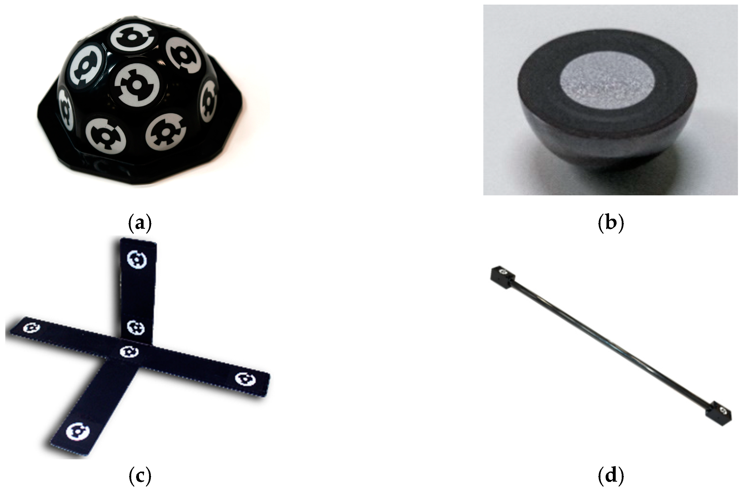
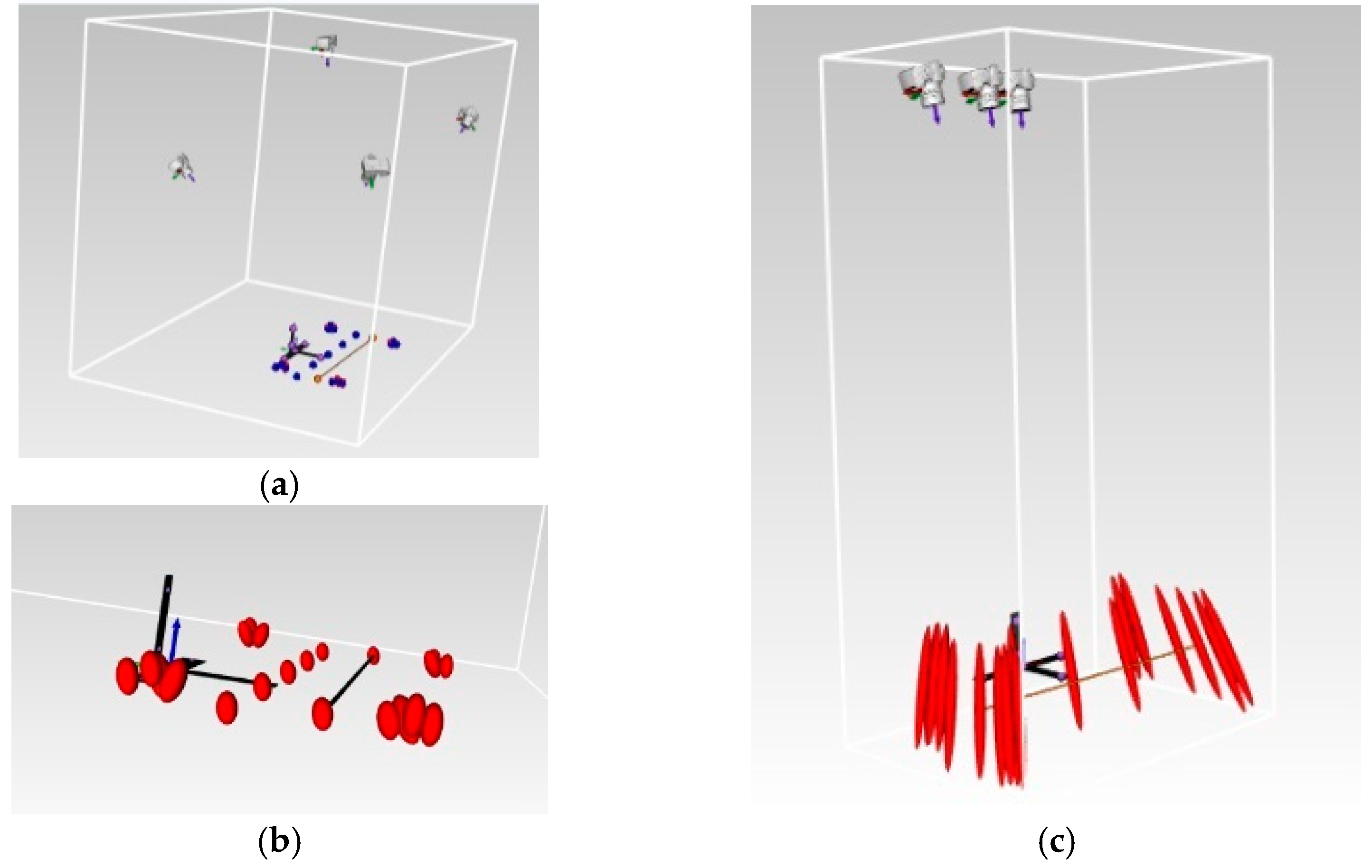
The coded targets are divided into three groups: one cross-point, the extremes of the scale bars, and 60 structures in the shape of an igloo, each of which is covered by 14 coded markers. The measurement starts from the cross-point (see Figure 3c) to reference the distances of the non-coded targets from the coordinate system’s origin. The origin is defined by six coded targets attached to the cross-point. The function of the scale bars is to provide the size reference of the measurement field (see Figure 3d). The distances between the coded markers have been calibrated using a Zeiss Accura CMM, thus ensuring the traceability of the measurement. Instead of a tactile probing system, an optical 2D image sensor (Zeiss ViScan) was used to measure the centre of the coded markers. To maintain the dimensions of the scale bars over time and to prevent thermal distortions, carbon fibre material was used to connect the markers at the extremes of the bar. The remaining coded targets were placed on the surfaces of 60 igloo-shaped structures to support the process of matching pictures (see Figure 3a) and computing the camera positions. The use of these elements is relevant because the image matching quality and the overall accuracy of the measurement process depends on an adequate distribution of the elements throughout the measurement field. As mentioned above, correct overlap between pictures is of utmost importance to allow the relative position of the cameras to be calculated with low uncertainty. The igloo-shaped structures allow the common point between the images to be identified in the first run and enable the software to assign a virtual label to the non-coded targets in order to identify them in the following pictures. Once the measurement has been finished, a second optimisation step is carried out to improve the position of the camera, the elements, and the non-coded and coded targets. Zatarain et al. and Mendikute et al. explained in detail all the algorithms needed to carry out a bundle adjustment in their research [27,28].

To use the photogrammetric system on the reference wall, a set of suitable targets is required which can be measured by means of photogrammetry while also fitting the nests at the calibrated lengths of the reference wall. For the measurements, 15 commercially available retroreflective targets centred on hemispherical balls (see Figure 3b) were used. The centring accuracy of the retroreflective target dots is specified as +/− 0.0127 mm by the manufacturer. The nominal diameter of the targets 38.1 mm (1.5″) is the same as the diameter of the sphere-mounted retroreflector used for the calibration of the reference wall. In this way, the calibrated distances between the nests can be directly compared with the results obtained from the photogrammetry measurements.

3.3. Method of Measuring the Reference Wall Using Photogrammetry

This study aimed to compare measurement techniques in a large-volume metrology scenario. As mentioned above, a reference wall is a suitable, independent, and readily available facility for carrying out this comparison. Previously, portable photogrammetry was accompanied by tests to design an optimal path planning procedure for the measurement of this facility (i.e., the reference wall). First, two tests validated the rules mentioned above concerning the placement of the elements and the positions from which the photos must be taken, respectively. In both cases, a simple scenario was designed to obtain the correct indications to apply when the path planning procedure for the reference wall was performed.

In accordance with these indications, three phases were defined. First, the elements were placed in such a way that robust extrinsic parameters were obtained from the target. Second, the user calculated the position of the auxiliary elements. Third, each target was captured from at least three positions in the shape of a triangle (triangulation).

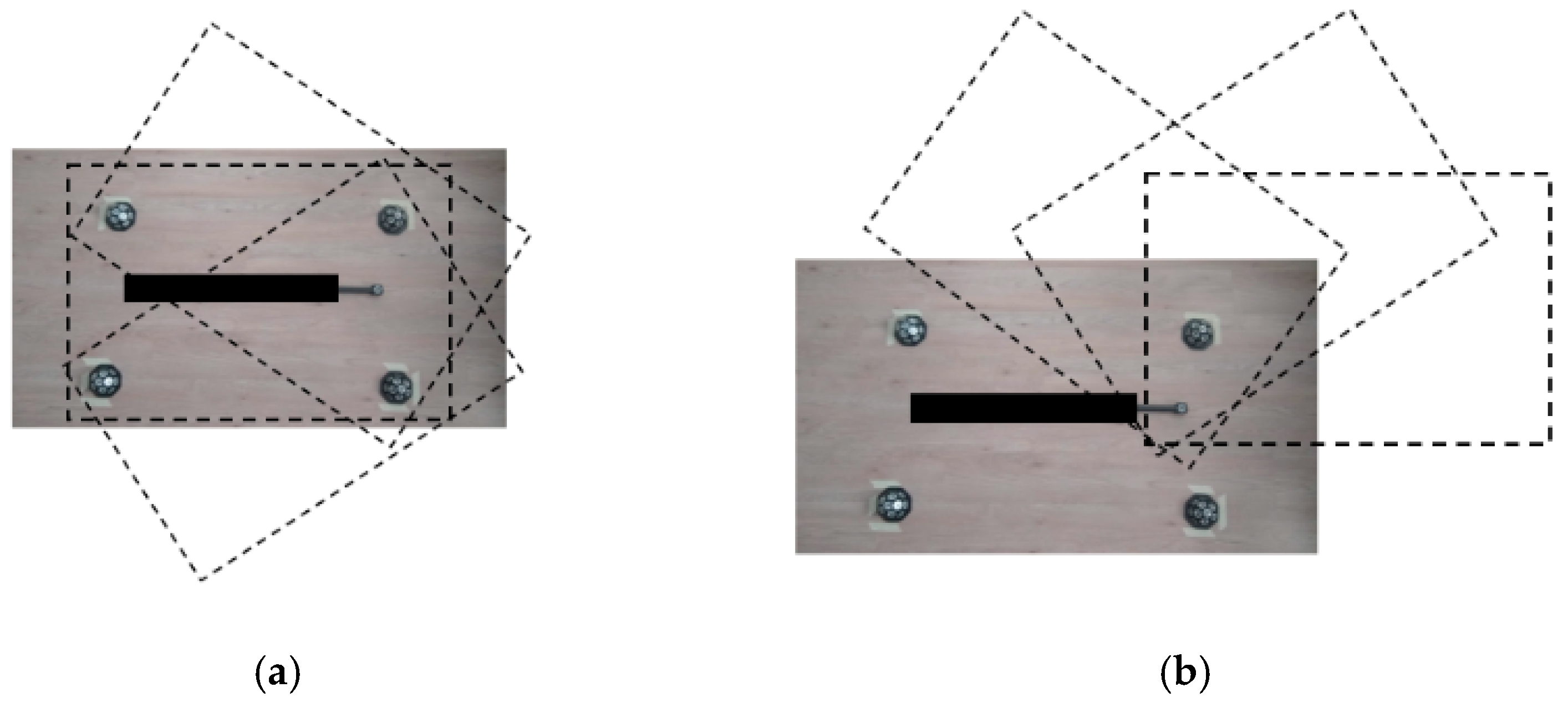
To show the importance of these variables, two levels of extrinsic parameters and two levels of the triangulation network were obtained using a down-scaled scenario to measure an artefact 1 m in length (see Figure 4). In the first case, one or three auxiliary elements were used to calculate the extrinsic parameters (position of the camera), while in the second case, the triangulation of the cameras (network) was changed from a narrow volume ($~0.1 {\mathrm{m}}^3$) to an optimal position based on the recommendation of 90° between the camera positions ($~3 {\mathrm{m}}^3$). Figure 5 shows both networks applied to measure a small-scale volume. Each case was repeated three times; the LME and its standard deviation are the results. To reduce the amount of information, only the average of each scenario is shown.

To complement the experimental results, a virtual model was simulated using the Monte Carlo method in order to analyse the uncertainty of two processes: the 6-degree-of-freedom (6DoF) camera pose calculation, and the optical target 3D coordinate computation by triangulation. Each one of the processes was simulated independently, so that the first qualitative evaluation was performed on the influence of the relevant process variables (i.e., the spatial 3D arrangement of the auxiliary optical targets for 6DoF camera pose computation, and the relative 6DoF camera poses for 3D optical target computation by triangulation). The inherent covariance in portable photogrammetry between the 6DoF camera poses and 3D target coordinates was not considered in these simulations. Target detection uncertainty was adopted as the main error source to propagate in the Monte Carlo simulation of each process. Image detection uncertainty was estimated at 0.1 pixel (standard deviation), according to the mean retroprojection error observed in the residual error distribution of the joined bundle of the self-calibrated portable photogrammetry minimisation problem. An even detection uncertainty was assumed, regardless of the target size and location at the image plane, for all targets in all images.

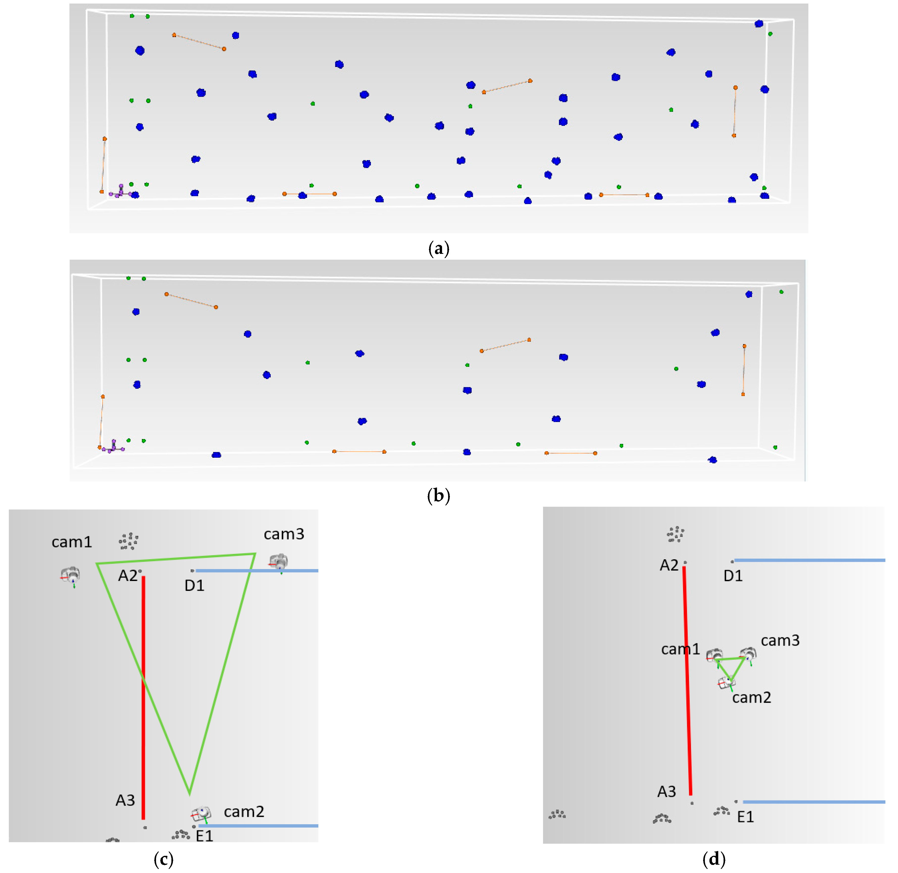
This simulation tool converts the estimate validated in a small-scale scenario into large scales to reduce the number of trials required. Figure 5 shows red ellipses with the shape of the uncertainty considering the influence of the camera positions, which are the key variables for an optimal network configuration. If the relative positions between the points of view create a pyramid shape (an efficient network) where one vertex is the target, the estimated uncertainty is reduced [9]. If the relative positions are quite close among the points of view (a deficient network), the estimated uncertainty is oriented to the centre of the positions and is larger than for the previous situation.

The plan carried out to measure the reference wall was divided into four different conditions or scenarios (see Figure 5). Each condition was measured three times to obtain a reliable result. The expected results are shown in

Table 1. Results expected for the measurements of the reference wall from the four scenarios investigated.

	Efficient Network	Deficient Network
Extrinsic parameter: high number of references	Best Scenario 1	Intermediate Scenario 2
Extrinsic parameter: low number of references	Intermediate Scenario 3	Worst Scenario 4

.

Figure 6a shows the positions where auxiliary elements must be placed to obtain a robust extrinsic parameter. Using these elements, two networks were tested: Figure 6c (an efficient network) and Figure 6d (a deficient network in which the camera positions were closer to each other). Some of the auxiliary elements were then removed from the wall, leaving Figure 6b. Afterwards, the efficient and deficient network measurements were repeated with fewer auxiliary elements. The number of auxiliary elements was chosen to represent a measurement in the case of the minimum number of elements (low-level scenario), while creating a dense network of auxiliary elements for the high-level scenarios (14 and 33 auxiliary elements, respectively). Although it would have been possible to quantify this second variable, concrete values were selected on the basis of experience.

4. Results

As explained in the previous section, before taking the measurements of the reference wall, two downscaled tests were carried out using a smaller measurement volume to prepare for the measurements; this had the added benefit of reducing the number of trials required.

The first test was performed to demonstrate the influence of the number of auxiliary elements used on the uncertainty of the measurement process. The difference in the observed standard deviations of the LME, as shown in

Table 2. Comparison between the experimental results and simulations comparing the influence of auxiliary elements with respect to the standard deviation of the maximum LME and the average of the maximum error.

	Experimental	Simulated
LME σ (+/− mm) k = 2
Low number of auxiliary elements	0.662	2.764
High number of auxiliary elements	0.102	0.162
$\overline{x}$ (mm)
Low number of auxiliary elements	−0.110	−0.545
High number of auxiliary elements	−0.039	−0.068

, underlines the importance of calculating the targets’ positions using sufficient auxiliary elements. Furthermore, the simulations used to validate the design of the path planning procedure predicted the correct trend, although they were not able to reproduce the exact values. For the Monte Carlo simulations, the image detection uncertainty was considered to be the main uncertainty contribution, assuming a normal distribution with the standard deviation of $\sigma =0.1 \mathrm{pixel}$.

When we considered the differences between the two network scenarios investigated (efficient and deficient), the results were quite similar to those of the previous test. The results in Table 2 show a reduction in the deviation when using an efficient network; however, the improvement is minimal, given the influence of the number of auxiliary elements used.

After evaluating the predictions of the simulations, measurements of the reference wall were carried out accordingly. Figure 7 and

Table 3. Comparison between the experimental results and simulations, comparing the influence of the network with respect to the standard deviation of the maximum LME and the average maximum error.

	Experimental	Simulated
LME σ (+/− mm) k = 2
Deficient network	0.236	0.300
Efficient network	0.074	0.118
$\overline{x}$ (mm)
Deficient network	0.264	0.194
Efficient network	0.072	0.064

show a summary of the results. The average number of photos per test was 230 in Scenario 1, 185 in Scenario 2, 130 in Scenario 3, and 125 in Scenario 4.

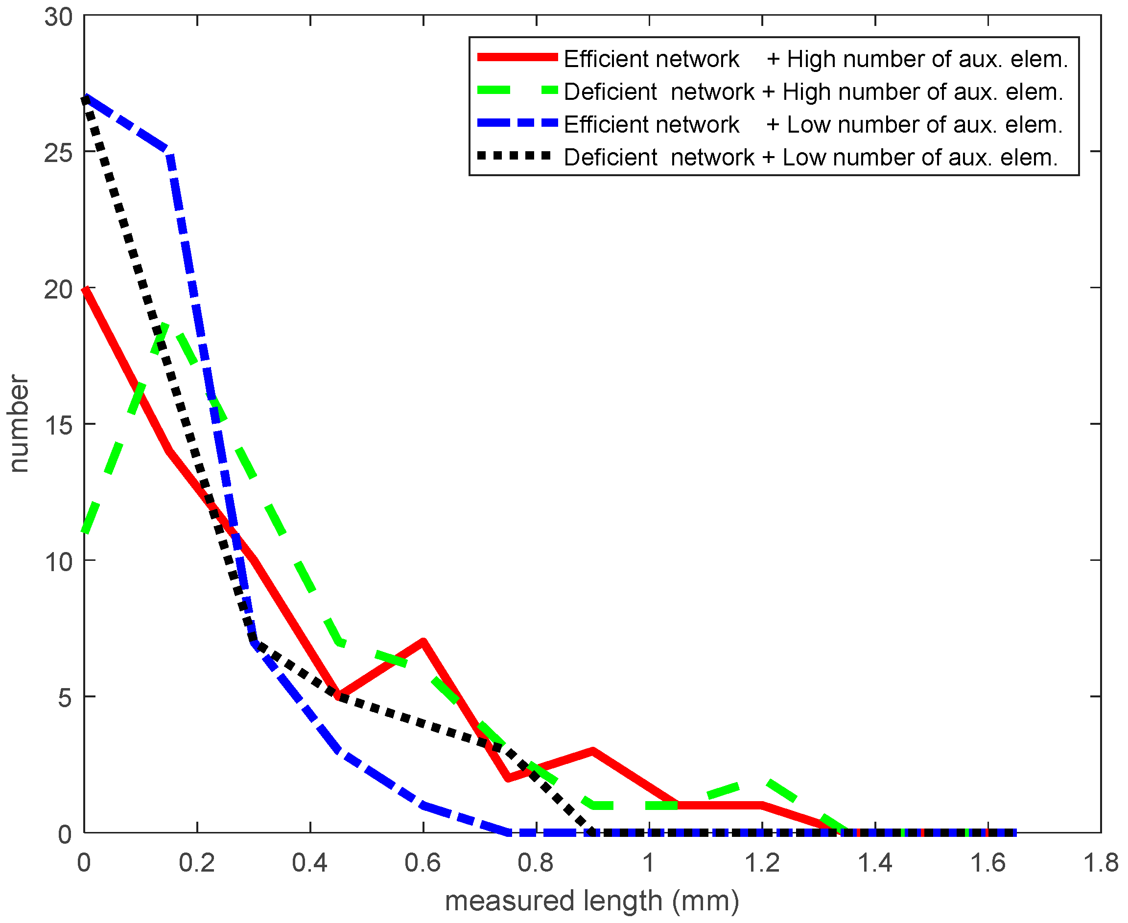
If we examine the results obtained (Table 3), there is a trend that was not anticipated by the expected results (Table 1). The efficient network shows poorer results than the deficient network. This trend will be discussed in the next section, as well as the outliers at the centre of Figure 8 (at a measured length of approx. $6 \mathrm{m}$).

The average time used for measuring the reference wall was approximately 1 h with an additional hour to place the elements and set up the camera.

As mentioned in the previous section, one of the studied variables did not follow the expected trend. The LME and the average error between the high and low numbers of auxiliary elements contradicts the expected behaviour predicted in Figure 8. Studying the procedures of the tests allowed a possible reason for the results to be identified. In Scenarios 1 and 2, the user took photos at a closer distance than in Scenarios 3 and 4, as this was possible due to the number of auxiliary elements (see

Table 4. Results of the trials for the efficient and deficient networks using low-level and high-level extrinsic parameters.

(mm)	High-Level Extrinsic Parameters				Low-Level Extrinsic Parameters
	Efficient network		Deficient network		Efficient network		Deficient network
	Scenario 1		Scenario 2		Scenario 3		Scenario 4
Test	$\overline{x}$	LME	$\overline{x}$	LME	$\overline{x}$	LME	$\overline{x}$	LME
1	0.165	0.775	0.440	1.281	0.262	0.729	0.261	0.834
2	0.315	0.959	0.274	0.589	0.187	0.517	0.271	0.773
3	0.572	1.229	0.450	1.206	0.139	0.382	0.208	0.858

to identify the scenarios). Consequently, an excessive drift may have been generated, which would have resulted in larger length measurement errors.

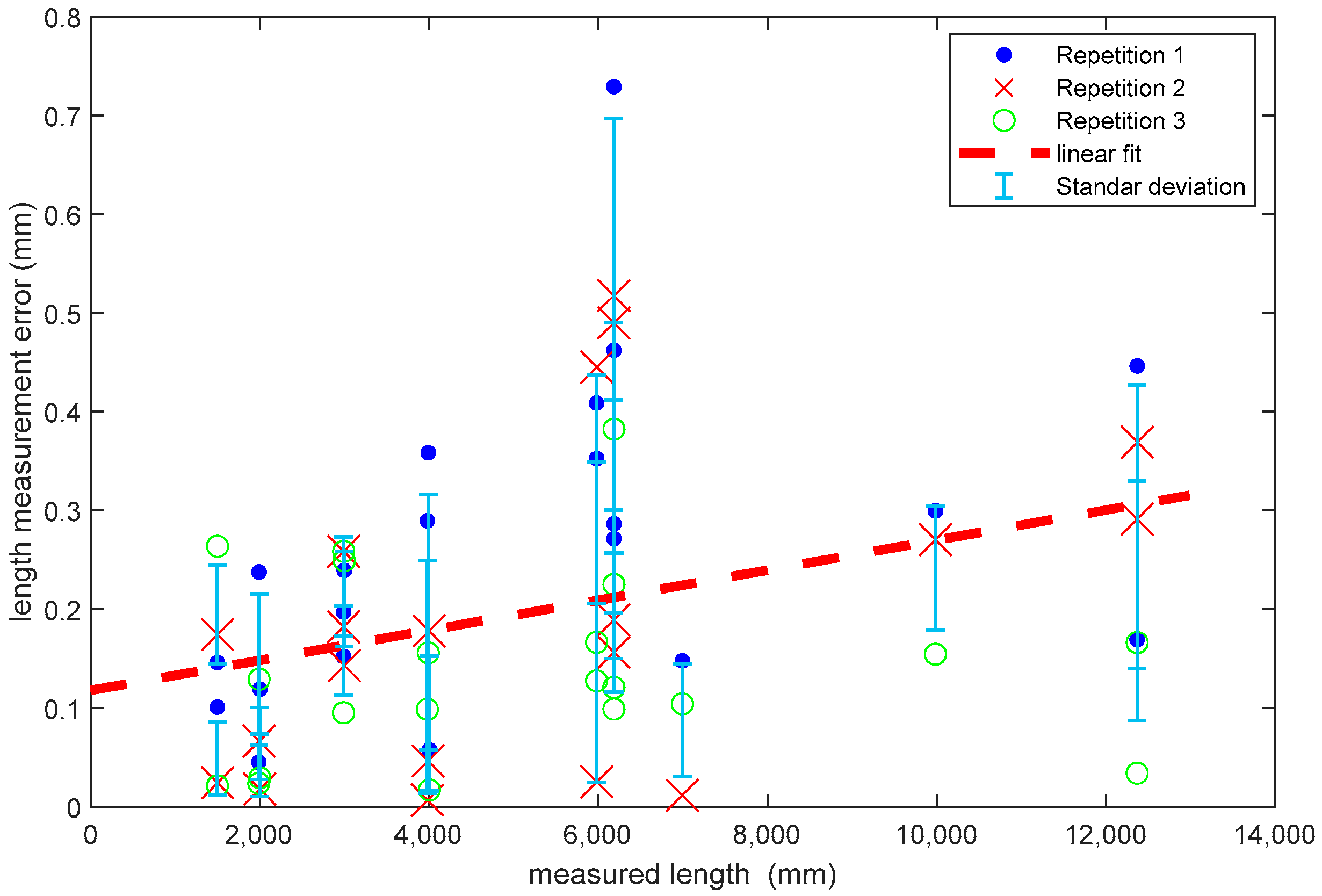
An additional deviation requires explanation: As can be seen in Figure 8, the linear trend of the length dependency of the observed errors shows significant scatter and a deviation at approximately $6 \mathrm{m}$ in length. All the points which take the centre point of the measurement standards of the reference wall into account deviate from the linear trend (as well as some other points). Here, the positions of the auxiliary elements and the number of photos of this target are the likely cause of this deviation. The user took more photos of the outlying regions of the reference wall than of the centre, as there were more elements in these regions.

However, the rest of the deviation shows an increasing trend with an increase in the measured length. Furthermore, an improvement resulting from the choice of the network can be observed.

Moreover, a novice (less experienced) user carried out the experiments, so the results were not significantly affected by the user’s knowledge. Nevertheless, after finding a different trend than expected, two corrections were suggested by an experienced photogrammetry user; after implementing these corrections, Scenario 1 was repeated. The first suggestion was to take photographs at greater distances, since the user took photos in Scenario 1 and 2 at closer distances than in Scenario 3 and 4. The system provider issued a guideline to less experienced users to modify the number of auxiliary elements while maintaining the approximate distance during the measurement of the reference wall. The second suggestion was to increase the number of photos taken from the highest position because, in the first set of measurements, the operator used a ladder, but only at the corners of the reference wall.

The results show an improvement in terms of the average error and LME with respect to Scenario 1 (see

Table 5. Results of the repetition of Scenario 1 with high-level extrinsic parameters and an efficient network.

Repetition		1	2
Efficient network	$\overline{x} \left(\mathrm{mm}\right)$	0.181	0.169
S1 Repetition	LME (mm)	0.435	0.350

). Considering the repetition for Scenario 1, the results show the expected trend of less deviation with respect to the nominal length using the combination of high-level extrinsic parameters and an efficient network.

5. Discussion

If we consider the results of these 14 trials under the conditions studied, the network can be identified as the variable with the greatest influence on the accuracy of the measurement process (i.e., with a greater influence than the number of auxiliary elements). However, considering both variables will always improve the photogrammetry results. For example, to measure the wing of an aeroplane or the blades of a wind turbine, it is advisable to ensure a uniform distribution of auxiliary elements with approximately one auxiliary element (see Figure 3) per ${\mathrm{m}}^2$ and four pictures. Furthermore, the user must ensure that the photos are taken from an appropriate distance (roughly $3 \mathrm{m}$ is advisable). However, the remaining recommendations must also be followed, such as sufficient overlapping and the choice of a strong network. Complex geometries may require the different points of view to be studied in greater detail to obtain a reliable solution.

Table 6. Performance summary of the datasets to evaluate the capabilities of the photogrammetry system used.

	Portable Photogrammetry
LME up to 12 m	Best of 3 repetitions 0.350 mm Average of 3 repetitions 0.542 mm
Average error (mm)	$0.117+\mathrm{L}$0.015
Preparation time	1 h
Measuring time	1 h
Auxiliary elements	15
Scale bars	6
Number of images per test	130

contains a proposal for reporting the capabilities of portable photogrammetry systems. Here, the following points should be included: the length measurement error, the average error, the preparation time, and the measuring time. This enables the user to evaluate the system by comparing these four parameters. Furthermore, it can be useful to provide the number of auxiliary elements, the number of scale bars, and the number of images. Although the training time also constitutes key information, this parameter significantly depends on the operator. For the portable photogrammetry system used in this study, users currently need between one and two hours to start measuring, and two days of lessons to learn to avoid the most common mistakes and possible ways to avoid them. In the case that users do not know how to interpret metrological data, extra training will be needed.

This table provides additional and complementary information to that reported by Martin et al. [14] when comparing different portable photogrammetry systems with a laser-tracker. Indeed, despite the uncertainty figures estimated for each work are not directly comparable (LME values in this work and the spatial coordinate errors used by Martin et al.), it should be noted that the evaluation results obtained here are consistent and in the same order of magnitude to those observed previously by [14].

6. Conclusions

Portable photogrammetry is a measurement technology with high potential for measuring large-scale volumes with high accuracy, but validating the performance of the system for these dimensions is difficult. In this study, the potential of portable photogrammetry was demonstrated by measuring an artefact comprising measurement standards up to 12 m in length. To guide users in the evaluation of the photogrammetry systems, a table to report the results has been proposed that will simplify the comparison of different portable photogrammetry systems under similar conditions. The artefact used allows distances in the same LVM range to be measured; thus, portable photogrammetry should be tested in a more suitable way than with smaller artefacts only.

Moreover, to test the influence of the user, measurements were carried out in different scenarios. The simplicity of portable photogrammetry for measuring large-scale volumes is a double-edged sword because, while it is easy to obtain results, their accuracy may be unsatisfactory—a situation which is far from optimal if undetected. Good practices have been explained to help users achieve the best possible results.

Focussing on the interface between the user and the system, this research has investigated how to correctly use the auxiliary elements and calculate robust camera positions, and how the correct network of camera positions (triangulation) reduces the uncertainty of the calculated target positions. These aspects help to ensure that the successful use of photogrammetry is dependent on the user’s skills only to a small extent.

Portable photogrammetry has high potential to be used for LVM measurements, as do laser-based methods, but only when good practices are followed.

References

1. Savio, E.; De Chiffre, L.; Schmitt, R. Metrology of freeform shaped parts. CIRP Ann. Manuf. Technol. 2007, 56, 810–835. [Google Scholar] [CrossRef]
2. Hughes, B.; Forbes, A.; Sun, W.; Veal, D.; Nasr, K. Determination of misalignment and angular scale errors of a laser tracker using a new geometric model and a multi-target network approach. In Proceedings of the MacroScale 2011, Wabern, Switzerland, 4–6 October 2011; Available online:https://www.semanticscholar.org/paper/Determination-of-misalignment-and-angular-scale-of-Lewis-Hughes/bfc07c667c64ec4865ff12713379f393bfdbd5ff (accessed on 31 March 2022).
3. Heaps, J.; Hughes, B. Refinements and introduction of photogrammetric elements to an experimental trilateration based optical metrology system. Int. Arch. Photogramm. Remote Sens. Spat. Inf. Sci. ISPRS Arch. 2020, 43, 771–776. [Google Scholar] [CrossRef]
4. Rafeld, E.K.; Koppert, N.; Franke, M.; Keller, F.; Heisselmann, D.; Stein, M.; Kniel, K.; Heißelmann, D.; Stein, M.; Kniel, K. Recent developments on an interferometric multilateration measurement system for large volume coordinate metrology. Meas. Sci. Technol. 2021, 33, 035004. [Google Scholar] [CrossRef]
5. Guillory, J.; Truong, D.; Wallerand, J.-P. Multilateration with Self-Calibration: Uncertainty Assessment, Experimental Measurements and Monte-Carlo Simulations. Metrology 2022, 2, 241–262. [Google Scholar] [CrossRef]
6. Pfeifer, T.; Montavon, B.; Peterek, M.; Hughes, B. Artifact-free coordinate registration of heterogeneous Large-Scale Metrology systems. CIRP Ann. 2019, 68, 503–506. [Google Scholar] [CrossRef]
7. Nitsche, J.; Franke, M.; Haverkamp, N.; Heißelmann, D. Six-degree-of-freedom pose estimation with μm/μrad accuracy based on laser multilateration. J. Sens. Sens. Syst. 2021, 10, 19–24. [Google Scholar] [CrossRef]
8. Galetto, M.; Mastrogiacomo, L.; Pralio, B. MScMS-II: An innovative IR-based indoor coordinate measuring system for large-scale metrology applications. Int. J. Adv. Manuf. Technol. 2011, 52, 291–302. [Google Scholar] [CrossRef] [Green Version]
9. Luhmann, T.; Robson, S.; Kyle, S.; Boehm, J. Close-Range Photogrammetry and 3D Imaging. Close Range Photogramm. 3d Imaging 2019, 7, 445–480. [Google Scholar] [CrossRef]
10. Kröger, L.; Wester, T.T.B.; Langidis, A.; Nietiedt, S.; Göring, M.; Luhmann, T.; Peinke, J.; Hölling, M.; Gülker, G. Experimental study of fluid-structure interaction at a model wind turbine blade using optical measurement techniques. J. Phys. Conf. Ser. 2020, 1618. [Google Scholar] [CrossRef]
11. Filion, A.; Joubair, A.; Tahan, A.S.; Bonev, I.A. Robot calibration using a portable photogrammetry system. Robot. Comput. Integr. Manuf. 2018, 49, 77–87. [Google Scholar] [CrossRef]
12. Boby, R.A. Kinematic Identification of Industrial Robot Using End-Effector Mounted Monocular Camera Bypassing Measurement of 3-D Pose. IEEE/ASME Trans. Mechatron. 2022, 27, 383–394. [Google Scholar] [CrossRef]
13. Mendikute, A.; Leizea, I.; Herrera, I. In-process portable photogrammetry using optical targets for large scale industrial metrology. In Proceedings of the 19th International Conference & Exhibition, Bilbao, Spain, 3–7 June 2019. [Google Scholar]
14. Martin, O.C.; Robson, S.; Kayani, A.; Muelaner, J.E.; Dhokia, V.; Maropoulos, P.G. Comparative Performance between Two Photogrammetric Systems and a Reference Laser Tracker Network for Large-Volume Industrial Measurement. Photogramm. Rec. 2016, 31, 348–360. [Google Scholar] [CrossRef] [Green Version]
15. Geodetic Geodetic Reports. Available online: https://www.geodetic.com/resources/reports/ (accessed on 29 April 2022).
16. Luhmann, T. Close range photogrammetry for industrial applications. ISPRS J. Photogramm. Remote Sens. 2010, 65, 558–569. [Google Scholar] [CrossRef]
17. Carmignato, S.; De Chiffre, L.; Bosse, H.; Leach, R.; Balsamo, A.; Estler, W. Dimensional artefacts to achieve metrological traceability in advanced manufacturing. CIRP Ann. Manuf. Technol. 2020, 69, 693–716. [Google Scholar] [CrossRef]
18. Hastedt, H. Monte-Carlo-Simulation In Close-Range Photogrammetry. Int. Arch. Photogramm. Remote Sens. Spat. Inf. Sci. 2004. Available online: https://www.isprs.org/proceedings/XXXV/congress/comm5/papers/515.pdf (accessed on 31 March 2022).
19. Luhmann, T. Precision potential of photogrammetric 6DOF pose estimation with a single camera. ISPRS J. Photogramm. Remote Sens. 2009, 64, 275–284. [Google Scholar] [CrossRef]
20. Hastedt, H.; Luhmann, T.; Przybilla, H.J.; Rofallski, R. Evaluation of interior orientation modelling for cameras with aspheric lenses and image pre-processing with special emphasis to SFM reconstruction. Int. Arch. Photogramm. Remote Sens. Spat. Inf. Sci. ISPRS Arch. 2021, 43, 17–24. [Google Scholar] [CrossRef]
21. Zhou, S.; Zhu, H.; Ma, Q.; Ma, S. Mechanism and compensation of measurement error induced by thermal deformation of digital camera in photo mechanics. Appl. Sci. Switz. 2020, 10, 3422. [Google Scholar] [CrossRef]
22. Mendikute, A.; Yagüe-Fabra, J.A.; Zatarain, M.; Bertelsen, Á.; Leizea, I. Self-Calibrated In-Process photogrammetry for large raw part measurement and alignment before machining. Sens. Switz. 2017, 17, 2066. [Google Scholar] [CrossRef] [Green Version]
23. Dunn, E.; Frahm, J.M. Next best view planning for active model improvement. In Proceedings of the British Machine Vision Conference, BMVC 2009, Cambridge, UK, 7–10 September 2009. [Google Scholar]
24. Cullen, S.; Mackay, R.; Mohagheghi, A.; Du, X. The Use of Smartphone Photogrammetry to Digitise Transtibial Sockets: Optimisation of Method and Quantitative Evaluation of Suitability. Sensors 2021, 21, 8405. [Google Scholar] [CrossRef]
25. Ali Hosseininaveh, A.; Sargeant, B.; Erfani, T.; Robson, S.; Shortis, M.; Hess, M.; Boehm, J. Towards fully automatic reliable 3D acquisition: From designing imaging network to a complete and accurate point cloud. Robot. Auton. Syst. 2014, 62, 1197–1207. [Google Scholar] [CrossRef]
26. Sandwith, S.; Cork, G. V-Stars/M System Accuracy Test Results. In Proceedings of the Coordinate Measurement System Committee, Michigan, MI, USA, 31 July–4 August 2000. [Google Scholar]
27. Zatarain, M.; Mendikute, A.; Inziarte, I. Raw part characterisation and automated alignment by means of a photogrammetric approach. CIRP Ann. Manuf. Technol. 2012, 61, 383–386. [Google Scholar] [CrossRef]
28. Mendikute, A.; Leizea, I.; Yagüe-Fabra, J.A.; Zatarain, M. Self-calibration technique for on-machine spindle-mounted vision systems. Meas. J. Int. Meas. Confed. 2018, 113, 71–81. [Google Scholar] [CrossRef] [Green Version]
29. Edlén, B. The refractive index of air. Metrologia 1966, 2, 71–80. [Google Scholar] [CrossRef]
30. Bönsch, G.; Potulski, E. Measurement of the refractive index of air and comparison with modified Edlén’s formulae. Metrologia 1998, 35, 133–139. [Google Scholar] [CrossRef]
Figure 1. An arrangement of the reference scale bars for testing optical 3D measuring systems in accordance with VDI/VDE 2634 Part 1.
Metrology 02 00020 g001
Figure 2. A photograph of PTB’s reference wall with the installed targets and markers for the photogrammetry system being tested. The maximum length is approximately 12 m (diagonals).
Metrology 02 00020 g002
Figure 3. (a) The igloo-shaped auxiliary element with coded markers. At the bottom, there are three magnets for attaching the element to ferromagnetic workpieces. (b) A retroreflective target on a hemisphere for use with the nests on the reference wall (target diameter: 20   mm ). (c) Cross-point providing the coordinate system’s origin. (d) Scale bars with coded markers ensure the correct scale of the measurement field.
Metrology 02 00020 g003
Figure 4. Relevance of the auxiliary elements: (a) A robust camera position can only be obtained if three or more auxiliary elements have been covered by the photographs (dashed lines). (b) Example of a weak camera position resolution using one auxiliary element.
Metrology 02 00020 g004
Figure 5. Network relevance: (a) An efficient network generates a narrow uncertainty (red ellipses). (b) Detailed view of (a). (c) A deficient network produces considerably larger uncertainty.
Metrology 02 00020 g005
Figure 6. Simulation of the reference wall measurement scenarios: (a) layout of the auxiliary elements (large blue dots), scale bars (red lines), and targets of the reference wall (small green dots) for measurements with a high number of auxiliary elements; (b) layout for measurements with a low number of auxiliary elements (note the number of auxiliary elements has been reduced from 33 to 14); (c) detailed schematic from the front view for measuring the reference wall’s length (A2 to A3) using an efficient network.(d) Detailed schematic from the front view for measuring a reference wall’s length (A2 to A3) using a deficient network.
Metrology 02 00020 g006
Figure 7. Distribution of the observed length measurement errors without showing their dependency on the measured distance.
Metrology 02 00020 g007
Figure 8. Errors of the deficient network and high-level extrinsic parameters.
Metrology 02 00020 g008