
Outlier Elimination in Rough Surface Profilometry with Focus Variation Microscopy


Abstract
:1. Introduction
1.1. Background of Focus Variation Technology
1.2. Motivation Statement
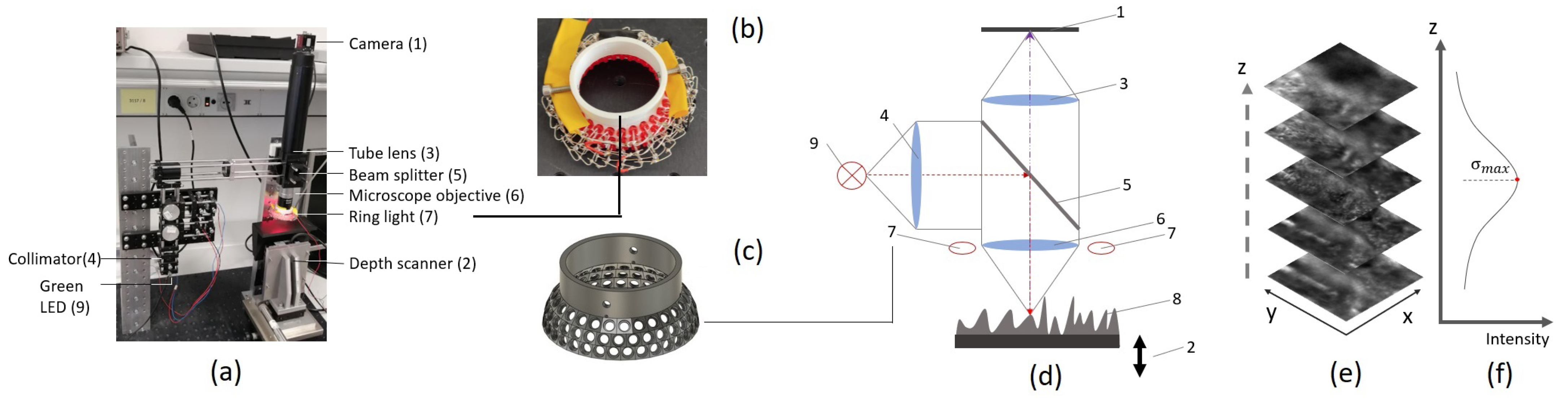
2. System Setup
3. Methodology
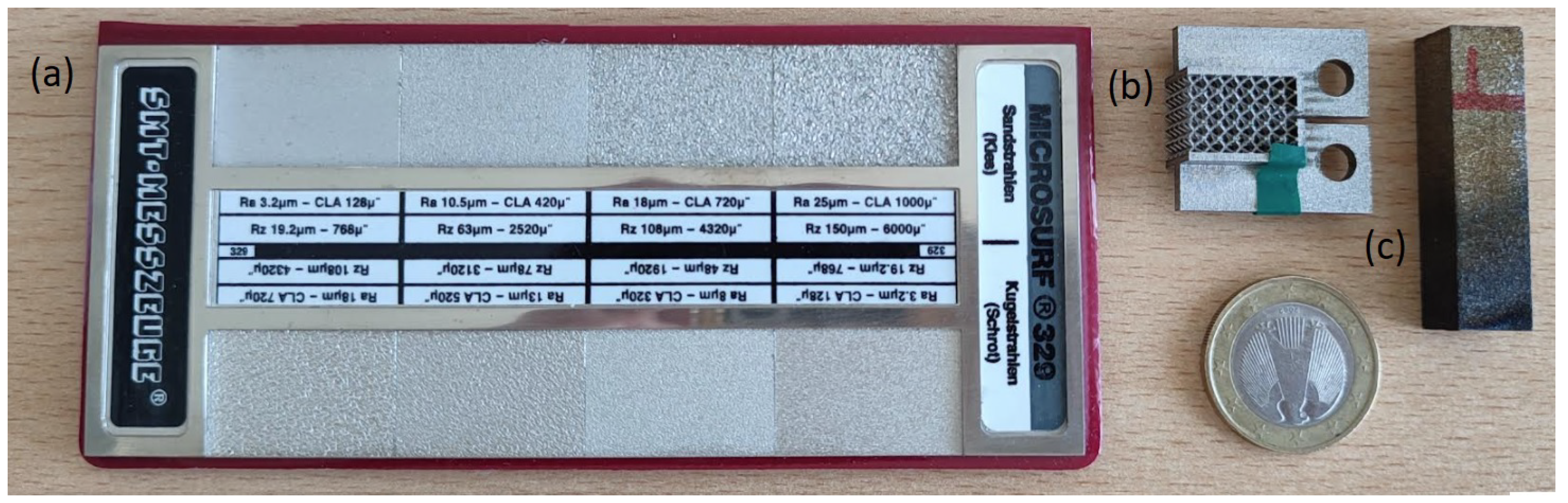
3.1. Samples
3.2. Data Preparation
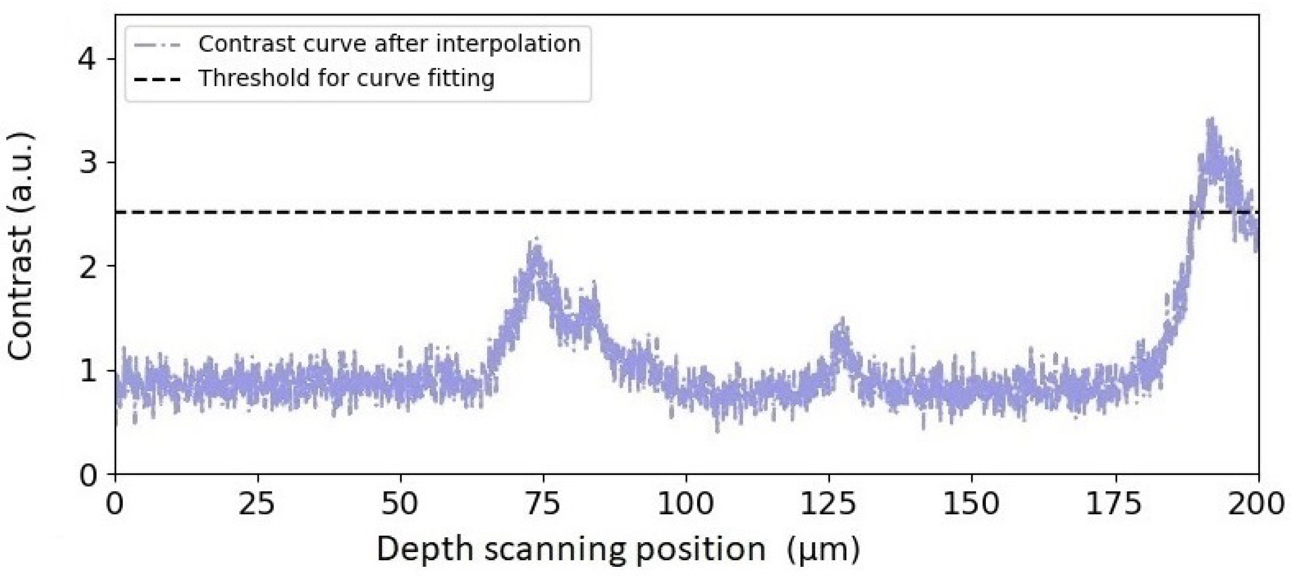
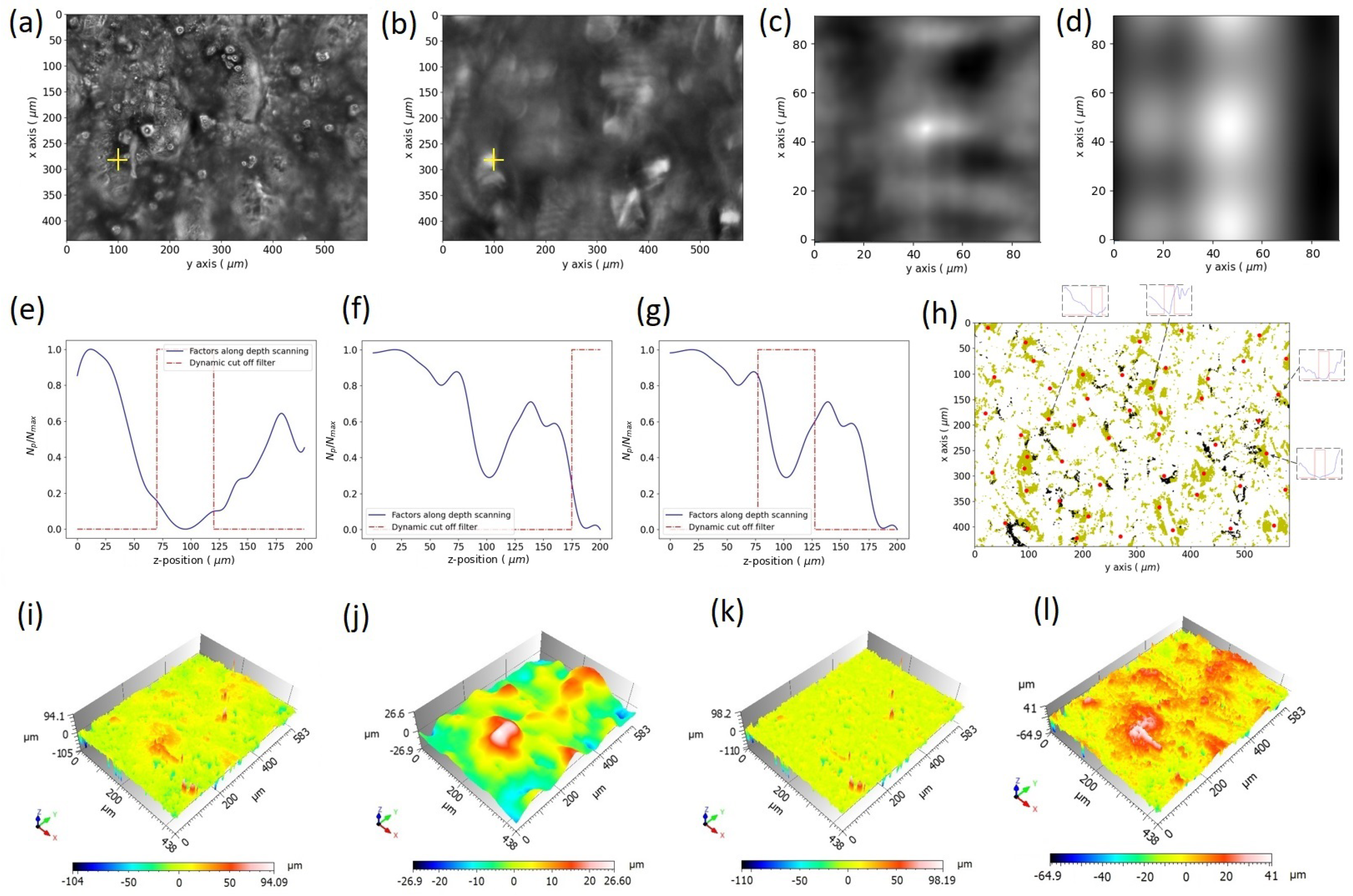
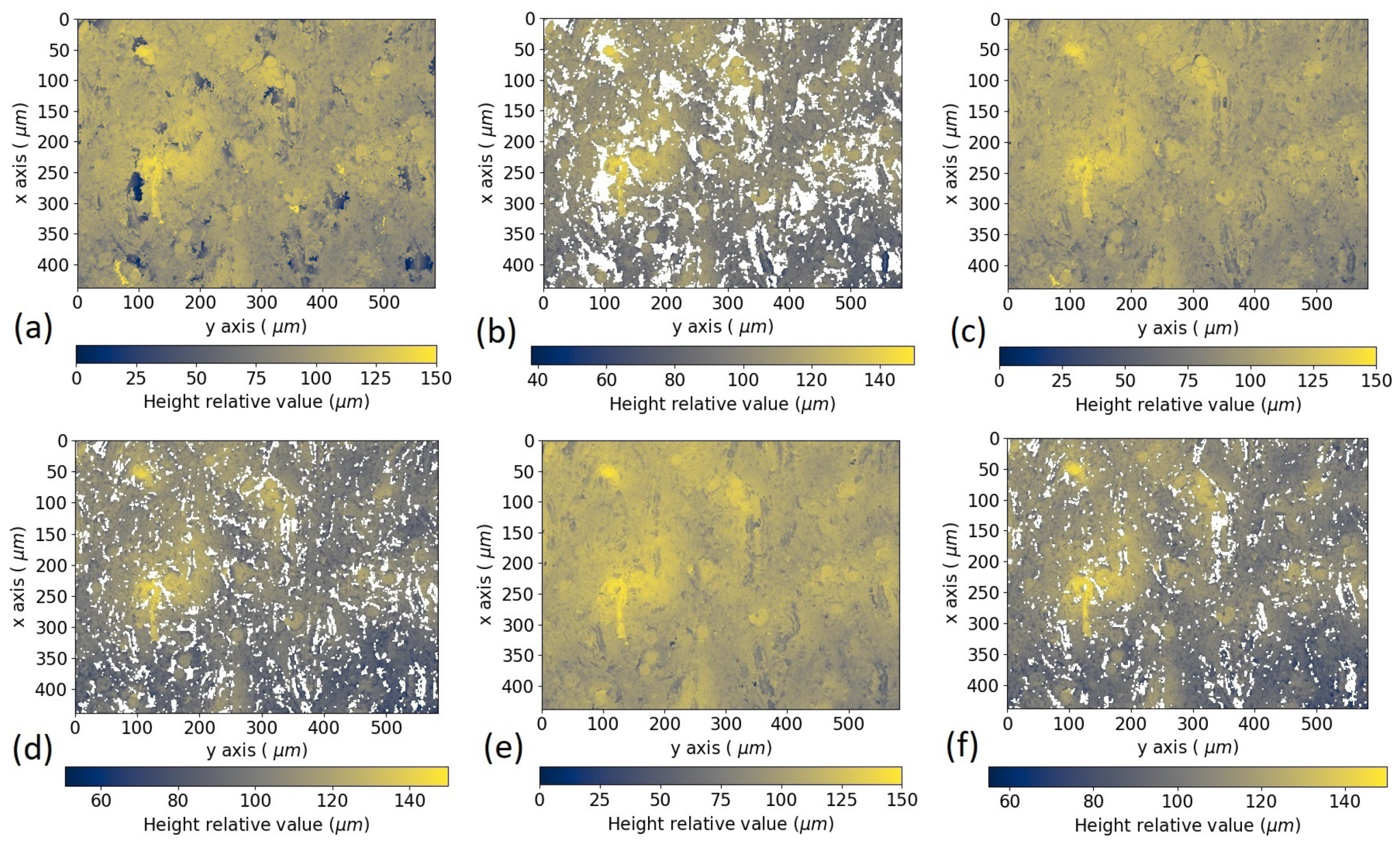
3.3. Artifact Analysis and Data Postprocessing
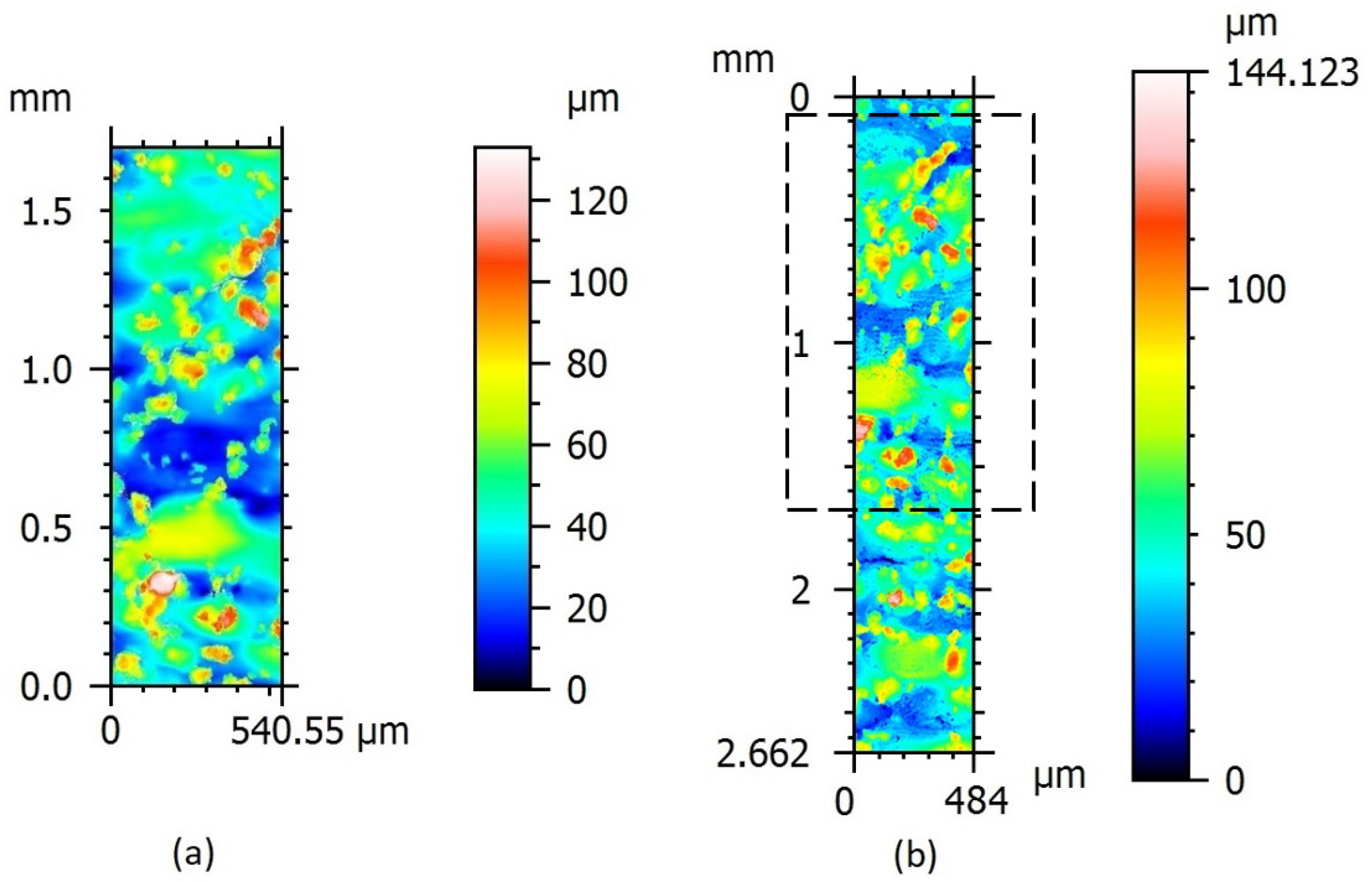
4. Measurement Results
4.1. Comparison of Topographies before and after Using ACF Filter and Different Exposure Times
4.2. Validation with Rubert Microsurf 329 Comparator Test Panel
4.3. Measurement of MA Surface
5. Conclusions
Author Contributions
Funding
Institutional Review Board Statement
Informed Consent Statement
Data Availability Statement
Conflicts of Interest
References
- Tapia, G.; Elwany, A. A review on process monitoring and control in metal-based additive manufacturing. J. Manuf. Sci. Eng. 2014, 136, 060801. [Google Scholar] [CrossRef]
- Mueller, B. Additive manufacturing technologies—Rapid prototyping to direct digital manufacturing. Assem. Autom. 2012, 32, 1–18. [Google Scholar] [CrossRef]
- Newton, L.; Senin, N.; Gomez, C.; Danzl, R.; Helmli, F.; Blunt, L.; Leach, R. Areal topography measurement of metal additive surfaces using focus variation microscopy. Addit. Manuf. 2019, 25, 365–389. [Google Scholar] [CrossRef]
- Townsend, A.; Senin, N.; Blunt, L.; Leach, R.; Taylor, J. Surface texture metrology for metal additive manufacturing: A review. Precis. Eng. 2016, 46, 34–47. [Google Scholar] [CrossRef] [Green Version]
- Gibson, I.; Rosen, D.; Stucker, B.; Khorasani, M. Additive Manufacturing Technologies; Springer: Berlin/Heidelberg, Germany, 2014. [Google Scholar]
- Whitehouse, D. Stylus contact method for surface metrology in the ascendancy. Meas. Control 1998, 31, 48–50. [Google Scholar] [CrossRef]
- Hillmann, W.; Kranz, O.; Eckolt, K. Reliability of roughness measurements using contact stylus instruments with particular reference to results of recent research at the Physikalisch-Technische Bundesanstalt. Wear 1984, 97, 27–43. [Google Scholar] [CrossRef]
- Safdar, A.; He, H.; Wei, L.; Snis, A.; Paz, L. Effect of process parameters settings and thickness on surface roughness of EBM produced Ti-6Al-4V. Rapid Prototyp. J. 2012, 3, 401–409. [Google Scholar] [CrossRef]
- Grimm, T.; Wiora, G.; Witt, G. Characterization of typical surface effects in additive manufacturing with confocal microscopy. Surf. Topogr. Metrol. Prop. 2015, 3, 014001. [Google Scholar] [CrossRef]
- Townsend, A.; Pagani, L.; Scott, P.; Blunt, L. Areal surface texture data extraction from X-ray computed tomography reconstructions of metal additively manufactured parts. Precis. Eng. 2017, 48, 254–264. [Google Scholar] [CrossRef]
- Townsend, A.; Blunt, L.; Bills, P. Investigating the capability of microfocus x-ray computed tomography for areal surface analysis of additively manufactured parts. In Proceedings of the American Society for Precision Engineering Summer Topical Meeting: Dimensional Accuracy and Surface Finish in Additive Manufacturing, Raleigh, NC, USA, 27–30 June 2016. [Google Scholar]
- Kerckhofs, G.; Pyka, G.; Moesen, M.; Van Bael, S.; Schrooten, J.; Wevers, M. High-resolution microfocus X-ray computed tomography for 3D surface roughness measurements of additive manufactured porous materials. Adv. Eng. Mater. 2013, 15, 153–158. [Google Scholar] [CrossRef]
- Danzl, R.; Helmli, F.; Scherer, S. Focus variation—A robust technology for high resolution optical 3D surface metrology. Stroj.-Vestn.-J. Mech. Eng. 2011, 57, 245–256. [Google Scholar] [CrossRef] [Green Version]
- Tian, Y.; Weckenmann, A.; Hausotte, T.; Schuler, A.; He, B. Measurement strategies in optical 3-D surface measurement with focus variation. In Proceedings of the 11th International Symposium On Laser Metrology For Precision Measurement And Inspection In Industry (ISCQM 2013), Cracow-Kielce, Poland, 11–13 September 2013. [Google Scholar]
- Giusca, C.; Claverley, J.; Sun, W.; Leach, R.; Helmli, F.; Chavigner, M. Practical estimation of measurement noise and flatness deviation on focus variation microscopes. CIRP Ann. 2014, 63, 545–548. [Google Scholar] [CrossRef]
- Rhoney, B.; Shih, A.; Scattergood, R.; Ott, R.; McSpadden, S. Wear mechanism of metal bond diamond wheels trued by wire electrical discharge machining. Wear 2002, 252, 644–653. [Google Scholar] [CrossRef]
- Leach, R.; Brown, L.; Jiang, X.; Blunt, R.; Conroy, M.; Mauger, D. Guide to the Measurement of Smooth Surface Topography Using Coherence Scanning Interferometry; NPL Publications: Middlesex, UK, 2008. [Google Scholar]
- Thompson, A.; Senin, N.; Giusca, C.; Leach, R. Topography of selectively laser melted surfaces: A comparison of different measurement methods. CIRP Ann. 2017, 66, 543–546. [Google Scholar] [CrossRef]
- Nwaogu, U.; Tiedje, N.; Hansen, H. A non-contact 3D method to characterize the surface roughness of castings. J. Mater. Process. Technol. 2013, 213, 59–68. [Google Scholar] [CrossRef]
- Pyka, G.; Burakowski, A.; Kerckhofs, G.; Moesen, M.; Van Bael, S.; Schrooten, J.; Wevers, M. Surface modification of Ti6Al4V open porous structures produced by additive manufacturing. Adv. Eng. Mater. 2012, 14, 363–370. [Google Scholar] [CrossRef]
- Leach, R. Optical Measurement of Surface Topography; Springer: Berlin/Heidelberg, Germany, 2011. [Google Scholar]
- Helmli, F.; Scherer, S. Adaptive shape from focus with an error estimation in light microscopy. In Proceedings of the ISPA 2001. Proceedings of the 2nd International Symposium on Image and Signal Processing and Analysis. In conjunction with 23rd International Conference on Information Technology Interfaces, Pula, Croatia, 19–21 June 2001. [Google Scholar]
- Nayar, S.; Nakagawa, Y. Shape from focus. IEEE Trans. Pattern Anal. Mach. Intell. 1994, 16, 824–831. [Google Scholar] [CrossRef] [Green Version]
- Watanabe, M.; Nayar, S.; Noguchi, M. Real time focus range sensor. IEEE Trans. Pattern Anal. Mach. Intell. 1996, 18, 1186–1198. [Google Scholar]
- Noguchi, M.; Nayar, S. Microscopic shape from focus using active illumination. In Proceedings of the 12th International Conference On Pattern Recognition, Jerusalem, Israe, 9–13 October 1994. [Google Scholar]
- Horii, A. The Focusing Mechanism in the KTH Head Eye System. (Citeseer, 1992). Available online: http://citeseerx.ist.psu.edu/viewdoc/download?doi=10.1.1.53.1770&rep=rep1&type=pdf (accessed on 6 May 2022).
- Martinez-Baena, J.; Fdez-Valdivia, J.; García, J. A multi-channel autofocusing scheme for gray-level shape scale detection. Pattern Recognit. 1997, 30, 1769–1786. [Google Scholar] [CrossRef] [Green Version]
- Xiong, Y.; Shafer, S. Depth from focusing and defocusing. In Proceedings of the IEEE Conference on Computer Vision and Pattern Recognition, New York, NY, USA, 15–17 June 1993; pp. 68–73. [Google Scholar]
- Pan, Y.; Zhao, Q.; Guo, B. On-machine measurement of the grinding wheels’ 3D surface topography using a laser displacement sensor. In Proceedings of the 7th International Symposium On Advanced Optical Manufacturing And Testing Technologies: Advanced Optical Manufacturing Technologies, Harbin, China, 26–29 April 2014. [Google Scholar]
- Lehmann, P. Surface-roughness measurement based on the intensity correlation function of scattered light under speckle-pattern illumination. Appl. Opt. 1999, 38, 1144–1152. [Google Scholar] [CrossRef]
- Loupas, T.; Powers, J.; Gill, R. An axial velocity estimator for ultrasound blood flow imaging, based on a full evaluation of the Doppler equation by means of a two-dimensional autocorrelation approach. IEEE Trans. Ultrason. Ferroelectr. Freq. Control. 1995, 42, 672–688. [Google Scholar] [CrossRef]
- Na, S.; Xumin, L.; Yong, G. Research on k-means clustering algorithm: An improved k-means clustering algorithm. In Proceedings of the 2010 Third International Symposium on Intelligent Information Technology and Security Informatics, Jinggangshan, China, 2–4 April 2010; pp. 63–67. [Google Scholar]
- Pawlus, P.; Reizer, R.; Wieczorowski, M. Comparison of results of surface texture measurement obtained with stylus methods and optical methods. Metrol. Meas. Syst. 2018, 25, 589–602. [Google Scholar]


| Samples | Manufacturer Values (µm) | No Correction (µm/%) | Correction and Compensation (µm/%) | |
|---|---|---|---|---|
| / | MSS-10.5 | 10.5 | 9.76/7 | 9.71/7.5 |
| MSS-18 | 18 | 19.02/5.6 | 18.9/5 | |
| MSS-25 | 25 | 26.5/6 | 26.4/5.6 | |
| MSK-8 | 8 | 9.53/19.1 | 9.43/17.87 | |
| MSK-13 | 13 | 16.1/23.8 | 15.9/22.3 | |
| MSK-18 | 18 | 19.64/9.1 | 19.54/8.6 | |
| / | MSS-10.5 | 63 | 119 | 100 |
| MSS-18 | 108 | 216 | 181 | |
| MSS-25 | 150 | 249 | 245 | |
| MSK-8 | 48 | 176 | 105 | |
| MSK-13 | 78 | 125 | 114 | |
| MSK-18 | 108 | 182.4 | 171 |
Publisher’s Note: MDPI stays neutral with regard to jurisdictional claims in published maps and institutional affiliations. |
© 2022 by the authors. Licensee MDPI, Basel, Switzerland. This article is an open access article distributed under the terms and conditions of the Creative Commons Attribution (CC BY) license (https://creativecommons.org/licenses/by/4.0/).
Share and Cite
Xu, X.; Hagemeier, S.; Lehmann, P. Outlier Elimination in Rough Surface Profilometry with Focus Variation Microscopy. Metrology 2022, 2, 263-273. https://doi.org/10.3390/metrology2020016
Xu X, Hagemeier S, Lehmann P. Outlier Elimination in Rough Surface Profilometry with Focus Variation Microscopy. Metrology. 2022; 2(2):263-273. https://doi.org/10.3390/metrology2020016
Chicago/Turabian StyleXu, Xin, Sebastian Hagemeier, and Peter Lehmann. 2022. "Outlier Elimination in Rough Surface Profilometry with Focus Variation Microscopy" Metrology 2, no. 2: 263-273. https://doi.org/10.3390/metrology2020016