Multilateration with Self-Calibration: Uncertainty Assessment, Experimental Measurements and Monte-Carlo Simulations

Abstract

Large-volume metrology is essential to many high-value industries and contributes to the factories of the future. In this context, we have developed a tri-dimensional coordinate measurement system based on a multilateration technique with self-calibration. In practice, an absolute distance meter, traceable to the SI metre, is shared between four measurement heads by fibre-optic links. From these stations, multiple distance measurements of several target positions are then performed to, at the end, determine the coordinates of these targets. The uncertainty on these distance measurements has been determined with a consistent metrological approach and it is better than 5 µm. However, the propagation of this uncertainty into the measured positions is not a trivial task. In this paper, an analytical solution for the uncertainty assessment of the positions of both targets and heads under a multilateration scenario with self-calibration is provided. The proposed solution is then compared to Monte-Carlo simulations and to experimental measurements: it follows that all three approaches are well agreed, which suggests that the proposed analytical model is accurate. The confidence ellipsoids provided by the analytical solution described well the geometry of the errors.

1. Introduction

We have developed a three-dimensional coordinate measurement system based on an absolute distance meter [1,2,3]. With the use of four stations, called measurement heads, distributed through a large volume and a multilateration technique, the positions of targets can be determined at a micrometric scale. With the use of self-calibration, the knowledge of the positions of the heads is not even necessary, only distance observations of at least 6 targets [4] from our four measurement heads are required.

In this system, each distance is determined by measuring the phase accumulated by a Radio Frequency (RF) modulated light during its propagation in air up to a target. Indoors, in a controlled environment, and if the received power is sufficient, the accuracy for a displacement measurement is around 2 µm (k = 1) up to 100 m. For absolute distance measurements, the accuracy is limited by the mechanical design of the measurement heads and of the targets depicted in Figure 1. The measurement heads, which play the role of aiming system, consist of a gimbal mechanism for rotation of the laser beam in every direction of space, and around an invariant point in space, to hit any targets. The target is a retroreflector, either a corner cube that can be oriented in any direction, or a sphere of glass refractive index n = 2. The model of the global error on an absolute distance measurement has been studied in [2,3]: it has been demonstrated that the error due to the developed system follows a distribution close to a Gaussian one with a mean of zero and a standard deviation σ_system around 5 µm.

The measured distances must also be corrected by the air refractive index. In practice, this index is determined using an updated Edlén equation [5] and data from environmental sensors.

Let d_i,j° be the true distances between the m measurement heads (of index i with m = 4 in our experiments) and the n targets (of index j with n ≥ 6), and n_i,j be the random noise affecting these distances. Thus, the measured distances are equal to:

$$d_{i,j}=d_{i,j}°+n_{i,j}$$

(1)

Our objective is to assess with a consistent metrological approach the uncertainties of the target positions obtained with such a coordinate measurement system. The study of this paper is applicable to any multilateration system such as those presented in [6,7] and based on laser tracking interferometers, the one presented in [8] and based on laser tracking absolute distance meters (repeatability of about 3.4 µm) or the one presented in [9] and based on absolute distance meters using the Frequency Scanning Interferometry technique (uncertainty of 5 ppm including air refractive index). In these works, the results from the multilateration technique with self-calibration have been compared to reference positions provided by a coordinate measuring machine, a calibrated Zerodur^® hole plate standard, or a commercial laser tracker. For target without movements, the observed deviations between the measured positions and the reference ones were below 5 µm in [6] for a measurement volume of less than 1 m³, and submicrometric in [7] for a measurement volume of 5 m × 4 m × 2 m. The deviations, expressed as standard deviation, were equal to about 18 µm for a measurement volume of 1 m³ in [8] and to about 40 µm for a measurement volume of 10 m × 5 m × 2.5 m in [9].

The uncertainties of the target positions depend obviously on the uncertainties on the measured distances, but they also depend on the multilateration algorithm, wherein the geometric arrangement of the heads relatively to the targets plays a determinant role. First, if a large number of measurements are made, the repeatability and reproducibility over positions can be quantified (uncertainty called “type A” and characterized by experimental standard deviations), and if different configurations are tested, the contribution of the different input parameters can be identified [10,11]. Such an approach is difficult to implement in our case, simply because a single multilateration measurement requires several hours. Then, the input uncertainties can be propagated to assess the output uncertainties, which is a statistical method frequently applied. However, in some cases, the identification of models to propagate the uncertainties appears to be particularly difficult, like in multilateration with self-calibration where the positions are determined by minimizing the sum of square errors. Monte Carlo simulations can then be adopted to cope with the uncertainty propagation problem [12], even if they are computationally intensive and time consuming since they require hundreds or thousands of simulations, especially for complex models. Other approaches than sampling-based methods could be also considered for uncertainty quantification, like approaches based on metamodels. This consists of formulating a mathematical function (a metamodel, i.e., a surrogate) that describes the relation between the inputs (e.g., measured distances) and the outputs (e.g., positions), then computing the output statistics by using the generated mathematical function. Such approaches are presented in [13,14]. Lastly, the uncertainties can be assessed by extrapolating discrepancies between calculated results (resulting from code) and relevant experimental data [15].

This paper provides analytical solutions for uncertainty assessment of every target under any multilateration scenario. Indeed, the different multilateration techniques have been studied, from the classical approach where the positions of the measurement heads are assumed to be known and error free to the more advanced approach with self-calibration, i.e., where the positions of the heads are totally unknown. The different processing elements necessary for the implementation of the multilateration algorithm with self-calibration are thus explained step by step. Moreover, this paper proposes a new way to assess the uncertainties of the target and head positions for self-calibration. In [7,9], some positions are fixed for the origin and the orientation of the multilateration frame and have uncertainties equal to zero. The uncertainties of the other positions are derived from the non-linear least-squares solver used for multilateration with self-calibration. In the mathematical approach we proposed, the uncertainties are distributed among all the positions so as not to obtain zero uncertainties on some positions and excessive uncertainties on others. Thus, the result is independent of the multilateration frame chosen by the user.

The work is organized as follows: Section 2 presents the multilateration technique when the positions of the heads are perfectly known, Section 3 when they are affected by position errors, and Section 4 when they are unknown and so when a self-calibration method is adopted. These sections explain how to solve each of these specific problems, and how to assess the uncertainties on the target positions in each of these cases. The original point here is the solution proposed for the multilateration algorithm with self-calibration, the other approaches being already studied in detail in the literature. Nevertheless, all these different cases are treated in this paper because the solution to the self-calibration problem is based on them. Section 5 compares, in the case of the multilateration with self-calibration, the uncertainties calculated analytically to Monte-Carlo simulations and to experimental measurements made with our coordinate measurement prototype designed in house.

2. Multilateration with Measurement Head Positions Perfectly Known

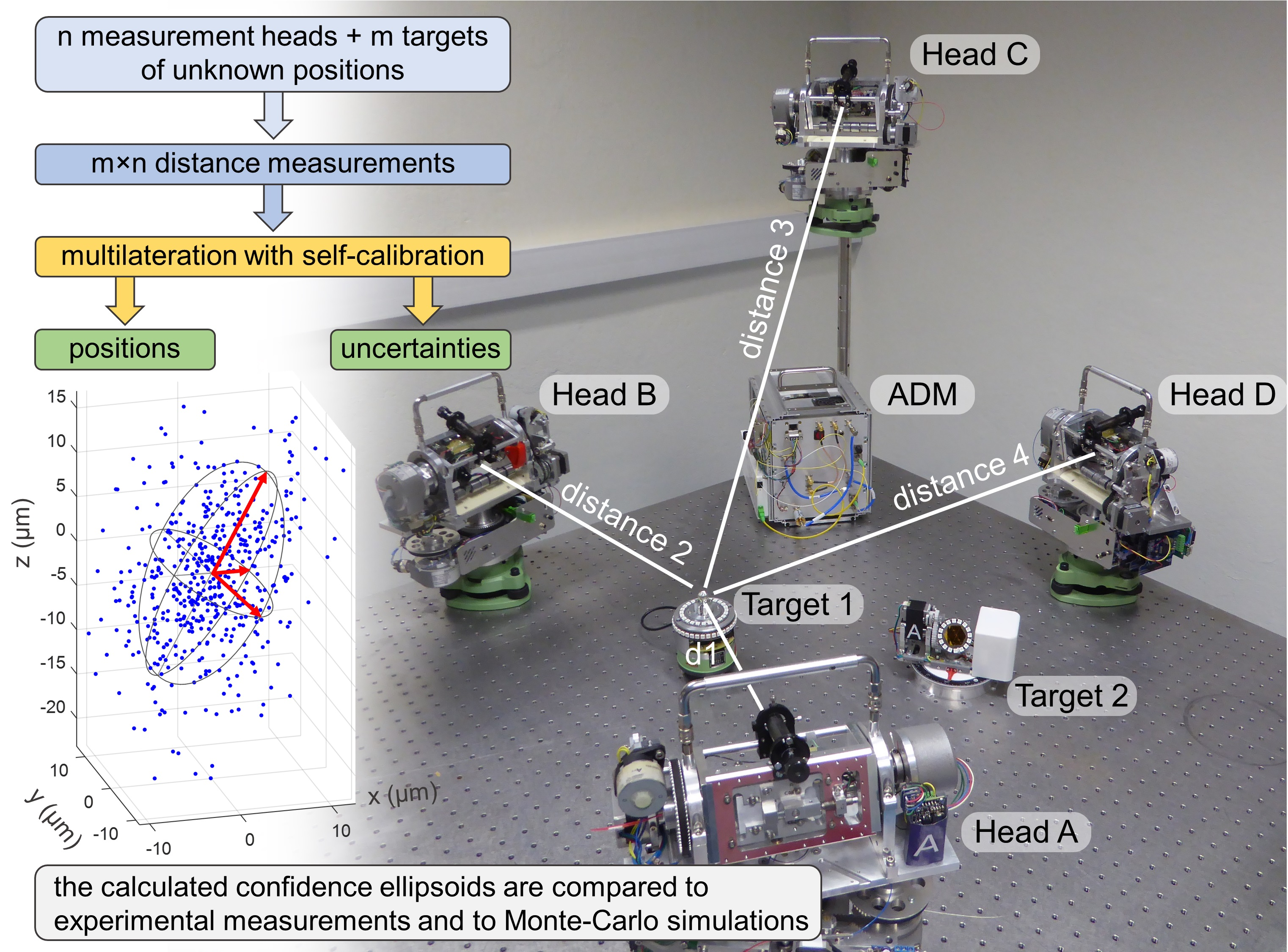
2.1. Determination of the Target Position

The classical multilateration problem consists of determining the coordinates of one target T from a set of several measurement heads H_i located at known coordinates [x_Hi, y_Hi, z_Hi], and performing distance measurements d_i up to this target. The true distance between one of these heads and the unknown target position [x_T, y_T, z_T] is:

$$d_i°\left(x_T,y_T,z_T\right)=\sqrt{{\left( x_T-x_{Hi} \right)}^2+{\left( y_T-y_{Hi} \right)}^2+{\left( z_T-z_{Hi} \right)}^2}$$

(2)

From a geometrical point of view, the target position is located at the intersection of spheres centered on the measurement heads and of radius equal to the distances measured by the absolute distance meter. At least four measurement heads are required to obtain a unique solution. Nevertheless, in practice, the use of three heads can be sufficient: this leads to two solutions, but the ambiguity can be resolved with basic assumptions based on the application.

In other words, with algebraic terms, when the number of distance measurements is higher than the number of unknown variables to estimate (i.e., the three coordinates of the target), the localization problem can be solved. However, due to uncertainties associated to the distance measurements, the target position should be determined using a non-linear least-squares approach where the optimal coordinates [x_T, y_T, z_T] of the target T are those which minimize the following quantity:

$$\mathit{cost} \mathit{function}={\displaystyle \sum }_{ i=1}^{ m} {\left( d_i\left(x_T,y_T,z_T\right)-‖H_i-T‖\right)}^2$$

(3)

where ‖.‖ denotes the Euclidian norm of a vector and d_i(x_T, y_T, z_T) is the distance measured between the measurement head H_i and the target T. It is assumed that the measured distances are affected by an additive random zero-mean Gaussian noise of known covariance.

To solve the multilateration problem of Equation (3), an iterative Gauss–Newton algorithm has been adopted. Indeed, Equation (3) is non-linear with unknown parameters vector [x_T, y_T, z_T]. Linearizing it via a Taylor series expansion is one possible solution. Thus, an estimate of the coordinates of the target is first assumed, T₀ = [x_T0, y_T0, z_T0]. Then, from this estimate, the approximation of the measured distances d_i(x_T, y_T, z_T) is obtained using a first-order Taylor expansion:

$$\begin{array}{c}{d}_i\left(x_T,y_T,z_T\right)\hfill \\ \approx d_i\left(x_{T0},y_{T0},z_{T0}\right)+{\left.\frac{\partial d_i\left(x_T,y_T,z_T\right)}{\partial x_T}\right|}_{\begin{array}{c}{x}_{T0}\\ y_{T0}\\ z_{T0}\end{array}}\Delta x+{\left.\frac{\partial d_i\left(x_T,y_T,z_T\right)}{\partial y_T}\right|}_{\begin{array}{c}{x}_{T0}\\ y_{T0}\\ z_{T0}\end{array}}\Delta y+{\left.\frac{\partial d_i\left(x_T,y_T,z_T\right)}{\partial z_T}\right|}_{\begin{array}{c}{x}_{T0}\\ y_{T0}\\ z_{T0}\end{array}}\Delta z\hfill \\ \approx d_i\left(x_{T0},y_{T0},z_{T0}\right)+{\left.\frac{x_T-x_{Hi}}{d_i\left(x_T,y_T,z_T\right)}\right|}_{\begin{array}{c}{x}_{T0}\\ y_{T0}\\ z_{T0}\end{array}}\Delta x+{\left.\frac{y_T-y_{Hi}}{d_i\left(x_T,y_T,z_T\right)}\right|}_{\begin{array}{c}{x}_{T0}\\ y_{T0}\\ z_{T0}\end{array}}\Delta y+{\left.\frac{z_T-z_{Hi}}{d_i\left(x_T,y_T,z_T\right)}\right|}_{\begin{array}{c}{x}_{T0}\\ y_{T0}\\ z_{T0}\end{array}}\Delta z\hfill \\ \approx d_i\left(x_{T0},y_{T0},z_{T0}\right)+\frac{x_{T0}-x_i}{d_i\left(x_{T0},y_{T0},z_{T0}\right)}\Delta x+\frac{y_{T0}-y_i}{d_i\left(x_{T0},y_{T0},z_{T0}\right)}\Delta y+\frac{z_{T0}-z_i}{d_i\left(x_{T0},y_{T0},z_{T0}\right)}\Delta z\hfill \end{array}$$

(4)

with Δx = (x_T − x_T0), and similarly for Δy and Δz. Arranged in a matrix form, this gives:

$$\Delta d=J\times \left[\begin{array}{c}\Delta x\\ \Delta y\\ \Delta z\end{array}\right]$$

(5)

where ∆d is a column vector equal to the differences between the measured distances and the approximate ones:

$$\Delta d_i=d_i\left(x_T,y_T,z_T\right)-d_i\left(x_{T0},y_{T0},z_{T0}\right)$$

(6)

and where J is a n × 3 matrix whose row numbered i corresponds to the derivatives:

$$J_i=\left[ \begin{array}{ccc}\frac{x_{T0}-x_{Hi}}{d_i\left(x_{T0},y_{T0},z_{T0}\right)}& \frac{y_{T0}-y_{Hi}}{d_i\left(x_{T0},y_{T0},z_{T0}\right)}& \frac{z_{T0}-z_{Hi}}{d_i\left(x_{T0},y_{T0},z_{T0}\right)}\end{array} \right]$$

(7)

The error correction vector is then calculated as follows:

$$\left[ \begin{array}{c}\Delta x\\ \Delta y\\ \Delta z\end{array} \right]={\left(J^{T}J\right)}^{-1}\times J^T\times \Delta d$$

(8)

From this result, the estimate of the target coordinates T₀ is updated. In practice, this Gauss–Newton recursive process is repeated until the coordinates of the error correction vector are small enough.

$$T_{0 updated}=\left[ \begin{array}{c}{x}_{T0}+\Delta x\\ y_{T0}+\Delta y\\ z_{T0}+\Delta z\end{array} \right]$$

(9)

This method is simple to implement and provide accurate results. Nevertheless, it is not the only way to resolve a multilateration problem with measurement head positions perfectly known, other approaches are proposed in the literature [16,17,18,19].

Lastly, to take into account the potential different uncertainties on the measured distances, a weighted least-squares method can be implemented by introducing the weight matrix W = cov(d)⁻¹. In such a case, the error correction vector is calculated as follows (Gauss-Markov theorem [20]):

$$\left[ \begin{array}{c}\Delta x\\ \Delta y\\ \Delta z\end{array} \right]={\left(J^T W J\right)}^{-1}\times J^T\times W\times \Delta d$$

(10)

The covariance matrix of the measured distances, cov(d), is a m × m square matrix of indices a (rows) and b (columns) which depends on the variances of the distances d_i measured by the heads i:

$$cov\left(d\right)=\left\{\begin{array}{ll}{ }_{d_i}{}^2\hfill & \mathrm{for} a=b \mathrm{and} i=a\hfill \\ 0\hfill & \mathrm{otherwise}\hfill \end{array}\right.$$

(11)

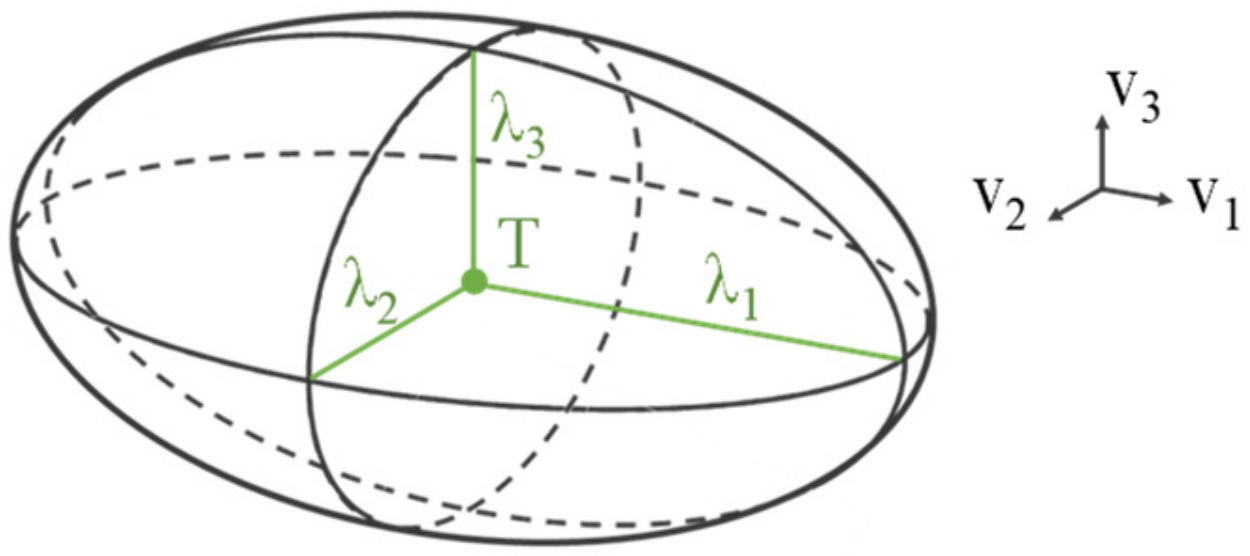
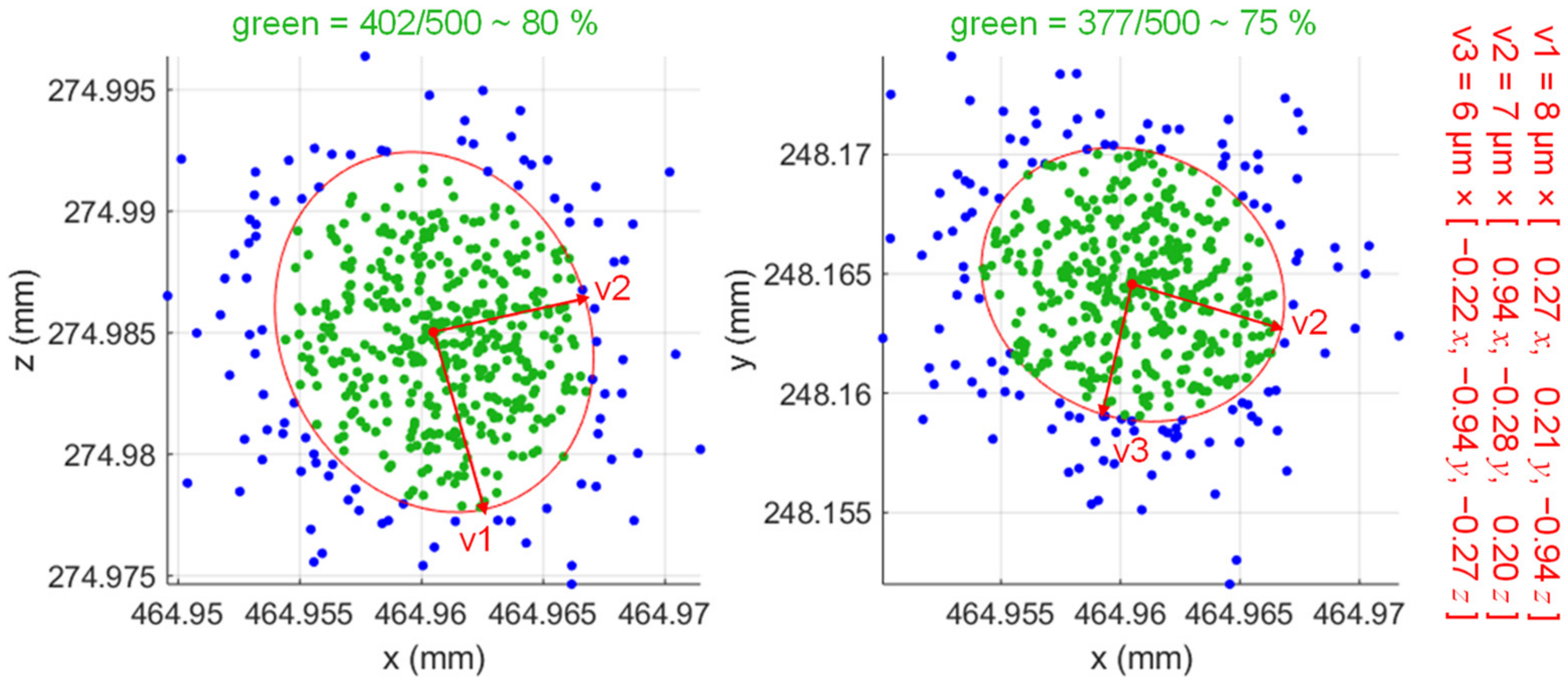
2.2. Uncertainty Assessment and Confidence Ellipsoid

To establish how sensitive is the estimate of a target position with respect to the inaccuracy of the distance measurements, but also with respect to the geometric arrangement of the system, the Cramér-Rao Lower bound (CRLB) is widely used. This is a well-known result of the mathematical statistics that gives a lower bound of the covariance of the estimated target position T [21,22].

$$cov\left(T\right)\ge CRLB$$

(12)

In the case of an efficient and unbiased localization algorithm (called estimator in estimation theory), the lower bound will be reached, which is the case for the localization algorithm presented in the preceding part and for our experiments where the measured distances are characterized by a zero-mean Gaussian noise.

In practice, this was determined from a first-order Taylor expansion of the measured distances. As shown in Formula (8), the residual error on the target position along the three axes, ∆T = [∆x ∆y ∆z]^T, can be expressed as a function of the differences ∆d between the measured distances and the approximate ones. Thus, using the law of propagation of uncertainty, it can be written:

$$cov\left(T\right)={\left(J^{T}J\right)}^{-1} J^T cov\left(d\right) J {\left(J^{T}J\right)}^{-1}$$

(13)

with cov(T) = cov(∆T), and cov(d) defined in Formula (11).

The uncertainty σ_T on the target position, for a confidence region of one-sigma (i.e., 68%), can then be deduced as follows:

$${\sigma }_T=\sqrt{Trace\left(cov\left(T\right)\right)}$$

(14)

where Trace is an operator that returns the sum of the diagonal elements of the matrix.

The covariance of T is a symmetric matrix. Therefore, there are orthonormal vectors v₁, v₂ and v₃ in which cov(T) is a diagonal matrix, called Q. These vectors are the eigenvectors of cov(T), with corresponding eigenvalues λ_j. v₁ corresponds to the direction with the highest uncertainty, while v₃ corresponds to the direction with the lowest uncertainty.

$$Q=\left[\begin{array}{ccc}{{𝜆}_1}^2& 0& 0\\ 0& {{𝜆}_2}^2& 0\\ 0& 0& {{𝜆}_3}^2\end{array}\right]$$

(15)

By this way, we define the confidence ellipsoid depicted in Figure 2 whose axes are in the direction of the eigenvectors and the corresponding eigenvalues give half the length of the axes. These parameters are obtained by proceeding to a singular value decomposition (SVD) of cov(T).

This confidence ellipsoid approximates a confidence region of 20% around a measured target position in space. In general, confidence regions of 68%, 95% and 99% are used. To obtain them, scaling factor of, respectively, 1.88, 2.79 and 3.58 are applied to move towards a trivariate error distribution under the assumption that the uncertainties follow Gaussian distributions [23,24].

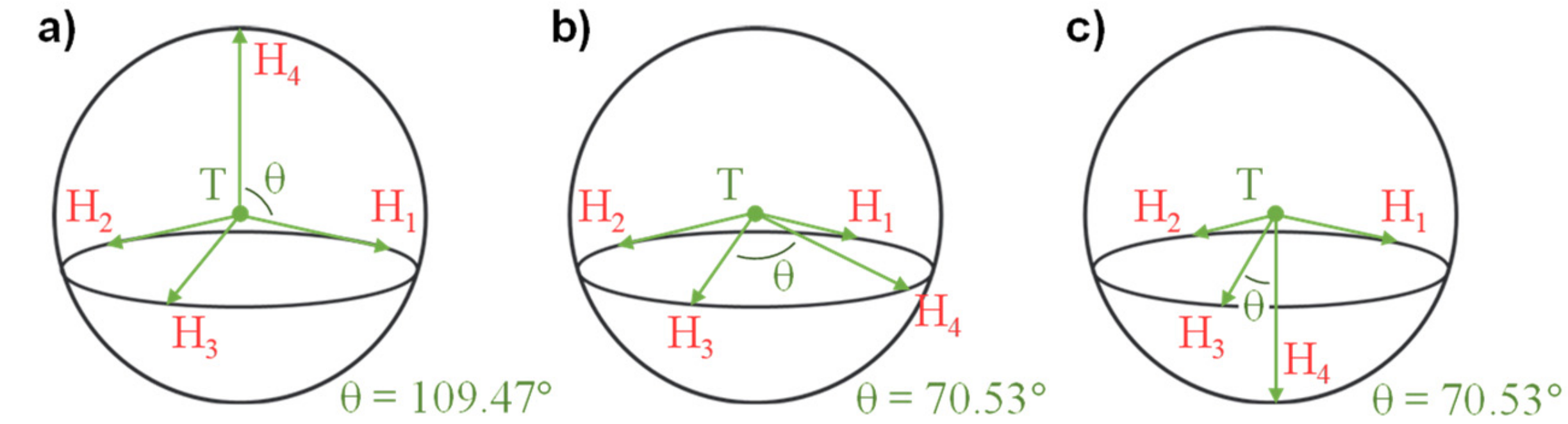
2.3. Best Arrangements for Multilateration with 4 Heads

The optimal arrangement that minimized the uncertainty for a configuration with four measurement heads has been studied in [25]. There are three possible arrangements. First, in Figure 3a, the geometry formed by the four heads can be a regular tetrahedron with the target located at the centre. Then, in Figure 3b, the four heads can be distributed regularly on a circle with an angle between two adjacent head-target vectors equal to 70.53°. Lastly, in Figure 3c, the geometry formed by the four heads can be an isosceles tetrahedron with the target located slightly outside.

In these three cases, the uncertainty is equal to its minimum value, i.e., k × σ_d/sqrt(m) = 1.5 × σ_d, with k = 3 the number of the dimensional space, m = 4 the number of measurement heads, and σ_d the uncertainty on the measured distances [26]. This means that our coordinate measurement system, with uncertainties on the measured distances around 5 µm and assuming the positions of the measurement heads known and error free, will not have an uncertainty of less than 7.5 µm.

3. Multilateration in the Presence of Uncertainties on the Measurement Head Positions

3.1. Determination of the Target Position

Up to now, only two influencing factors have been considered: the distance errors and the geometry. In this part, the errors made on the positions of the measurement heads are also considered. To resolve it, we have adopted the localization method presented in [27].

The true distances d_i° and the true coordinates of the measurement heads H_i° are affected by additive random zero-mean Gaussian noises of known covariance. Let n_d = [n_d1 n_d2 … n_dm]^T be the first error vector and n_H = [n_xH1 n_yH1 n_zH1 … n_zHm]^T be the second one.

$$\left\{\begin{array}{c}{d}_i=d_i°+n_{d_i}\\ x_{H_i}=x_{H_i}°+n_{x_{H_i}}\\ y_{H_i}=y_{H_i}°+n_{y_{H_i}}\\ z_{H_i}=z_{H_i}°+n_{z_{H_i}}\end{array}\right.$$

(16)

The unknown true target position T° = [x_T°, y_T°, z_T°] should so satisfy a system of m equations described in the following form:

$$\begin{array}{cc}\hfill {\left(d_i-n_{di}\right)}^2=& {\left(x_T°-\left(x_{Hi}-n_{xHi}\right)\right)}^2+\cdots \hfill \\ \hfill & {\left(y_T°-\left(y_{Hi}-n_{yHi}\right)\right)}^2+{\left(z_T°-\left(z_{Hi}-n_{zHi}\right)\right)}^2\hfill \end{array}$$

(17)

When second order noise terms are ignored, we obtain m equations of the form:

$$\begin{array}{cc}\hfill {d_i}^2-2 d_i n_{di}=& \left(x_T°{}^2+y_T°{}^2+z_T°{}^2\right)-2 \left(x_T° x_{Hi}+y_T° y_{Hi}+z_T° z_{Hi}\right) \dots \hfill \\ \hfill & +2 \left(x_T° n_{xHi}+y_T° n_{yHi}+z_T° n_{zHi}\right)+\left(x_{Hi}{}^2+y_{Hi}{}^2+z_{Hi}{}^2\right)\dots \hfill \\ \hfill & -2 \left(x_{Hi} n_{xHi}+y_{Hi} n_{yHi}+z_{Hi} n_{zHi}\right)\hfill \end{array}$$

(18)

Let A be a m × 4 matrix containing the position information of the measurement heads and B a column vector:

$$A=\left[ \begin{array}{cccc}1& -2 x_{H1}& -2 y_{H1}& -2 z_{H1}\\ 1& -2 x_{H2}& -2 y_{H2}& -2 z_{H2}\\ ⋮& ⋮& ⋮& ⋮\\ 1& -2 x_{Hm}& -2 y_{Hm}& -2 z_{Hm}\end{array} \right]$$

(19)

$$B=\left[\begin{array}{c} d_1{}^2-\left(x_{H1}{}^2+y_{H1}{}^2+z_{H1}{}^2\right) \\ d_2{}^2-\left(x_{H2}{}^2+y_{H2}{}^2+z_{H2}{}^2\right) \\ ⋮ \\ d_{nm}{}^2-\left(x_{Hm}{}^2+y_{Hm}{}^2+z_{Hm}{}^2\right) \end{array}\right]$$

(20)

Therefore, the system of Equation (18) can be written in this form:

$$B=A\times \left[\begin{array}{c}{x}_T{°}^2+y_T{°}^2+z_T{°}^2\\ x_T°\\ y_T°\\ z_T°\end{array}\right]+e_1$$

(21)

with e₁ the error matrix:

$$\begin{array}{cc}\hfill e_1=& 2\times \left[\begin{array}{cccc} d_1& 0& & 0\\ 0& d_2& & 0\\ & & \ddots & ⋮\\ 0& 0& \dots & d_m\end{array}\right]n_d+2\times \dots \hfill \\ \hfill & \left[\begin{array}{ccccccc}{x}_T°-x_{H1}& y_T°-y_{H1}& z_T°-z_{H1}& & & 0_{1\times 3}& \\ & ⋮& & \ddots & & ⋮& \\ & 0_{1\times 3}& & & x_T°-x_{Hm}& y_T°-y_{Hm}& z_T°-z_{Hm}\end{array}\right] n_H\hfill \\ \hfill =& N_d\times n_d+N_H\times n_H\hfill \end{array}$$

(22)

The system of Equation (21) is non-linear with respect to the coordinates of the target x_T°, y_T° and z_T°. However, if we assume that x_T°² + y_T°² + z_T°² is independent of the variables x_T°, y_T° and z_T°, which is mathematically non-rigorous, the system can be resolved, but at the cost of inaccurate results. Let T₁ be a first approximation of the result of this system of equations:

$$T_1=\left[\begin{array}{c}{x}_T{}^2+y_T{}^2+z_T{}^2\\ x_T\\ y_T\\ z_T\end{array}\right]={\left(A^{T}A\right)}^{-1}\times A^T\times B$$

(23)

In practice, to take into account the error e₁, a weighted least-squares method is implemented with the weight matrix W₁ = E[e₁ e₁^T]⁻¹ (Gauss-Markov theorem [20]):

$$T_1=\left[\begin{array}{c}{x}_T{}^2+y_T{}^2+z_T{}^2\\ x_T\\ y_T\\ z_T\end{array}\right]={\left(A^T{W}_{1}A\right)}^{-1}{A}^T{W}_1\times B$$

(24)

with:

$$W_1={\left(N_d Cov\left(d\right) N_d{}^T+N_H Cov\left(H\right) N_H{}^T\right)}^{-1}$$

(25)

The calculation of the weight matrix W₁, and more precisely N_H, requires the knowledge of the true target position T°. However, the latter can be replaced by a first estimate of the target using Equation (23) or applying the algorithm presented previously in Section 2.1.

For a better estimate, a second step is then performed to determine a second approximation of the true value T°. Let first ΔT be the error on the approximation made previously:

$$\begin{array}{cc}\hfill T_1& =\left[\begin{array}{c}{x}_T{}^2+y_T{}^2+z_T{}^2\\ x_T\\ y_T\\ z_T\end{array}\right]\hfill \\ \hfill & =\left[\begin{array}{c}{x}_T{°}^2+y_T{°}^2+z_T{°}^2\\ x_T°\\ y_T°\\ z_T°\end{array}\right]+\left[\begin{array}{c}\Delta x_T{}^2+2x_T°\Delta x_T+\Delta y_T{}^2+2y_T°\Delta y_T+\Delta Z_T{}^2+2z_T°\Delta z_T\\ \Delta x_T\\ \Delta y_T\\ \Delta z_T\end{array}\right]\hfill \end{array}$$

(26)

A new matrix D is then defined from the square of the coordinates of T₁.

$$D=\left[\begin{array}{c}{x}_T{}^2+y_T{}^2+z_T{}^2\\ x_T{}^2\\ y_T{}^2\\ z_T{}^2\end{array}\right]=\left[\begin{array}{c}{T}_1\left(1\right)\\ T_1{\left(2\right)}^2\\ T_1{\left(3\right)}^2\\ T_1{\left(4\right)}^2\end{array}\right]$$

(27)

From the Formula (26), and ignoring the second order noises, D can also be expressed as follows:

$$\begin{array}{cc}\hfill D& =\left[\begin{array}{ccc}1& 1& 1\\ 1& 0& 0\\ 0& 1& 0\\ 0& 0& 1\end{array}\right]\times \left[\begin{array}{c}{x}_T{°}^2\\ y_T{°}^2\\ z_T{°}^2\end{array}\right]+\left[\begin{array}{cccc}1& 0& 0& 0\\ 0& 2x_T°& 0& 0\\ 0& 0& 2y_T°& 0\\ 0& 0& 0& 2z_T°\end{array}\right]\times \left[\begin{array}{c}\Delta x_T\\ \Delta y_T\\ \Delta z_T\end{array}\right]\hfill \\ \hfill & =C\times \left[\begin{array}{c}{x}_T{°}^2\\ y_T{°}^2\\ z_T{°}^2\end{array}\right]+N_T\times \Delta T\hfill \end{array}$$

(28)

Thus, the square of the true value of T° can be approximated as:

$$T_2=\left[\begin{array}{c}{x}_T{°}^2\\ y_T{°}^2\\ z_T{°}^2\end{array}\right]={\left(C^{T}C\right)}^{-1}\times C^T\times D$$

(29)

In practice, the error e₂ = N_T × ΔT is taken into account by using the weight matrix W₂ = E[e₂e₂^T]⁻¹:

$$T_2={\left(C^T{W}_{2}C\right)}^{-1}{C}^T{W}_2\times D$$

(30)

with:

$$W_2={\left(N_T Cov{\left(T_1\right)}^{-1} N_T{}^T\right)}^{-1}={\left(N_T{}^T\right)}^{-1} {\left(A^T W_1 A\right)}^{-1} N_T{}^{-1}$$

(31)

To calculate the weight matrix W₂, and more precisely N_T, the target values from the first estimation T₁ are used instead of the values of T°.

3.2. Uncertainty Assessment

As explained in Section 2, it is of interest to know the Cramér-Rao Lower Bound of the estimated parameters. Let θ° be the vector of the unknown parameters. It is composed of the exact values of the coordinates of the target and of the m measurement heads: θ° = [x_T° y_T° z_T° x_H1° y_H1° z_H1° x_H2° y_H2° z_H2° … x_Hm° y_Hm° z_Hm°]^T. The distances d_i° are not part of this vector as they are already included since d_i° = f(x_T°, y_T°, z_T°, x_Hi°, y_Hi°, z_Hi°).

In estimation theory, it is stated that the covariance of the estimate of θ°, noted cov(θ), is at least as high as the inverse of the Fisher information matrix, denoted by FIM. In other words, the CRLB is the inverse of the FIM.

$$cov\left(\theta \right)\ge FIM{\left(\theta °\right)}^{-1}$$

(32)

The FIM represents the information provided by the observation λ (i.e., the measurements) about the unknown parameter vector θ°. The observation vector λ is composed of the measured distances and of the estimated coordinates of the m measurement heads: λ = [d₁ … d_m x_H1 y_H1 z_H1 … z_Hm]^T. Each value of this observation vector has an associated uncertainty with a known distribution.

Let l be the log-likelihood function of θ° given λ, noted l(θ°| λ). Therefore:

$$FI{M}_{a,b}\left(\theta °\right)=-E\left[\frac{{\partial }^2}{\partial {\theta }_a° \partial {\theta }_b°}l\left(\theta °|\lambda \right)\right]=\left[\begin{array}{cc}X& Y\\ Y^T& Z\end{array}\right]$$

(33)

with X the second-order partial derivatives of the log-likelihood function l(θ°| λ) with respect to the true coordinates of the target, Z the second-order partial derivatives of l(θ°| λ) with respect to the true coordinates of the four measurement heads, Y is the partial derivatives of l(θ°| λ) with respect to the true coordinates of both, the target and the m measurement heads. The FIM is a square matrix of indexes a and b, and of size 3 (m + 1) × 3 (m + 1).

Let f be the probability density function (PDF) of the values of the observation vector. For instance, for the first coordinate of the measurement head i, x_Hi, described by a Gaussian distribution:

$$f_{xHi}\left(x_{Hi}\right)=\frac{1}{\sqrt{ 2\pi {\sigma }_{xHi}{}^2 }}{e}^{-\frac{{\left(x_{Hi}-x_{Hi}°\right)}^2}{ 2{\sigma }_{xHi}{}^2}}$$

(34)

This function is so parametrized by θ°. In the same manner, similar formulas are obtained for the other coordinates of the four measurement heads of the observation vector λ. Besides, for the distances d_i:

$$\begin{array}{cc}\hfill f_{di}\left(d_i\right)& =\frac{1}{\sqrt{ 2\pi {\sigma }_{di}{}^2 }}{e}^{-\frac{{\left(d_i-\sqrt{(x_{Hi}°-x_T°)²+(y_{Hi}°-y_T°)²+(z_{Hi}°-z_T°)²}\right)}^2}{ 2{\sigma }_{di}{}^2}}\hfill \\ \hfill & =\frac{1}{\sqrt{ 2\pi {\sigma }_{di}{}^2 }}{e}^{-\frac{{\left(d_i-d_i°\right)}^2}{ 2{\sigma }_{di}{}^2}}\hfill \end{array}$$

(35)

The log-likelihood function can then be developed as follows since the variables of the observation vector are statistically independent of each other [28]:

$$\begin{array}{ccc}\hfill l\left(\theta °|\lambda \right)& \hfill =\hfill & {\displaystyle {\displaystyle \sum }_{i=1}^m}\ln f_{di}\left(d_i;\theta °\right)+{\displaystyle {\displaystyle \sum }_{i=1}^m}\ln f_{xHi}\left(x_{Hi};\theta °\right)+{\displaystyle {\displaystyle \sum }_{i=1}^m}\ln f_{yHi}\left(y_{Hi};\theta °\right)\dots \hfill \\ \hfill & \hfill \hfill & +{\displaystyle {\displaystyle \sum }_{i=1}^m}\ln f_{zHi}\left(z_{Hi};\theta °\right)\hfill \\ \hfill & \hfill =\hfill & {\displaystyle {\displaystyle \sum }_{i=1}^m}\ln f_{di}\left(d_i; x_T°,y_T°,z_T°,x_{Hi}°,y_{Hi}°,z_{Hi}°\right)+{\displaystyle {\displaystyle \sum }_{i=1}^m}\ln f_{xHi}\left(x_{Hi}; x_{Hi}°\right)\dots \hfill \\ \hfill & \hfill \hfill & +{\displaystyle {\displaystyle \sum }_{i=1}^m}\ln f_{yHi}\left(y_{Hi}; y_{Hi}°\right)+{\displaystyle {\displaystyle \sum }_{i=1}^m}\ln f_{zHi}\left(z_{Hi}; z_{Hi}°\right)\hfill \end{array}$$

(36)

From this, the calculation of the FIM can be performed. After an onerous calculation, not detailed in this paper, the three block matrices X, Y and Z are equal to [27,29]:

$$\begin{array}{c}X=M_d{}^T\times cov{\left(d\right)}^{-1}\times M_d\hfill \\ Y=M_d{}^T\times cov{\left(d\right)}^{-1}\times M_H\hfill \\ Z=M_H{}^T\times cov{\left(d\right)}^{-1}\times M_H+cov{\left(H\right)}^{-1}\hfill \end{array}$$

(37)

with cov(d) defined in Formula (11) and:

$$cov\left(H\right)=\mathrm{diag}( [{{\sigma }_{x{H}_1}}^2,{{\sigma }_{y{H}_1}}^2,{{\sigma }_{z{H}_1}}^2, \dots , {{\sigma }_{x{H}_1}}^2] ).$$

(38)

$$M_d=\frac{\partial d}{\partial T°}=\left[\begin{array}{ccc}\frac{x_T°-x_{H1}°}{d_1}& \frac{y_T°-y_{H1}°}{d_1}& \frac{z_T°-z_{H1}°}{d_1}\\ ⋮& ⋮& ⋮\\ ⋮& ⋮& ⋮\\ \frac{x_T°-x_{H4}°}{d_4}& \frac{y_T°-y_{H4}°}{d_4}& \frac{z_T°-z_{H4}°}{d_4}\end{array}\right]$$

(39)

$$M_H=\frac{\partial d}{\partial H°}=\left[\begin{array}{ccc}\begin{array}{ccc}\frac{x_T°-x_{H1}°}{d_1}& \frac{y_T°-y_{H1}°}{d_1}& \frac{z_T°-z_{H1}°}{d_1}\end{array}& 0& 0\\ \begin{array}{ccc} 0 & 0 & 0 \end{array}& \frac{x_T°-x_{H2}°}{d_2}& ⋮\\ ⋮& ⋮& ⋮\\ 0& 0& \begin{array}{ccc}\frac{x_T°-x_{H4}°}{d_4}& \frac{y_T°-y_{H4}°}{d_4}& \frac{z_T°-z_{H4}°}{d_4}\end{array}\end{array}\right]$$

(40)

At the end, the CRLB of the target location corresponds to the upper left 3 × 3 submatrix of the inverse of the FIM. As previously, by proceeding to a singular value decomposition of this matrix, the confidence ellipsoid of the target can be obtained.

4. Multilateration with Self-Calibration

4.1. Determination of the Targets and Head Positions

In a multilateration technique with self-calibration, the measurement heads are located at unknown positions. However, by performing distance measurements for several target positions, a system of equations with more observations than unknowns is created. Thus, the coordinates of each target position, but also the coordinates of the measurement heads can be determined.

The multilateration algorithm with self-calibration requires initial values sufficiently accurate for the target and head positions [30]. For that purpose, in our system, the n positions of the targets are determined with an accuracy around 1 mm from the measurements of a single head, in the same way as a laser tracker. Indeed, each measurement head also records its two orthogonal angles (horizontal and vertical), thanks to angle encoders of around 400 µrad of resolution. Thus, in a cartesian system, the rough estimate of the position of a target j is:

$$x_j=d_{i,j}\times \sin {\phi }_i\cos {\theta }_i, y_j=d_{i,j}\times \sin {\phi }_i\sin {\theta }_i, z_j=d_{i,j}\times \cos {\phi }_i$$

(41)

with d_i,j the distances measured by the measurement head i (positive values), θ_i and φ_i the azimuth and elevation angles of this head (in radians, θ_i between 0 and 2π and φ_i between –π/2 and +π/2). This corresponds to the standard transformation from spherical to Cartesian coordinates.

In practice, the results from several heads are combined to mitigates the errors. To this end, a registration step based on Horn’s quaternion-based method is performed to express the different results in a unique system of coordinates. This consists of finding rotation matrices and translation vectors that best match one collection of target coordinates to another in a least-squares sense. Once that is carried out, a fusion algorithm is applied [23]. Lastly, when the initial values of the target positions have been determined, the initial values of the measurement head positions are calculated using the multilateration algorithm presented in Section 2.

At this step, the heads and targets are referenced in a new system of coordinates where one head defines the origin, a second one defines the x axis, and a last one defines the xOy plane. An example is provided in Equation (43). This is an arbitrary choice to fix the orientation of the coordinate system, but at the end, the positions of the heads and of the targets could be transformed into any coordinate system, thanks to a translation and rotations.

$$\begin{array}{c}\left[x_1,y_1,z_1\right]=\left[ 0 , 0 , 0 \right]\\ \left[x_2,y_2,z_2\right]=\left[x_2,0 , 0 \right]\\ \left[x_3,y_3,z_3\right]=\left[x_3,y_3,0\right]\end{array}$$

(42)

The coordinates x₂, x₃, y₃ and those of the other measurement heads must now be refined from their initial values. To do this, the following cost function is minimized:

$$cost function={\displaystyle \sum }_{i, j}{\left(d_{i,j}{}^2-{‖H_i-T_j\left(H_i, d_{i,j}\right)‖}^2\right)}^2$$

(43)

where the unknown inputs are the coordinates of the heads, reduced by 6 since some of them have been fixed to zero. For a given set of inputs H_i, the coordinates of the target positions T_j are calculated from the measured distances by using the multilateration algorithm presented in Section 2.

From a geometrical point of view, minimizing the cost function in Formula (43) is like looking for the radical center of four spheres, i.e., minimization of the sum of the squares of the power of the point T_j with respect to a sphere of center H_i and radius d_i,j [31].

In practice, a Levenberg–Marquardt method has been adopted to minimize the cost function. It is an algorithm for solving the non-linear least-squares problems. Like the Gauss–Newton method, it proceeds iteratively, and uses the Jacobian to define an error correction vector. However, it has the advantage of offering a better stability against the rank-deficiency of the Jacobian matrix [32].

When the cost function is minimized, and so the coordinates of the heads determined, the uncertainties on these coordinates are determined. By this way, the problem is basically the same as the one presented in Section 3: A multilateration system where the positions of the heads and their uncertainties are known.

4.2. Uncertainty Assessment

For multilateration algorithm with self-calibration, the FIM (or CRLB) is not used to analytically determine the uncertainties of the coordinates since it is rank deficient due to the translational and rotational ambiguity in the self-calibration solution [33]. In other words, the FIM is not invertible. To solve this problem, we propose in this paper our own solution.

First, we impose constraints on the multilateration problem in Formula (43) to remove the ambiguity. In our case, this consists of studying each measurement head separately: for a given head, numbered k, the problem is simplified considering that the coordinates of the heads H_i are known, error-free when i ≠ k and noise corrupted only when i = k. An approximation of the uncertainties of the coordinates of the heads can then be calculated on the basis of the empirical study in [34], which presents a method to determine the covariance matrix of parameters estimated by non-linear least-squares. To this end, it is assumed that the distances between the different measurement heads and targets can be written as a mathematical function f:

$$f\left(\theta =H_k,d_{i,j},H_i\right)=‖H_i-T_j\left(d_{i,j},H_i\right)‖$$

(44)

with the target positions T_j determined from the classical multilateration algorithm presented in Section 2 using the measured distances d_i,j and the coordinates [x_Hi, y_Hi, z_Hi] determined in Section 4.1.

The measured distances d_i,j are the response variables, while the positions of both targets T_j and heads H_i (with i ≠ k) are the predictor variables. The parameter to estimate is here θ°, the true but unknown coordinates of H_k. At the end, the measured distances d_i,j can therefore be modelled as follows:

$$d_{i,j}=f\left(\theta °,T_j,H_i\right)+e_{i,j}$$

(45)

with e_i,j random errors between the measured distances and the true ones. These errors are assumed independent and Gaussian distributed of mean equal to zero. According to [34], the covariance matrix of the estimated coordinates θ can be approximated from the Jacobian of f at the position θ = [x_Hk, y_Hk, z_Hk].

$$cov\left(\theta =H_k\right)=s^2\times {\left(J{\left(H_k\right)}^{T}J\left(H_k\right)\right)}^{-1}$$

(46)

where s is the estimated residual variance of f at position H_k:

$$s^2=\frac{1}{m\times n-p}\times {\displaystyle \sum }_{i=1}^m {\displaystyle \sum }_{j=1}^n{\left(d_{i,j}-f\left(H_k\right)\right)}^2$$

(47)

with p is the length of vector θ, i.e., p = 3.

The Jacobian matrix of f at position H_k describes how small changes into the coordinates of the head H_k will modify the distances derived from that position.

$$J\left(H_k\right)=\left[\begin{array}{ccc}{\left.\frac{\partial f\left(\theta \right) }{\partial x_{H_k}}\right|}_{H_k}& {\left.\frac{\partial f\left(\theta \right) }{\partial y_{H_k}}\right|}_{H_k}& {\left.\frac{\partial f\left(\theta \right) }{\partial z_{H_k}}\right|}_{H_k}\end{array}\right]$$

(48)

The calculation of the first-order partial derivatives of f(θ) appears particularly complex. It is in fact numerically differentiated at the estimated value H_k, for instance using the jacobianest function under Matlab^® [35].

In the proposed approach, each measurement head is treated independently. This approach is justified by the fact that if we consider in Formula (46) a function f of input variables the coordinates of all the measurement heads, the obtained covariance matrix would be rank-deficient with a rank equal to 3 × (m − 6).

As previously, from the covariance matrix of the estimated position θ, the confidence ellipsoid of each measurement head can be determined. This is now a multilateration problem with the uncertainties on both the distance measurements and the measurement head positions as previously presented in Section 3. It is therefore easy to also determine the uncertainties on the target positions.

Lastly, once the target positions and their uncertainties known, the uncertainties of the coordinates of the heads (but not their value) are refined using the method in Section 3.2.

Section 5 compares this analytical approach for computing the uncertainties, and so the confidence regions, from experimental results to Monte Carlo simulations.

4.3. Instrument Offsets

In the developed system, there are also instrument offsets to consider, one per measurement head. They are additive constants, expressed in meters, that compensate from delays in cables, electrical components and optical paths. Such corrections are required to have an electro-optical origin that corresponds to the zero of the instrument, and so to achieve absolute distance measurements between each measurement head and the targets.

$$d_{i,j absolute}=d_{i,j}+o_i$$

(49)

with o_i the offset linked to the head H_i.

In practice, these offsets can be determined, thanks to additional measurements on a small baseline composed of three pillars [36]: with the developed system, this calibration step provides offsets with uncertainties of a few micrometers.

Alternatively, these additional unknown variables can also be determined simultaneously to the multilateration measurement with self-calibration. To this end, the cost function in Formula (43) is modified as follows:

$$cost function={\displaystyle \sum }_{i,j}{\left({\left(d_{i,j}+o_i\right)}^2-{‖H_i-T_j\left(H_i, d_{i,j}+o_i\right)‖}^2\right)}^2$$

(50)

Once the offsets have been determined by using one of the two above methods, the measured distances are corrected. The offsets are assumed constant. As a consequence, the offset calibration of the developed coordinate measurement system can be performed just once. In practice, it is better to determine them occasionally because they can change with time due to, for instance, a temperature dependency.

If we assume that the measured distances were corrected from the offsets after a first calibration step: the offsets are known, but affected by an additive zero-mean Gaussian noise of known standard deviation. Thus, we can perform multilateration measurements with self-calibration as detailed in Section 4 by replacing the measured distances by the absolute distances calculated in Formula (49). In that case, the uncertainties on the absolute distances are calculated as follows:

$${{\sigma }_{d_{i,j} absolute}}^2={{\sigma }_{d_{i,j}}}^2+{{\sigma }_{o_i}}^2$$

(51)

In this paper, the uncertainty assessment of a multilateration measurement with a self-calibration that includes the offsets has not been considered. In such a case, with unknown offsets, it is like if the observations, i.e., the measured distances d_i,j, are corrupted by non-zero mean errors: the random errors e_i,j in Formula (45) include also the offset, they do not have therefore a zero mean value. The method proposed in Section 4.2 and based on the empirical study in [34] is simply not valid.

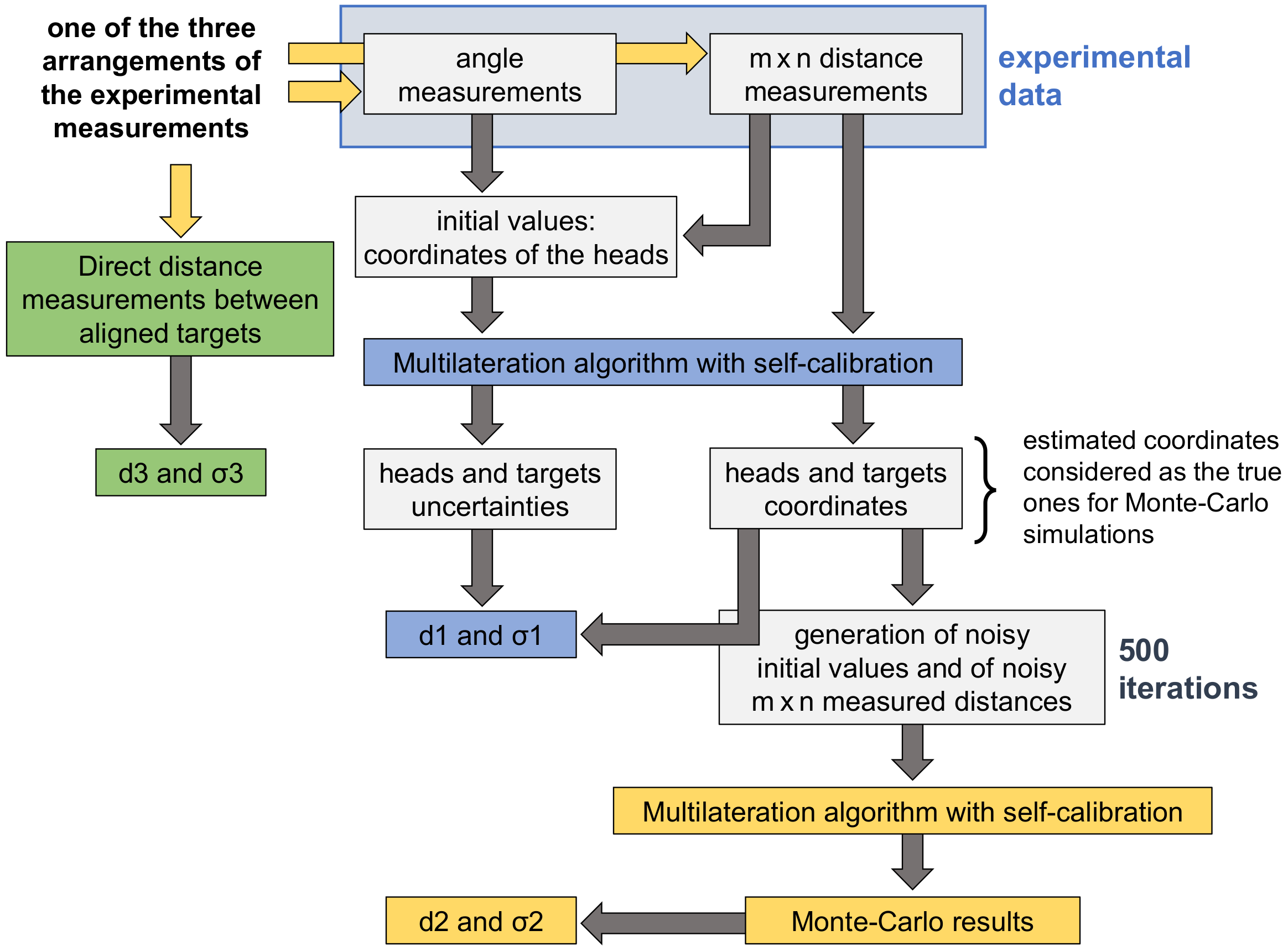
5. Experimental Results versus Monte-Carlo Simulations for Multilateration with Self-Calibration

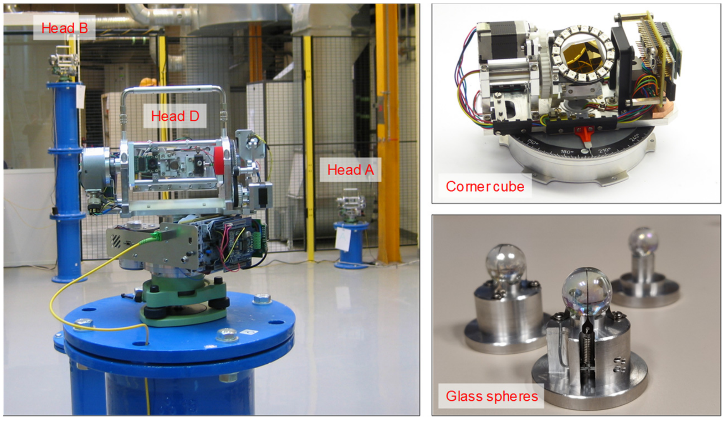
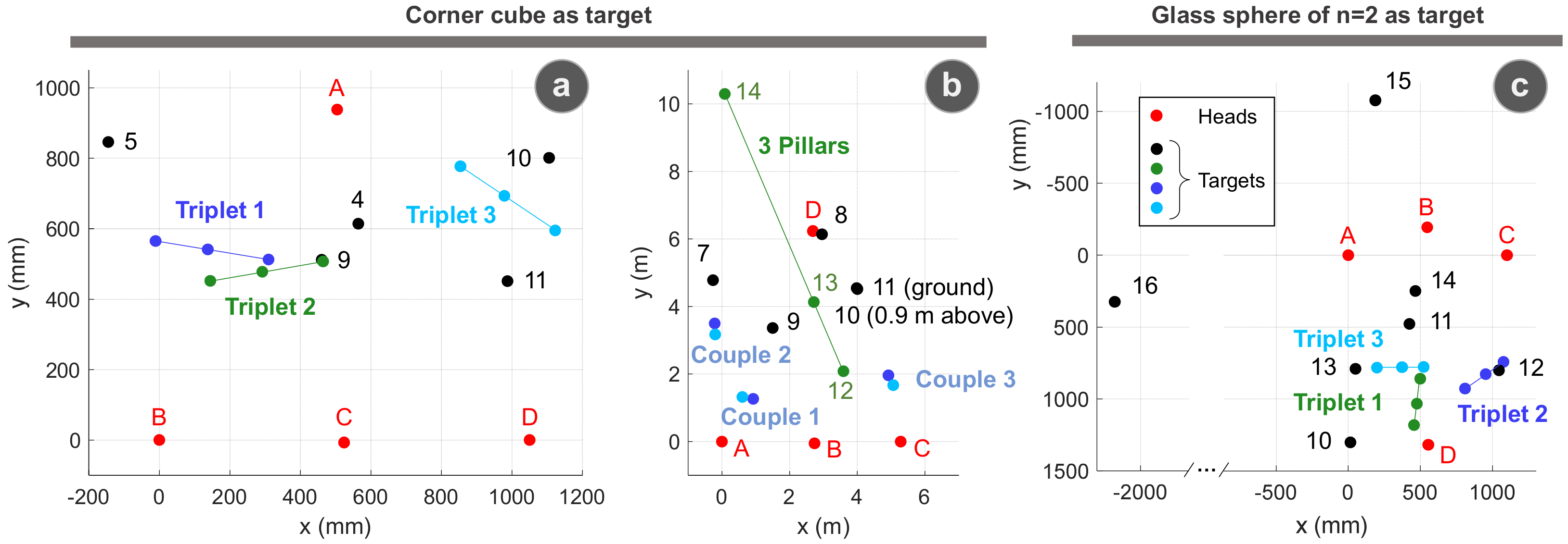
5.1. Experimental Results

To validate the approach developed in Section 4 that provides the confidence ellipsoids of the target and measurement head positions, three different experimental measurements have been performed:

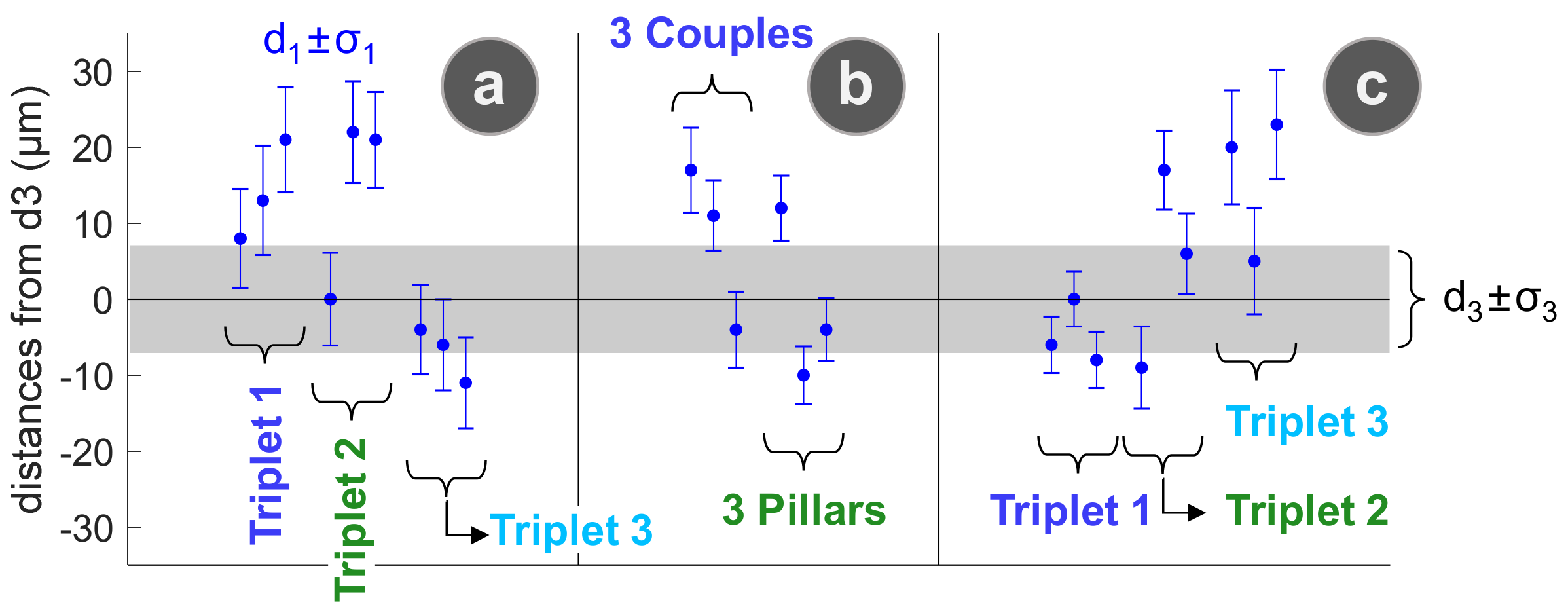
• The first case is a small volume of one cubic meter using a corner cube as target in 14 different positions.
• The second case is a large volume with distances up to 11.5 m and a corner cube in 14 different positions.
• The third case is a small volume of one cubic meter using a glass sphere of index n = 2 as target in 16 different positions.

Figure 4 depicts the layouts of the 4 measurement heads (identified by letters from A to D corresponding to heads H_i, with i from 1 to 4) and of the different target positions for these three experimental cases. The arrangements of the heads were always close to a regular tetrahedron in order to optimize the uncertainties (see Figure 3a), and the targets were preferably placed inside the volume formed by the heads, with the exception of specific cases for testing longer distances.

The uncertainty on the measured distances (at k = 1) has been assessed at 4.7 µm when the target is a corner cube [2] and at 4.3 µm when it is a glass sphere of index n = 2 [3]. These values include the contribution of the target uncertainty. When the target is a corner cube, the target can be oriented in any direction by means of a gimbal mechanism. Like any mechanical system, not perfectly machined and assembled, this gimbal mechanism induces errors on the geometric distances. These errors have been characterized, then minimized by adjusting the position of the corner cube into the gimbal mechanism. In addition, some systematic errors are corrected. At the end, they represent the main contribution to the uncertainty of the distance measurements with a value of 3.9 μm (k = 1, zero-mean Gaussian distributed [2]). When the target is a sphere visible from almost any angle, it does not require such a mechanism. In this case, the main contribution to the distance uncertainty comes from the random noise of 2.1 μm observed on the distance measurements. In fact, the random noise is lower when a corner cube is used and is equal to 0.8 µm. The bad reflectivity of the spheres and the beam deflection they induce increase the random noise. However, the uncertainty may be a little bit higher in practice due to the determination of the atmospheric parameters, especially in the large volume where a vertical temperature gradient of 1 °C was observed.

The multilateration algorithm with self-calibration described in Section 4.1 has been applied to the three experimental measurements to obtain the positions of both targets and measurement heads. However, it must be emphasized that in all these cases, the instrument offsets have been determined simultaneously to the multilateration process, which is the critical case where the uncertainty assessment has not been studied. The algorithm has always perfectly converged: the standard deviations on the difference between the distances measured by our absolute distance meter, and those deduced from the positions provided by the multilateration algorithm were always lower than 4 µm.

Then, from the uncertainty assessment described in Section 4.2, all the determined positions k (both heads and targets) have been characterized by a covariance matrix and an associated confidence ellipsoid. We have operated ignoring the instrument offsets, as if they had no impact. This approach should be seen as an approximation in the absence of any more reliable solution. The comparisons presented subsequently will assess the impact of this choice.

The uncertainty, expressed as a single-number indicator, has been calculated as follows:

$$\sigma \left(po{s}_k\right)=\sqrt{Trace\left(cov\left(po{s}_k\right)\right)}$$

(52)

To validate the experimental results, reference measurements are required. To address this issue, some distances between different target positions have been measured in a direct way by the absolute distance meter (it means without multilateration) and compared to the same distances when calculated from the target positions provided by the multilateration algorithm. For the small volumes, these points correspond to a triplet of aligned target positions mounted on a same breadboard, breadboard which has been displaced several times into the volume. For the large volume, these points correspond to a couple of target positions mounted on a same breadboard, and to three aligned pillars.

Table 1. Comparison of the interpoint distances.

Case	Measured Distance		Experimental Results		Monte-Carlo Simulations		Direct Measurements
			d1 (mm)	σ1 (µm)	d2 (mm)	σ2 (µm)	d3 (mm)	σ3 (µm)
small volume, corner cube	triplet 1	‖T1–T2‖	150.030	6.5	150.030	6.4	150.022	7.1
		‖T2–T3‖	174.628	7.2	174.628	7.2	174.615
		‖T1–T3‖	324.657	6.9	324.657	6.9	324.636
	triplet 2	‖T6–T7‖	150.022	6.1	150.022	7.0	150.022
		‖T7–T8‖	174.637	6.7	174.637	6.7	174.615
		‖T6–T8‖	324.657	6.3	324.658	6.8	324.636
	triplet 3	‖T12–T13‖	150.018	5.9	150.018	5.7	150.022
		‖T13–T14‖	174.609	6.0	174.608	5.9	174.615
		‖T12–T14‖	324.625	6.0	324.624	5.9	324.636
large volume, corner cube	3 couples	‖T1–T2‖	324.088	5.6	324.088	6.4	324.071
		‖T3–T4‖	324.082	4.6	324.081	5.0	324.071
		‖T5–T6‖	324.067	5.0	324.067	5.5	324.071
	3 pillars	‖T12–T13‖	2232.049	4.3	2232.049	4.8	2232.037
		‖T13–T14‖	6700.461	3.8	6700.461	5.1	6700.471
		‖T12–T14‖	8932.505	4.1	8932.506	5.3	8932.509
small volume, glass sphere	triplet 1	‖T2–T3‖	150.090	3.7	150.091	4.0	150.096
		‖T3–T4‖	174.410	3.6	174.411	4.0	174.410
		‖T2–T4‖	324.498	3.7	324.500	4.1	324.506
	triplet 2	‖T5–T6‖	150.087	5.4	150.087	5.6	150.096
		‖T6–T7‖	174.427	5.2	174.424	5.9	174.410
		‖T5–T7‖	324.512	5.3	324.509	5.8	324.506
	triplet 3	‖T9–T10‖	150.116	7.5	150.114	7.9	150.096
		‖T10–T11‖	174.415	7.0	174.419	7.7	174.410
		‖T9–T11‖	324.529	7.2	324.531	7.6	324.506

summarized the results, with the column d₁ for the interpoint distances calculated from the target positions (multilateration algorithm) and the column d₃ for the interpoint distances measured in a direct way.

An interpoint distance measured in a direct way is the difference between two distance measurements performed by the absolute distance meter when it is positioned in the alignment of two target positions. These measurements were carried out after the multilateration measurements, the target was so removed and mounted again in their holders, i.e., tribraches. The results were therefore limited by the centring repeatability of the tribraches equal to 5 µm [37]. At the end, the uncertainty σ₃ on the interpoint distance was assessed to 7.1 µm, which corresponds the combined uncertainty of two distance measurements.

The uncertainties σ₁ on the distances d₁ have also been calculated as the combined uncertainty of two positions. Let T_a and T_b be these two target positions. Uncertainty of T_a with respect to T_b, noted σ_a, can be deducted from its confidence ellipsoid: it is equal to the distance between its ellipsoid centre (of coordinates T_a) and the point of the ellipsoid in the direction of T_b; and inversely for uncertainty of T_b with respect to T_a. If the used confidence ellipsoids (at 68%) correspond to trivariate error distributions, a 1.88 scaling factor has to be applied to recover a one-dimensional error distribution, as reminded in Section 2.2. Uncertainty σ₁ can then be written in the following form:

$${\sigma }_1\left(‖T_a-T_b‖\right)=\frac{1}{1.88}\times \sqrt{{{\sigma }_a}^2+{{\sigma }_b}^2}$$

(53)

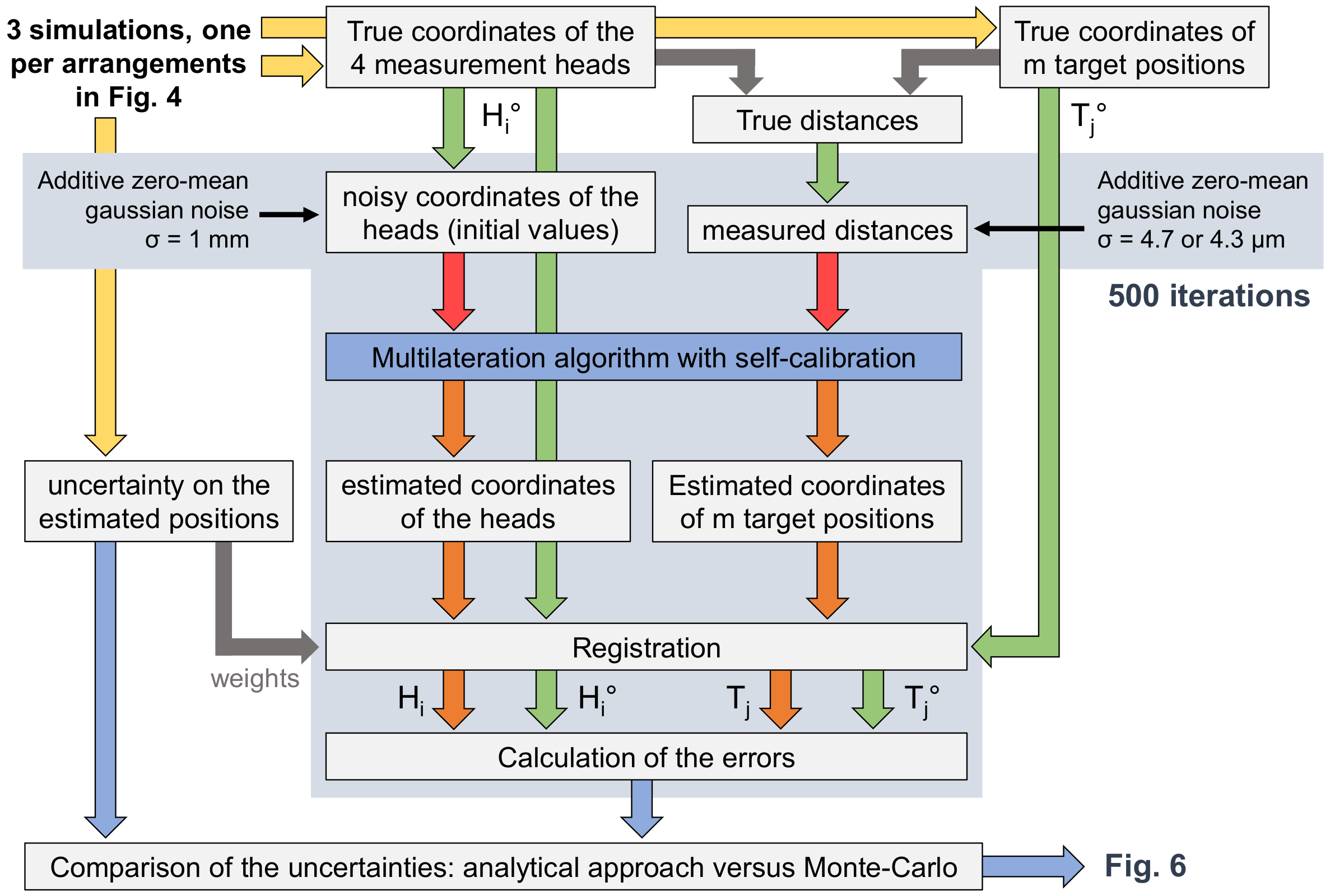
5.2. Monte-Carlo Simulations

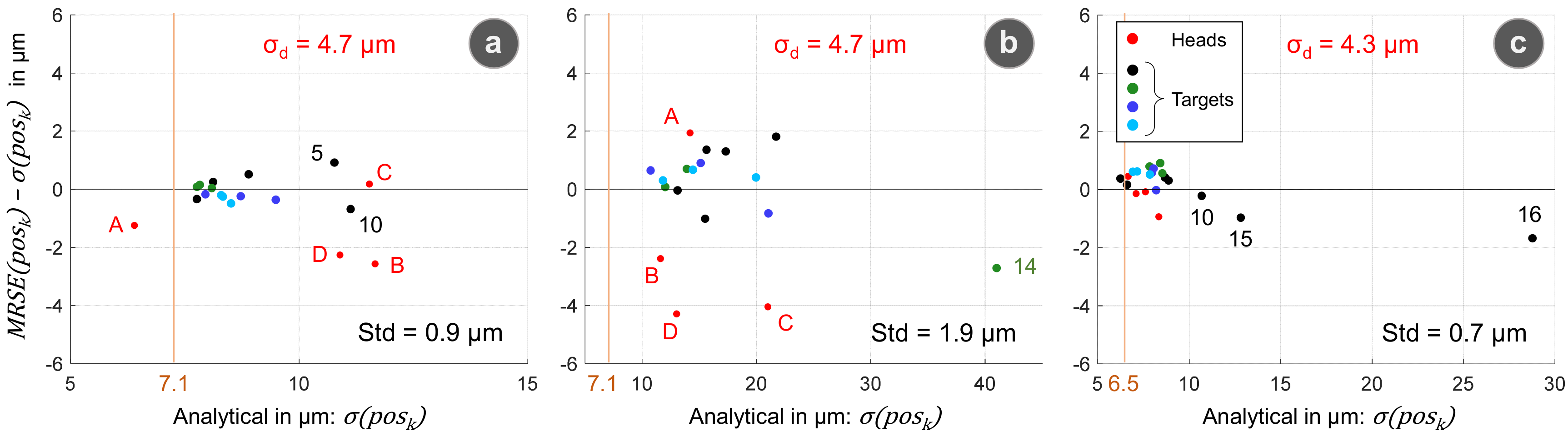
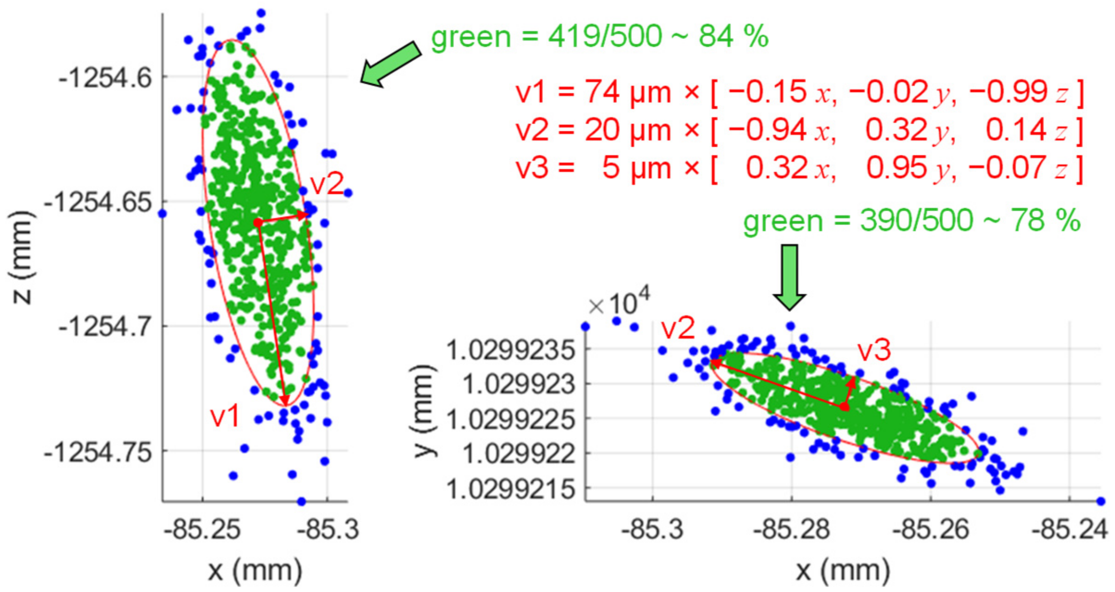
In parallel, Monte-Carlo simulations have been performed. Figure 5 describes how they were constructed.

First, for each geometric arrangement depicted in Figure 4, we calculate the true distances between the measurement heads and the target positions assuming all positions perfectly known. Then, we simulate the measured distances adding a zero-mean Gaussian noise of standard deviation 4.7 µm or 4.3 µm according to the used target, i.e., a corner cube or a glass sphere. We also generate the initial values needed to launch our multilateration algorithm with self-calibration: a zero-mean Gaussian noise of standard deviation 1 mm is thus added to simulate the results of a single head used as a laser tracker. Lastly, the multilateration algorithm is applied and the resulting positions are recorded. It has to be noted that the Monte-Carlo simulations have considered a system that has no instrument offset. The simulated measured distances are therefore not affected by an additional noise due to the instrument offsets. This corresponds to the ideal case described in Section 4.

The Monte-Carlo simulations were made under Matlab^®, and for each simulation, the random sampling of the measured distances and of the initial measurement head coordinates was repeated 500 times. The simulated outputs are positions H_i and T_j, which are compared with the true ones H_i° and T_j°. The true positions are here the results of the experimental measurements. In order to know how well the analytical calculation of the uncertainties fits the Monte-Carlo simulations, a definition of the Monte-Carlo uncertainties has to be provided. It is equal to the mean radial spherical error (MRSE), a single-number indicator used in the global navigation satellite system (GNSS) world [38]:

$$MRSE\left(po{s}_k\right)=\sqrt{\sigma {\left({\mathsf{\Delta }}_x\left(po{s}_k\right)\right)}^2+\sigma {\left({\mathsf{\Delta }}_y\left(po{s}_k\right)\right)}^2+\sigma {\left({\mathsf{\Delta }}_z\left(po{s}_k\right)\right)}^2}$$

(54)

with σ the function that returns the standard deviation and Δ_x, Δ_y and Δ_z the vectors of the differences between the true position k and the positions observed after a Monte-Carlo simulation along each of the three axes. According to [38], the MRSE contains about 61% probability, a confidence region close enough to the one defined in Formula (52) to perform a comparison.

As explained in Section 4.1, the measurement heads are set arbitrarily in a system of coordinates where the head A defines the origin, the head B defines the x axis, and the head C defines the xOy plane. Thus, due to the algorithm design, x_A, y_A, z_A, y_B, z_B, and z_C are always equal to zero and any error cannot be noticed on these coordinates. However, forcing certain coordinates values may result in excessive errors on others. Therefore, before calculating the errors, a registration step based on Horn’s quaternion-based method has been added: this consists of finding a translational vector and a rotational matrix that best match the positions of the heads and targets obtained by multilateration to their true coordinates in a weighted least-squares sense. The applied weights are here the inverse of the square analytical position uncertainties. It has to noted that the uncertainty calculation in Section 4.2 also considered uncertainties for each head so as not to obtain zero uncertainties on some heads and excessive uncertainties on others.

As shown in Figure 5, the MRSE have been compared to the uncertainties calculated analytically from the experimental data, σ(pos_k), as described in Section 4.2.

As previously, a comparison of interpoint distances instead of positions is still relevant. Thus, to complete Table 1, the average value over 500 iterations of some interpoint distances have been reported in the column d₂ as well as the corresponding standard deviation σ₂.

5.3. Results

In Figure 6, the MRSE computed from the Monte-Carlo simulations has been compared to the analytical uncertainties calculated from a set of data randomly generated. The discrepancy between the two approaches is low for the target positions, with errors of few micrometers only. Nevertheless, the results appear less consistent for the measurement heads. In addition, it should be recalled that the analytical uncertainties in Formula (52) represent a confidence region of 68% while MRSE in Formula (54) represents a confidence region around 61%. The MRSE should be lower than the analytical results, which is not necessarily the case.

MRSE and σ(pos_k) are usefull to, respectively, quantify and anticipated the uncertainties of a position using single numbers. However, they do not describe the geometry of the errors. Consequently, the confidence ellipsoids have been directly compared to the results of the Monte-Carlo simulations as shown in Figure 7 with the second configuration, i.e., the large volume, and when the corner cube is located in position 14. This case corresponds to the highest observed uncertainty with a RMSE around 40 µm. In Figure 7, the 500 positions obtained from the Monte-Carlo simulation have been projected on the plane of the confidence ellipse of eigenvectors v1 and v2, then on the plane of the confidence ellipse of eigenvectors v2 and v3. These orthonormal vectors are the eigenvectors of the confidence ellipsoid (at 68%) of the position 14. The red dot corresponds to the true position, while the other dots correspond to the results of the Monte-Carlo simulation, with in green the points inside the ellipse and in blue those outside the ellipse. In theory, the probability that the projections of the three-dimensional points from the simulation on these planes lie within the confidence ellipses is equal to 82.9% [24]. The simulation results are, therefore, very close to the expected values with percentages of 84% for the v1–v2 plane and 78% for the v2–v3 plane. In addition, the shape of the confidence ellipsoid is a good approximation of the shape of the true contour. Figure 6 and Figure 7 validate, therefore, the analytical calculation of the uncertainties.

As shown in Figure 8, the results of the Monte-Carlo simulations were also depicted for the case 3, when a glass sphere is used. For this position, numbered 14, percentages of 80% and 75% were obtained for the v1–v2 and v2–v3 planes, respectively.

At the end, with our system composed of four measurement heads, and for the geometrical arrangements depicted in Figure 4, we typically obtain uncertainties on the positions of both heads and targets between 6 µm and 10 µm for a small volume of one cubic meter and between 10 µm and 22 µm for the large volume. The positions outside the volume formed by the heads have higher uncertainties, for instance the target positions 5 and 10 in case 1, 14 in case 2, 10, 15 and 16 in case 3. However, from the results presented in Section 2.3 for optimal arrangements of the measurement heads, we would expect in Figure 6 uncertainties always higher than 1.5 × σ_d~7 µm (value depicted with an orange vertical line). For instance, in the case 3, the analytical calculation of the uncertainties of the target 14 equals to 6.2 µm, when the corresponding MRSE equals to 6.6 µm. This analytical result is therefore slightly undervalued (by 6%), which is confirmed in Figure 8.

Concerning the interpoint distances, the process to determine their value is recalled in Figure 9 while the results are presented in Table 1. First, the Monte-Carlo simulations, built from data of the experimental measurements, give the same results as the experimental measurements. Then, it has been verified that the experimental results are consistent with the direct distance measurements. Thus, in Figure 10, the distances d₁ and d₃ have been plotted, relatively to the distances d₃ considered here as reference values, with uncertainty bars corresponding to the uncertainties σ₁ and σ₃, respectively. These uncertainty bars are consistent between them for 16 interpoint distances over 24, i.e., 67% of the points lie within one standard deviation (for 68% expected).

As explained previously, in the experimental measurements, four instrument offsets have been determined by the multilateration algorithm with self-calibration in addition to the coordinates of the measurement heads and targets. On the contrary, in the Monte-Carlo simulations, there were no instrument offsets. Nevertheless, in both cases, the uncertainties have been evaluated in the same manner by considering there were no instrument offset.

The consideration of the offsets for the experimental measurements would surely increase the uncertainties of all the positions, and so σ₁. However, in the absence of a mathematical method to determine these uncertainties, the results achieved in Figure 10 show a good agreement between the experimental measurements and the direct measurements.

6. Conclusions

Our objective was to assess with a consistent metrological approach the uncertainties of target positions obtained with our coordinate measurement system. For this purpose, the uncertainty contribution of the data processing has been studied: we have provided an analytical solution for the uncertainty assessment of both targets and heads under different multilateration scenarios.

The original point here was the multilateration algorithm with self-calibration. For this case, we have proposed our own method to assess the uncertainties. First, an approximation of the uncertainties of the coordinates of the heads was calculated from the estimate of Jacobian matrices. The problem was then addressed as a multilateration algorithm with uncertainties on both the distance measurements and the measurement head positions. It was therefore easy to determine the uncertainties of the target positions from the Fisher information matrix (FIM). Lastly, the uncertainties of the coordinates of the heads were refined from the target positions using again the FIM.

This new approach has then been validated, thanks to comparisons between experimental measurements made with our system and Monte-Carlo simulations. It has been demonstrated that the analytical solution for uncertainty assessment provides results very close to the Monte-Carlo simulations, with differences of few micrometres only. Moreover, the confidence ellipsoids provided by the analytical approach describe well the geometry of the errors. It is, therefore, possible to determine the uncertainties in different directions.

At the end, the accuracy that can be achieved with the developed system, when the arrangement of the heads is close to a regular tetrahedron, is typically between 6 µm and 10 µm for a small volume of one cubic meter and between 10 µm and 22 µm for a large volume with distances around 5 m (confidence regions of probability of 68%).

Nevertheless, the proposed solution for the multilateration algorithm with self-calibration has a limitation. The uncertainty assessment of a multilateration measurement with a self-calibration that includes instrument offsets cannot be treated. In such a case, the measured distances are affected by non-zero mean errors, and the proposed mathematical model cannot be used. To address this problem, Monte-Carlo simulations can for instance be performed to generate data sets, and on the basis of these data, predictive uncertainty models can be built, thanks to machine learning.

In the future, new measurement heads will be developed. They will be designed for instrument offsets mechanically stable over time. Thus, the offsets will be determined, thanks to an additional calibration measurement, and then corrected from the measured distances to use a multilateration algorithm with self-calibration that does not need to determine the instrument offsets.

References

1. Guillory, J.; Truong, D.; Wallerand, J.-P. Assessment of the mechanical errors of a prototype of an optical multilateration system. Rev. Sci. Instrum. 2020, 91, 025004. [Google Scholar] [CrossRef] [PubMed] [Green Version]
2. Guillory, J.; Truong, D.; Wallerand, J.-P. Uncertainty assessment of a prototype of multilateration coordinate measurement system. Precis. Eng. 2020, 66, 496–506. [Google Scholar] [CrossRef]
3. Guillory, J.; Truong, D.; Wallerand, J.-P.; Alexandre, C. Absolute multilateration-based coordinate measurement system using retroreflecting glass spheres. Precis. Eng. 2022, 73, 214–227. [Google Scholar] [CrossRef]
4. Zhang, D.; Rolt, S.; Maropoulos, P.G. Modelling and optimization of novel laser multilateration schemes for high-precision applications. Meas. Sci. Technol. 2005, 16, 2541–2547. [Google Scholar] [CrossRef]
5. Bönsch, G.; Potulski, E. Measurement of the refractive index of air and comparison with modified Edlén’s formulae. Metrologia 1998, 35, 133–139. [Google Scholar] [CrossRef]
6. Nitsche, J.; Franke, M.; Haverkamp, N.; Heißelmann, D. Six-degree-of-freedom pose estimation with µm/µrad accuracy based on laser multilateration. J. Sens. Sens. Syst. 2021, 10, 19–24. [Google Scholar] [CrossRef]
7. Rafeld, E.K.; Koppert, N.; Franke, M.; Keller, F.; Heißelmann, D.; Stein, M.; Kniel, K. Recent developments on an interferometric multilateration measurement system for large volume coordinate metrology. Meas. Sci. Technol. 2022, 33, 035004. [Google Scholar] [CrossRef]
8. Nguyen, Q.K.; Kim, S.; Han, S.H.; Ro, S.K.; Kim, S.W.; Kim, Y.J.; Kim, W.; Oh, J.S. Improved Self-Calibration of a Multilateration System Based on Absolute Distance Measurement. Sensors 2020, 20, 7288. [Google Scholar] [CrossRef]
9. Hughes, B.; Campbell, M.A.; Lewis, A.J.; Lazzarini, G.M.; Kay, N. Development of a high-accuracy multi-sensor, multi-target coordinate metrology system using frequency scanning interferometry and multilateration. In Proceedings of the Society of Photo-Optical Instrumentation Engineers (SPIE), Videometrics, Range Imaging, and Applications XIV, Munich, Germany, 26 June 2017; Volume 10332, p. 1033202. [Google Scholar]
10. Salzenstein, P.; Pavlyuchenko, E. Uncertainty Evaluation on a 10.52 GHz (5 dBm) Optoelectronic Oscillator Phase Noise Performance. Micromachines 2021, 12, 474. [Google Scholar] [CrossRef]
11. BIPM Stands for Bureau International des Poids et Mesures, GUM. Guide to the Expression of Uncertainty in Measurement, Fundamental Reference Document, JCGM100: 2008 (GUM 1995 Minor Corrections). Available online: https://www.bipm.org/en/publications/guides (accessed on 28 April 2022).
12. Moona, G.; Kumar, V.; Jewariya, M.; Sharma, R. Measurement uncertainty assessment of articulated arm coordinate measuring machine for length measurement errors using Monte Carlo simulation. Int. J. Adv. Manuf. Technol. 2022, 119, 5903–5916. [Google Scholar] [CrossRef]
13. Tripathy, R.; Bilionis, I.; Gonzalez, M. Gaussian processes with built-in dimensionality reduction: Applications to high-dimensional uncertainty propagation. J. Comput. Phys. 2016, 321, 191–223. [Google Scholar] [CrossRef] [Green Version]
14. Chakraborty, S.; Chowdhury, R. An efficient algorithm for building locally refined hp—adaptive H-PCFE: Application to uncertainty quantification. J. Comput. Phys. 2017, 351, 59–79. [Google Scholar] [CrossRef]
15. D’auria, F.; Debrecin, N.; Galassi, G.M. Outline of the Uncertainty Methodology Based on Accuracy Extrapolation. Nucl. Technol. 1995, 109, 21–38. [Google Scholar] [CrossRef]
16. Navidi, W.; Murphy, W.S., Jr.; Hereman, W. Statistical methods in surveying by trilateration. Comput. Stat. Data Anal. 1998, 27, 209–227. [Google Scholar] [CrossRef]
17. Norrdine, A. An Algebraic Solution to the Multilateration Problem. In Proceedings of the International Conference on Indoor Positioning and Indoor Navigation, Sydney, Australia, 13–15 November 2012. [Google Scholar]
18. Benkouider, Y.K.; Keche, M.; Abed-Meraim, K. Divided Difference Kalman Filter for Indoor Mobile Localization. In Proceedings of the International Conference on Indoor Positioning and Indoor Navigation, Montbeliard-Belfort, France, 28–31 October 2013. [Google Scholar]
19. Yunlong, T.; Shaopu, Y.; Pancunzhi. Research and application of localization algorithm based on wireless sensor networks. In Proceedings of the International Conference on Computer Science and Information Technology (ICCSIT), Chengdu, China, 9–11 July 2010. [Google Scholar]
20. Kay, S.M. Fundamentals of Statistical Signal Processing: Estimation Theory; Prentice Hall: Upper Saddle River, NJ, USA, 1993; p. 141. [Google Scholar]
21. Patwari, N.; Ash, J.N.; Kyperountas, S.; Hero, A.O.; Moses, R.L.; Correal, N.S. Locating the Nodes. IEEE Signal Process. Mag. 2005, 22, 54–69. [Google Scholar] [CrossRef]
22. Chaffee, J.; Abel, J. GDOP and the Cramer-Rao bound. In Proceedings of the Position, Location and Navigation Symposium (PLANS), Las Vegas, NV, USA, 11–15 April 1994; pp. 663–668. [Google Scholar]
23. Mitchell, J.; Spence, A.; Hoang, M.; Free, A. Sensor fusion of laser trackers for use in large-scale precision metrology. In Proceedings of the Photonics Technologies for Robotics, Automation, and Manufacturing, Providence, RI, USA, 27–31 October 2003. [Google Scholar]
24. Wang, B.; Shi, W.; Miao, Z. Confidence analysis of standard deviational ellipse and its extension into higher dimensional euclidean space. PLoS ONE 2015, 10, 17. [Google Scholar] [CrossRef]
25. Lin, Y.; Zhang, G. The optimal arrangement of four laser tracking interferometers in 3D coordinate measuring system based on multi-lateration. In Proceedings of the International Symposium on Virtual Environments, Human-Computer Interfaces and Measurement Systems (VECIMS), Lugano, Switzerland, 27–29 July 2003; pp. 138–143. [Google Scholar]
26. Xue, S.; Yang, Y.; Dang, Y.; Chen, W. A Conditional Equation for Minimizing the GDOP of Multi-GNSS Constellation and Its Boundary Solution with Geostationary Satellites. In IAG 150 Years; International Association of Geodesy Symposia: Postdam, Germany, 2013. [Google Scholar]
27. Ma, Z.; Ho, K.C. TOA localization in the presence of random sensor position errors. In Proceedings of the International Conference on Acoustics, Speech and Signal Processing (ICASSP), Prague, Czech Republic, 22–27 May 2011. [Google Scholar]
28. Kumar, V. Cooperative Localization and Tracking of Resource-Constrained Mobile Nodes. Ph.D. Thesis, School of Information Technology and Electrical Engineering, University of Queensland, Brisbane, QLD, Australia, 2018. Available online: https://espace.library.uq.edu.au/view/UQ:3b1bfbd (accessed on 14 March 2020).
29. Sun, M.; Yang, L.; Ho, K.C. Accurate sequential self-localization of sensor nodes in closed-form. Signal Process. 2012, 92, 2940–2951. [Google Scholar] [CrossRef]
30. Zhuang, H.; Li, B.; Roth, Z.S.; Xie, X. Self-calibration and mirror center offset elimination of a multi-beam laser tracking system. Robot. Auton. Syst. 1992, 9, 255–269. [Google Scholar] [CrossRef]
31. Trébert, A. De la sphère tangente a quatre sphères données. Nouv. Ann. Math. J. Candidats Aux Écoles Polytech. Et Normale. 1844, 3, 101–111. [Google Scholar]
32. Kasmi, Z.; Norrdine, A.; Blankenbach, J. Platform Architecture for Decentralized Positioning Systems. Sensors 2017, 17, 957. [Google Scholar] [CrossRef] [Green Version]
33. Moses, R.L.; Patterson, R. Self-Calibration of Sensor Networks. In Proceedings of the AeroSense, Orlando, FL, USA, 1–5 April 2002. [Google Scholar]
34. Donaldson, J.R.; Schnabel, R.B. Computational experience with confidence regions and confidence intervals for nonlinear least squares. Technometrics 1987, 29, 67–82. [Google Scholar] [CrossRef]
35. D’Errico, J. Adaptive Robust Numerical Differentiation. Numerical Derivative of an Analytically Supplied Function, also Gradient, Jacobian & Hessian, Version 1.6. 2007. Available online: https://fr.mathworks.com/matlabcentral/fileexchange/13490-adaptive-robust-numerical-differentiation (accessed on 14 March 2020).
36. Bell, B. ME5000 Test Measurements. In Proceedings of the Workshop on the Use and Calibration of the Kern ME5000 Mekometer, Standford, CA, USA, 18–19 June 1992. [Google Scholar]
37. Braun, J.; Štroner, M.; Urban, R.; Dvořáček, F. Suppression of Systematic Errors of Electronic Distance Meters for Measurement of Short Distances. Sensors 2015, 15, 19264–19301. [Google Scholar] [CrossRef] [PubMed] [Green Version]
38. Leick, A.; Rapoport, L.; Tatarnikov, D. GPS Satellite Surveying, 4th ed.; John Wiley & Sons: Hoboken, NJ, USA, 2015; p. 61. [Google Scholar] [CrossRef]
Figure 1. Three of the four measurement heads (identified by letters) and the two types of targets.
Metrology 02 00015 g001
Figure 2. Confidence ellipsoid.
Metrology 02 00015 g002
Figure 3. Best arrangements for multilateration with 4 heads: there are three types of geometry (ac) that minimize the uncertainty on the target position.
Metrology 02 00015 g003
Figure 4. Top view of the layouts of the 4 measurement heads and of the targets for the three experimental measurements that were carried out (ac). In the two first cases (a,b), a corner cube is used as target, while in the last case (c), a glass sphere is used as target.
Metrology 02 00015 g004
Figure 5. The Monte-Carlo diagram.
Metrology 02 00015 g005
Figure 6. Comparison between the Monte-Carlo simulations and the analytical calculation of the uncertainties for the three experimental measurements that were carried out (ac). The number of the positions is indicated when the obtained uncertainties are high.
Metrology 02 00015 g006
Figure 7. Case 2—multilateration in a large volume when the target, a corner cube, is in position 14: positions obtained from the Monte-Carlo simulation versus confidence ellipsoid at 68%.
Metrology 02 00015 g007
Figure 8. Case 3—multilateration in a small volume when the target, a sphere, is in position 14: positions obtained from the Monte-Carlo simulation versus confidence ellipsoid at 68%.
Metrology 02 00015 g008
Figure 9. Description of the determination of d1, d2 and d3 and of their associated uncertainties.
Metrology 02 00015 g009
Figure 10. Comparison of the experimental results d1 with the direct distance measurements d3 for the three experimental measurements that were carried out (ac), with uncertainty bars corresponding to confidence intervals of 68% (k = 1).
Metrology 02 00015 g010