Calibration of a Digital Current Transformer Measuring Bridge: Metrological Challenges and Uncertainty Contributions ^†

Abstract

In this paper, we consider the calibration of measuring bridges for non-conventional instrument transformers with digital output. In this context, the main challenge is represented by the necessity of synchronization between analog and digital outputs. To this end, we propose a measurement setup that allows for monitoring and quantifying the main quantities of interest. A possible laboratory implementation is presented and the main sources of uncertainty are discussed. From a metrological point of view, technical specifications and statistical analysis are employed to draw up a rigorous uncertainty budget of the calibration setup. An experimental validation is also provided through the thorough characterization of the measurement accuracy of a commercial device in use at METAS laboratories. The proposed analysis proves how the calibration of measuring bridges for non-conventional instrument transformers requires ad hoc measurement setups and identifies possible space for improvement, particularly in terms of outputs’ synchronization and flexibility of the generation process.

1. Introduction

In view of reducing greenhouse gas emissions and carbon dependence, modern power systems are experiencing an ever-increasing integration of renewable energy sources and distributed generation [1,2]. Such resources are typically connected via dedicated inverters whose power electronics-based control can not guarantee any rotational inertia or regularization of the energy generation profile [3,4]. As a consequence, power systems are expected to face much faster dynamics, as proven by recent adverse events in South Australia and California [5,6].

In order to address such challenges, also the measurement infrastructure needs to undergo a significant renovation, both in terms of instrumentation and control strategies [7]. In particular, the transition from traditional to digital electrical substations paves the way to more sophisticated and optimized approaches for the collection and aggregation of the quantities of interest, e.g., voltage and current levels at the transformer secondary windings [8]. In this context, the recent IEC Std 61869-9:2016 [9] defines the operational and communication requirements for instrument transformer with digital output. Due to their capability of converting the output signal directly in a digital form (and thus compatible with many processing and storage applications), such transformers are typically referred to as non-conventional instrument transformers, briefly NCIT [10].

In terms of communication protocol, the IEC Std 61850-9-2:2011 [11] introduces the Sampled Values (SV): a publisher/subscriber protocol for information exchange between Stand Alone Merging Units (SAMUs) and Intelligent Electronic Devices (IEDs) over the Ethernet. Originally conceived just as an efficient way to concentrate the outputs of NCITs and SAMUs [12,13,14], the SV is now directly applied to more sophisticated processing applications, e.g., phasor measurements [15] and protection schemes [16].

The recent EMPIR project FutureGrid II has been investigating the measurement needs and potential of SVs in modern electrical substations. In particular, dedicated calibration infrastructures for transmitting and receiving SVs have been developed and thoroughly characterized [17,18]. However, a rigorous and well-established procedure for the metrological characterization of NCITs is not yet available. The measurement setup typically includes a transformer measuring bridge capable of processing both analog and digital inputs [19]. The calibration of such device, though, is not straightforward and requires a precise assessment of the several uncertainty sources involved in the measurement process. Indeed, the comparison between purely analog quantities and time-stamped digital values represents a non-negligible challenge, especially in terms of synchronization and phase angle uncertainty.

In this paper, we consider the problem of calibrating a measuring bridge for NCITs from a metrological point of view [20,21]. In particular, we describe a novel measurement setup and discuss the implementation challenges and requirements as well as the possible uncertainty contributions. A preliminary calibration campaign confirms the feasibility and reliability of the proposed approach, and sets a realistic performance target for the uncertainty budget of the calibration infrastructure.

The paper is organized as follows: in Section 2, we present the measurement principle inherent in measuring bridges for traditional and non-conventional transformers. Section 3 outlines the measurement setup for the bridge calibration and describes the actual implementation in METAS laboratories. In Section 4, we discuss the main uncertainty contributions and derive a preliminary uncertainty budget based on technical specifications and statistical analysis. In Section 5, we provide an experimental validation by presenting the results of a measurement campaign on a commercial device. Finally, Section 6 provides some closing remarks and outlines the next steps of the research.

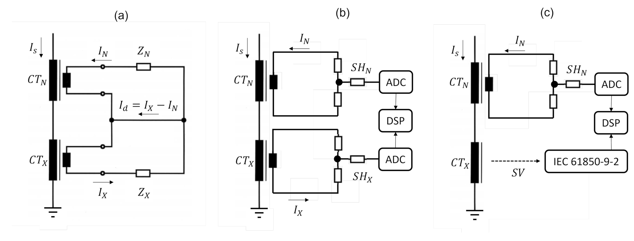
2. Measuring Bridge: Configurations and Measurement Principles

In this section, we briefly describe the measurement principle of measuring bridges for instrument transformers, focusing on the transition from the traditional analog approach to the non-conventional approach based on SV communication protocol. In the following, we refer to the specific case of current transformers but similar considerations apply as well to voltage transformers.

Traditional measuring bridges for instrument transformers rely on the well-known difference method [22]. As shown in Figure 1a, the same current source $I_s$ is supplied to two current transformers: a standard reference transformer, typically referred to as normal (channel N), and the transformer under test (channel X). For the sake of comparability, the two transformers adopt the same transformation ratio. As a consequence, they should produce the same current output at the secondary winding.

It is worth noticing that, in a calibration context, the current source and the normal transformers are subject to periodic and thorough metrological characterization campaigns: systematic errors are suitably compensated, whereas random contribution determine the source stability and the transformer uncertainty, whose levels are guaranteed to be much lower than the expected performance of the device under test.

By means of current sensors (typically, a calibrated shunt and a voltmeter or a digitizer), the measuring bridge determines the current flowing at the secondary winding of the two transformers, $I_N$ and $I_X$, respectively, as well as their difference $I_d=I_X-I_N$. In a vector space rotating at the nominal system frequency (e.g., 50 Hz), it is possible to represent these quantities as rotating vectors, whose magnitude and phase depend on the characteristics of the transformer under test.

Based on these measurements, the measuring bridge calculates the complex transformer or excitation error $\Delta E=I_d/I_N$ (The excitation error is not necessarily included in a calibration report as it depends on the accuracy and stability of the selected current source and reference standard transformer. In this paper, we report also $\Delta E$ as it is one of the measurement values commonly output by a measurement bridge, and thus it might be interesting to associate it with a measurement uncertainty), the transformer ratio error $\Delta \epsilon$, and the phase displacement $\Delta \phi$ (In this paper, the test waveforms consist of sine waveforms. Therefore, a negative phase displacement corresponds to a current $I_X$ that is delayed with respect to the reference current $I_N$).

In Figure 1b, we present an example of new generation of measuring bridges. With the emergence of integrated circuits and fixed-point microprocessors, also measuring bridges have been equipped with Analog-to-Digital Converters (ADCs) and Digital Signal Processing (DSP) units for a more sophisticated treatment of the digitizer outputs. Instead of considering their difference in an analog circuit, each channel is processed independently: by means of a Discrete Fourier Transform (DFT), it is possible to define the complex coefficient associated with the nominal system rate. The comparison between these complex quantities allow for quantifying the excitation and ratio errors and the phase displacements. Moreover, by differentiating the phase information, it is also possible to determine the signal frequency and detect possible distortion introduced in the transformation.

Finally, Figure 1c represents the configuration of a measuring bridge for NCITs. As the transformer under test outputs the current at the secondary winding directly in a digital format, the X channel has to be supplied with an Ethernet board responsible of capturing the SV data packets and aligning them with the samples provided by the ADC on the N channel.

First, the captured SV data packets are queued in a First-In-First-Out (FIFO) buffer. Then, the time-stamp information is extracted and compared with the internal time of the measuring bridge: in the presence of high discrepancies (e.g., delayed transmission), the comparison with the reference channel values is unfeasible and the measuring bridge outputs an error message due to synchronization loss. Otherwise, the analog quantities are extracted from the SV data packets and transmitted to the DSP for the DFT processing and the error computation.

In this regard, it is reasonable to assume that the excitation error $\Delta E$ is mostly dependent on the accuracy and stability of the current measurement at the N-channel. In the absence of synchronization or packet loss, the SV data stream is characterized by a constant amplitude whose accuracy depends only on the quantization error and on possible numerical errors in the bridge DSP. On the contrary, $I_N$ is an analog quantity that might vary as function of time, depending on the stability of the current source and on the characteristic of the standard transformer $C{T}_N$.

3. Measurement Setup

In this section, we present the measurement setup for the metrological characterization of a measuring bridge for non-conventional instrument transformers. Indeed, a detailed analysis of the employed instruments and measurement techniques is crucial in view of the uncertainty analysis in the following section.

As shown in Figure 2, the setup consists of six main components: a time reference, a calibrator, a transconductance amplifier, a calibrated shunt, a set of synchronized voltmeters, and the Device Under Test (DUT), i.e., the measuring bridge.

The time reference is responsible for providing the calibrator with a refined and stable time-base. To this end, a 10-MHz signal overrides the internal clock of the calibrator. It is worth noticing that, in such application, the traceability to Universal Time Coordinate (UTC) time is not mandatory. The only constraint is the exact synchronization between the calibrator analog and digital outputs, as well as between the calibrator and the measuring bridge.

The calibrator consists of three main units:

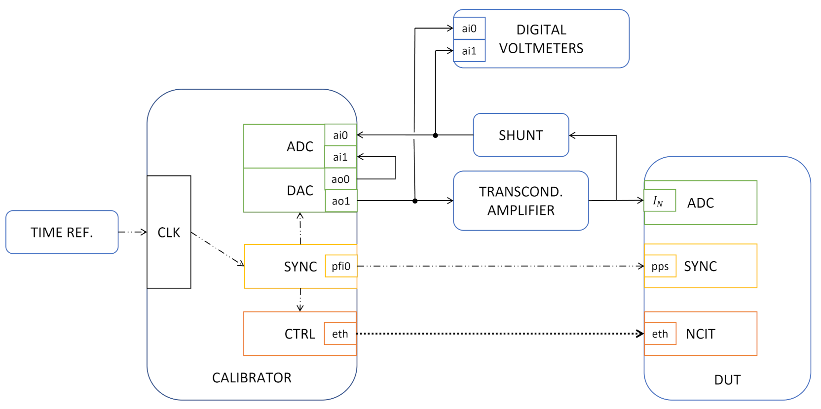
• A digital acquisition unit with a Digital-to-Analog Converter (DAC) and an ADC that operate in simultaneous mode, i.e., share the same time-base and sampling rate. The DAC is responsible for generating the analog test waveform to be supplied at the transconductance amplifier and then the DUT, whereas the ADC simultaneously re-acquires the same waveform to make it available for further processing and defining the actual reference values. In this context, it should be noticed that both DAC and ADC are typically equipped with two channels. One pair of channels (ai0 and ao1 in Figure 2) is dedicated to the test waveform generation and re-acquisition, whereas the other one (ai1 and ao0) is intended for self-calibration tasks, namely for the definition of the DAC phase offset [18], as further discussed in the following section;
• A synchronization unit locked to the internal clock, and thus to the external time reference. The synchronization board is responsible for two main tasks: distributing the triggers for the other units within the calibrator, and providing the measuring bridge with a Pulse-Per-Second (PPS) signal that is aligned with the time-stamp of the SV data packets. As regards the first task, the main difficulty is represented by the necessity of simultaneously triggering a purely hardware unit, namely the DAQ, and a purely software process, namely the SV transmission. To this end, software defined triggers are programmed as future time events, i.e., in correspondence of the first rising edge of the internal time base after a given time instant. As regards the second task, instead, the PPS is generated as a Transistor-Transistor Logic (TTL) signal, disciplined at the same rising edge as the software triggers;
• A controller unit with sufficient memory and processing capabilities, and an Ethernet board. On one side, the controller supervises the DAQ unit: it defines the test waveform to be generated as a sample series at the given sampling rate, stores the acquired samples, and processes them in order to estimate (in quasi real-time) the DAC phase offset. On the other side, the controller is responsible for publishing the SV data packets, from the encapsulation of the SV to the actual transmission through a dedicated Ethernet board.

The DAC outputs a low-voltage sinusoidal signal, in the range of ±2 V. The amplitude, frequency and initial phase of the signal can be customized to specific test conditions. The conversion to the current levels expected by the N channel of the measuring bridge is carried out by a transconductance amplifier. In this sense, the amplifier ratio represents a further degree of freedom in view of a finer control of the current level, and thus of the excitation. The transconductance amplifier is not an ideal current source and introduces non-negligible uncertainty contributions on both the amplitude and phase of the signal supplied to the measuring bridge.

The ADC re-acquires the amplifier output by means of a calibrated high-precision shunt whose input range is suitably adapted to the specific test configuration. Typically, the shunt output is scaled such that a full input range corresponds to an output range of 0.8 V. Given the calibration context and the high-accuracy of the employed shunts, their contribution in terms of amplitude and phase uncertainty can be reasonably considered as negligible, as further discussed in the next section.

The time-series acquired at the two ADC input channels are processed via a DFT-based routine (further details in [18]) and the phase associated with the fundamental frequency is retrieved. In particular, channel ai1 is representative of the contribution of ADC only, whereas channel ai0 is representative of the entire measurement chain. By properly differentiating these terms, it is possible to define the actual phase of the signal supplied to the measuring bridge.

In the top-centre part of the scheme, a pair of Digital Voltmeters (DVMs) monitors the input and output signal of the series of transconductance amplifier and shunt. The DVMs are employed as high-precision sampling systems that operate in simultaneous mode: the acquired time series are processed via a sine fitting method that allows for accurately estimating the amplitude, frequency and initial phase of the signals under analysis. The DVMs’ trigger is not synchronous with the PPS of the synchronization unit, neither is it disciplined to the time reference. As a consequence, the phase information cannot be related to the phase measured on the calibrator. Nevertheless, the difference between the phase measured on each DVM allows for quantifying the phase offset introduced by the amplifier only. It is therefore an independent method to validate the results of DFT-based routine carried out on the re-acquired waveforms.

METAS Implementation

As implemented in the METAS laboratories, the different components of the measurement setup are listed here below.

• Time reference: A Meinberg LANTIME M600Time Server (Meinberg Funkuhren, Bad Pyrmont, Germany) that includes a GPS-disciplined 10-MHz clock, whose time accuracy and frequency stability are in the order of 50 ns and 0.5 nHz/Hz over an averaging time of 1800 s, respectively [17].
• Calibrator: An NI PXIe 1062 chassis (National Instruments, Austin, TX, USA) that hosts three boards: the NI PXIe 8880 controller, the NI PXI 6683 timing and synchronization module, and the NI PXI 4461 dynamic signal acquisition module. The NI PXIe 8880 is an Intel Xeon embedded controller (2.3 GHz Eight-Core) with two 10/100/1000BASE-TX (Gigabit) Ethernet ports. The NI PXI 6683 can generate events and clock signals at specified synchronized future times and timestamp input events with the synchronized system time. The NI PXI 4461 is a 2-input/2-output DAQ with a nominal resolution of 24 bits. The sampling rate and the vertical range are set equal to 192 kHz and ±2 V, respectively, for both DAC and ADC channels.
• Transconductance amplifier: A Clarke-Hess 8100 (Clarke-Hess, Medford, NY, USA) characterized by a 50 ppm short-term stability, a maximum compliance voltage of 7 V, a total harmonic distortion lower than −60 dB up to 10 kHz, and six available output range from 200 mA to 100 A.
• Shunt: A set of Fluke A40B Precision DC and AC Current Shunts (Fluke, Norwich, UK) with a worst-case uncertainty of 55 ppm up to 1 kHz signal frequency. In particular, we adapted the shunt input range to the generated current level: a 500-mA shunt for $50\le I_N<500$ mA, and a 10-A shunt for $1\le I_N\le 10$ A. In this sense, a further improvement might be represented by the adoption of magnetoresistance sensors. Nevertheless, it should be noticed that the shunts are periodically calibrated and thus the non-ideal conversion ratio is suitably compensated, and its effect is negligible if compared to the calibrator and amplifier ones.
• Digital Voltmeters: A pair of Keysight 3458A Multimeters (Keysight Technologies, Santa Rosa, CA, USA) with a resolution of 8.5 digits and an accuracy of 100 ppm in synchronous mode. The DVMs are used as digitizers for a sine fitting technique with a sampling rate of 2.5 kHz and an aperture time of 920 $\mathsf{\mu }$s. The two digitizers operate in a master–slave configuration: the one connected to the calibrator output triggers also the acquisition of the one connected to the amplifier output. In this way, they mimic a two-channel ADC operating in synchronous sampling mode, as further discussed in [23]. It is also worth noticing that the sine fitting procedure returns the value of the amplitude, frequency and initial phase of the fundamental component. Therefore, by comparing the phase at the two channels, we can retrieve the phase contribution of the amplifier only with a standard uncertainty of 0.03 $\mathsf{\mu }$rad [24].
• Measuring bridge (DUT): A ZERA WM3000I (ZERA, Konigswinter, Germany) with a current input range from 1 mA to 15 A. In non-conventional mode, the bridge guarantees a ratio and phase uncertainty not larger than 300 ppm and 1.5 min, respectively.

4. Uncertainty Contributions

In this section, we analyse the main uncertainty sources inherent in the proposed measurement setup and we derive a complete uncertainty budget based on technical specifications and statistical analysis (In case of statistical analysis, a coverage factor $k=2$ (i.e., 95%) has been applied to the standard deviations).

In this context, four main contributions can be identified. Three descend from the measurement chain for the generation and re-acquisition of the analog test waveform, i.e., from the DAQ module, the transconductance amplifier and (marginally) the current shunt. One contribution, instead, is directly related to the definition of the SV data packets, i.e., to the vertical resolution loss due to quantization effects.

As regards the DAQ module, two synchronization aspects have to be taken into account: the sampling rate and the phase offset introduced by an improper triggering of the DAC and ADC boards. The sampling rate is derived from the internal time base that is disciplined to the external time reference. In our setup, we are able to retrieve the coerced sampling rate on both boards and the discrepancy between nominal and actual sampling rate is equal to 0.3 ppb [18]. Therefore, it is reasonable to say that the sampling rate has a negligible effect on the amplitude, frequency and phase of the generated and re-acquired waveform.

By connecting the channels ao1 and ai0, we were able to quantify also the distortion level introduced by the DAQ module. In the considered configuration, we evaluated a worst-case Signal-to-Noise Ratio (SNR) and a Total Harmonic Distortion of 92 and −96 dB, respectively. As a consequence, the effective number of bits is equal to 17 bits. In this respect, it should be noticed that such levels of accuracy require a precise control of temperature and power supply stability. In our case, the measurement campaign has been carried out in METAS laboratories with a controlled temperature of 23 Celsius degrees and adopting a power supply at 60 Hz for all the instrumentation, i.e., calibrator, amplifier and DUT, to avoid beating effects or interferences. For this analysis, we considered a dataset of 100 independent acquisition with a sample length of 4 s. Moreover, we quantified the purity of the test waveform by means of a nonlinear fit against a single-tone sinusoidal model that produced a Goodness-of-Fit index not lower than 99.7% [18]. Based on these considerations, we quantified the DAQ contribution to the estimation of the current amplitude in terms of the noise variation range. By also taking into account the integral nonlinearity of the ADC board, as characterized in [25], for a test waveform amplitude of 1 V, the uncertainty is 25.12 ppm.

A further validation of this result is provided by the RMS measurements carried out by the first channel of the DVM system. For this analysis, we considered a dataset of 200 measurements and evaluated the mean and standard deviation. As shown in Figure 3, the distribution is well approximated by a Gaussian distribution and the uncertainty can be quantified in the worst-case in 23.71 ppm. The peculiar non-monotonic uncertainty trend depends also on the adoption of two current shunts with different input range (namely, 500 mA and 10 A), as previously introduced.

The second synchronization aspect regards the triggering mechanism of DAC and ADC boards, with respect to the PPS signal output by the synchronization board (and the time-stamp of the digital data stream). In this regard, it should be noticed that the DAQ module relies on a Sigma-Delta technology: the phase offset introduced by the analog front end of DAC and ADC boards is dependent on the sampling rate. Nevertheless, in a calibration context, it is possible to characterize such contribution and minimize its systematic component by properly shifting the initial phase of the generated waveform. To this end, it is necessary to quantify precisely the phase offset introduced by DAC and ADC boards separately. In recent years, this problem has been widely investigated by several metrological institutes [26,27,28]. In our measurement setup, we adopted a DFT-based routine for the precise characterization of the phase offset of the signal supplied to the transconductance amplifier. The algorithmic details are beyond the scope of this analysis but can be found in [18]. At 50 Hz, the phase offset has been proven to exhibit a normal distribution with mean and standard deviation equal to 4.186 mrad and 0.004 mrad, respectively. The first one can be seen as a systematic contribution and thus compensated, whereas the second one is a random variable and is related to the phase uncertainty introduced by the DAQ module.

In this context, another aspect that should not be neglected is the proper alignment of the software triggers with the PPS used to synchronize the measuring bridge. With respect to the external time-reference, we quantified the delay introduced by the calibrator in the software triggers and in the PPS output of the synchronization module. As regards the first ones, the technical specifications guarantee the rising edge to occur within 5 ns of the selected time-stamp. Moreover, it should be noticed that the synchronization module guarantees the distribution of software triggers to neighbouring modules (as the DAQ and the controller) with a maximum delay of 2 ns. As regards the PPS output, we employed a high-precision digital oscilloscope with a sampling rate of 2 GHz and we compared the PPS output against the external time reference. Over an observation interval of nearly 10 min, the PPS showed an average delay of 10 ns with a jitter on the order of few ps. These contributions sum up to 11.36 ns that corresponds to a phase uncertainty of 3.568 $\mathsf{\mu }$rad.

Once output by the calibrator, the transconductance amplifier converts the voltage test waveform in the corresponding current waveform. In order to characterize the amplitude and phase contributions of this stage, this signal is re-acquired through a high-accuracy current shunt. It is worth noticing that the shunts (periodically calibrated) contribute to the overall uncertainty by at most 0.90 ppm for the amplitude, and 1.50 $\mathsf{\mu }$rad for the phase [29,30]. On the other hand, the transconductance amplifier has a much more significant impact on the overall uncertainty. As per the calibrator output, we analysed the amplifier output via the DVM. In this case, we were also able to compute the phase displacement between the two channels, i.e., the phase displacement introduced by the transconductance amplifier (and the shunt). For each considered current level, we carried out 200 independent measurements and computed the corresponding statistical distributions: the mean value is taken as a systematic contribution and thus compensated, the standard deviation is used for the uncertainty computation. Figure 4 presents the uncertainty associated with amplitude and phase as function of the current level. In the worst-case, the former is equal to 160.75 ppm, whereas the latter is 200 $\mathsf{\mu }$rad. In this regard, it is worth noticing how the uncertainty rapidly increases when the current levels fall below 500 mA. Indeed, the selected amplifier is designed for high current output and exhibits a poor accuracy at lower current levels. At the nominal value of 5 A, the uncertainty for amplitude and phase are just 8.36 ppm and 8 $\mathsf{\mu }$rad, respectively.

Finally, the contribution of the digital output has been also assessed. The SV communication protocol provides a resolution of 32 bits for the analog converted quantities. In terms of quantization error, this corresponds to an amplitude uncertainty of 67 ppm. In terms of phase uncertainty, it is reasonable to set it equal to zero, as the calibrator outputs simulated packets, and thus no conversion error is possible (differently from the digital stream output by a NCIT or a SAMU where measurement errors might occur). On the other hand, it is difficult to merge such uncertainty contributions with the ones related to the analog measurement chain without knowing the algorithm employed by the measuring bridge for the definition of amplitude and phase on the X-channel. If a DFT-based approach is adopted (as in many other SV-based estimators), the recent literature has proven how the amplitude and phase uncertainty due to quantization errors decreases significantly as the resolution of the quantized samples exceed 14 bits [31]. Therefore, for the purpose of this paper, this contribution can be reasonably considered negligible.

As a summary, in

Table 1. Uncertainty budget for amplitude and phase accuracy (coverage factor $k=2$).

	Amplitude Uncertainty	Phase Uncertainty
	${\mathit{U}}_{{\mathit{I}}_{\mathit{N}}}$ (ppm)	${\mathit{U}}_{\mathit{\phi }}$(${}^{\prime }$)
Synchronization module	−	0.012
DAQ module	25.12	0.007
Transconductance amplifier	160.75	0.687
Combined Uncertainty	162.70	0.687

, we report the overall uncertainty budget for the calibration infrastructure. By applying a conservative approach, the combined uncertainty has been computed under the assumption of independent and uncorrelated contributions. Consistently with the common practice in current transformer calibration, the phase uncertainty has been expressed in minutes. In total, the amplitude and phase uncertainty are lower than 200 ppm and 0.7${}^{\prime }$ for the entire range of considered test conditions.

5. Experimental Validation

In this section, we present the results of an experimental validation carried out on the selected DUT, i.e., the ZERA WM3000I. This is intended as an experimental validation of the proposed calibration method as well as of its main uncertainty contributions in controlled laboratory testing conditions, as typical of metrological institute activities. In the following tables, the reported uncertainty takes into account both the calibration setup contribution and the statistical dispersion of the measurements of the device under test. For the sake of readability, a ceiling to the last significant digit has been applied.

For this analysis, we set the nominal frequency, current range and transformer ratio equal to 50 Hz, 5 A and 1:1. Otherwise differently stated, the signals at N- and X-channel consist of single-tone sinusoids, whose frequency, amplitude and initial phase are set equal to 50 Hz, 5 A, and 0 rad, respectively. In the following tests, such parameter values are suitably modified in order to reproduce different configurations of excitation, ratio and phase error, and thus span the entire operating range of the measuring bridge.

To this end, a total of 27 different configurations are taken into account. Each test has a duration of 5 min, including 1 min of settling time to allow for the proper stabilization of the current output of the transconductance amplifier. For each of the monitored quantities, 11 consecutive measurements are taken and their average and standard deviation values are employed to determine the corresponding measurement errors and uncertainties (In the presence of outliers, single measurements could be neglected. In this sense, the outlier detection criterion is based on the assumption that the measurements are normally distributed. Given a set of 11 measurements, if a single measurements differs from the average value by more than three standard deviations, its value is discarded from the computation of measurement errors and uncertainties). In more detail, the reported uncertainties for the excitation and ratio error, and for the phase displacement are obtained by merging the contributions of the calibration setup with the Type A uncertainty of the measuring bridge results.

For the sake of comparison,

Table 2. Specifications of the measuring bridge under test.

Measurement	Accuracy	Current Range
$I_N$, Normal current RMS	100 ppm	$0.05<I_s\le 15$ A
	200 ppm	$0.05\le I_s<0.005$ A
$\Delta \epsilon$, Ratio error	100 ppm	$0.05<I_s\le 15$ A
	200 ppm	$0.05\le I_s<0.005$ A
$\Delta \phi$, Phase displacement	1.1${}^{\prime }$	$0.05<I_s\le 15$ A
	1.5${}^{\prime }$	$0.05\le I_s<0.005$ A

reports the WM3000I specifications in terms of accuracy for the current measurement on the N-channel, the ratio error and the phase displacement. As previously observed, the excitation error in non-conventional mode descends directly from the accuracy of the measured $I_N$ amplitude, as the $I_X$ amplitude depends only on quantization and numerical errors whose impact on the overall uncertainty can be considered as negligible.

In this context,

Table 3. Characterization of the measuring bridge performance in the presence of ratio errors and phase displacements (coverage factor $k=2$).

Settings					Measurements			Uncertainty
${\mathit{I}}_{\mathit{N}}$	${\mathit{I}}_{\mathit{X}}$	$\mathit{E}$	$\epsilon$	$\phi$	$\Delta \mathit{E}$	$\Delta \epsilon$	$\Delta \phi$	${\mathit{U}}_{\Delta \mathit{E}}$	${\mathit{U}}_{\Delta \epsilon }$	${\mathit{U}}_{\Delta \phi }$
(A)	(A)	(%)	(%)	(${}^{\prime }$)	(%)	(%)	(${}^{\prime }$)	(%)	(%)	(${}^{\prime }$)
5	5	100	−5.000	0.00	0.00	−0.003	−0.9	0.02	0.012	1.0
5	5	100	−3.000	0.00	0.00	−0.004	−0.9	0.02	0.012	1.0
5	5	100	−0.200	0.00	0.00	−0.004	−0.9	0.02	0.012	1.0
5	5	100	−0.200	−10.00	0.01	−0.006	−0.9	0.02	0.012	1.0
5	5	100	−0.200	10.00	0.01	−0.006	−0.9	0.02	0.012	1.0
5	5	100	0.000	−5400.00	0.01	−0.005	−0.9	0.02	0.012	1.0
5	5	100	0.000	−180.00	0.01	−0.004	−0.9	0.02	0.012	1.0
5	5	100	0.000	−1.00	0.01	−0.005	−0.9	0.02	0.012	1.0
5	5	100	0.000	0.00	0.01	−0.005	−0.9	0.02	0.012	1.0
5	5	100	0.000	1.00	0.01	−0.006	−0.9	0.02	0.012	1.0
5	5	100	0.000	180.00	0.01	−0.005	−0.9	0.02	0.012	1.0
5	5	100	0.000	5400.00	0.01	−0.005	−0.9	0.02	0.012	1.0
5	5	100	0.000	10,794.00	0.01	−0.005	−0.9	0.02	0.012	1.0
5	5	100	0.200	0.00	0.01	−0.005	−0.9	0.02	0.012	1.0
5	5	100	0.200	−10.00	0.01	−0.005	−0.9	0.02	0.012	1.0
5	5	100	0.200	10.00	0.01	−0.006	−0.9	0.02	0.012	1.0
5	5	100	3.000	0.00	0.01	−0.004	−0.9	0.02	0.012	1.0
5	5	100	5.000	0.00	0.01	−0.005	−0.8	0.02	0.012	1.0

reports the measurement results in the presence of ratio and phase errors. For this analysis, the ratio error is varied within $\pm 5\%$ and the phase displacement is set in such a way to consider small offsets (e.g., $\pm {10}^{\prime }$), large offsets (e.g., $\pm {5400}^{\prime }$), and nearly phase opposition conditions (e.g., $10,{794}^{\prime }$) (Such variations have been obtained by modifying the content of the SV data packets, as the digital channel is characterized by lower uncertainty contributions. Nevertheless, similar results could be obtained by keeping unaltered the SV data packets and suitably modifying the current source flowing through the standard transformer).

The two phenomena are investigated both independently and simultaneously. In this way, it is possible to evaluate whether the measuring bridge is affected by any of the error source or by their combination.

As the excitation is kept equal to 100%, it is worth noticing as the measuring bridge exhibits an excitation error perfectly in line with its specifications and the uncertainty does not exceed 200 ppm. Similar considerations apply for ratio error and phase displacement. In this case, it is interesting to notice how $\Delta \epsilon$ and $\Delta \phi$ do not exhibit any dependence on the test setting.

In

Table 4. Characterization of the measuring bridge performance in the presence of different excitation levels (coverage factor $k=2$).

Settings					Measurements			Uncertainty
${\mathit{I}}_{\mathit{N}}$	${\mathit{I}}_{\mathit{X}}$	$\mathit{E}$	$\epsilon$	$\phi$	$\Delta \mathit{E}$	$\Delta \epsilon$	$\Delta \phi$	${\mathit{U}}_{\Delta \mathit{E}}$	${\mathit{U}}_{\Delta \epsilon }$	${\mathit{U}}_{\Delta \phi }$
(A)	(A)	(%)	(%)	(${}^{\prime }$)	(%)	(%)	(${}^{\prime }$)	(%)	(%)	(${}^{\prime }$)
5	5	1	0.000	0.00	0.00	−0.017	−1.1	0.02	0.028	2.0
5	5	2	0.000	0.00	0.00	0.013	−1.0	0.02	0.017	1.5
5	5	5	0.000	0.00	0.00	−0.009	−1.0	0.02	0.013	1.0
5	5	10	0.000	0.00	0.00	−0.007	−1.1	0.02	0.012	1.0
5	5	20	0.000	0.00	0.00	−0.009	−1.0	0.02	0.012	1.0
5	5	50	0.000	0.00	0.00	−0.006	−0.9	0.02	0.012	1.0
5	5	100	0.000	0.00	0.01	−0.004	−0.9	0.02	0.012	1.0
5	5	120	0.000	0.00	0.01	−0.004	−0.9	0.02	0.012	1.0
5	5	200	0.000	0.00	0.01	−0.001	−1.0	0.02	0.012	1.0

, we report the measuring bridge errors and uncertainties in the presence of different excitation levels. For this analysis, we modified the N-channel current in such a way that the measuring bridge senses an excitation between 1 and 200%. Once more, the excitation error and the corresponding uncertainty are in line with the previous considerations. As regards ratio error and phase displacement, it is worth noticing how both measurements and uncertainties present a rapid increase as the excitation falls below 5%. Nevertheless, it is reasonable to expect that, in the presence of lower current levels, the accuracy of the internal sensors as well as the SNR decrease and the corresponding computations are affected by larger errors and uncertainties. Similar considerations hold also for the digital counterpart. The SV data format has a fixed range and number of bits: as a consequence, when transmitting low-amplitude signals, there is an inefficient exploitation of the 32 bits and the resulting estimates are likely to be affected by higher relative uncertainty.

The specific device under test provides a useful extra feature, i.e., a representation of the current flowing in the N-and X-channel as rotating vectors characterized in terms of RMS amplitude, phase, and frequency. The estimation accuracy of the first two parameters has been already investigated in the previous tables, but the frequency (particularly, the one of the N-channel) requires a separate investigation. To this end, we characterized the frequency measurements in the presence of different excitation levels and phase displacements. For the sake of consistency, the variation ranges of E and $\phi$ correspond to the ones applied in Table 3 and Table 4.

In this context,

Table 5. Characterization of the measuring bridge frequency estimation accuracy in the presence of different excitation levels and phase displacements (coverage factor $k=2$).

Settings						Measurements	Uncertainty
${\mathit{I}}_{\mathit{N}}$	${\mathit{I}}_{\mathit{X}}$	$\mathit{E}$	$\epsilon$	$\phi$	$\mathit{f}$	$\Delta \mathit{f}$	${\mathit{U}}_{\Delta \mathit{f}}$
(A)	(A)	(%)	(%)	(${}^{\prime }$)	(Hz)	(mHz)	(mHz)
5	5	1	0.000	0.00	50	−0.511	0.056
5	5	2	0.000	0.00	50	−0.512	0.038
5	5	5	0.000	0.00	50	−0.556	0.028
5	5	10	0.000	0.00	50	−0.519	0.030
5	5	20	0.000	0.00	50	−0.537	0.031
5	5	50	0.000	0.00	50	−0.537	0.032
5	5	100	0.000	0.00	50	−0.509	0.028
5	5	100	0.000	−5400.00	50	−0.529	0.032
5	5	100	0.000	−180.00	50	−0.557	0.028
5	5	100	0.000	−1.00	50	−0.521	0.030
5	5	100	0.000	0.00	50	−0.530	0.032
5	5	100	0.000	1.00	50	−0.530	0.032
5	5	100	0.000	180.00	50	−0.548	0.030
5	5	100	0.000	5400.00	50	−0.548	0.032
5	5	100	0.000	10,794.00	50	−0.548	0.030
5	5	120	0.000	0.00	50	−0.528	0.032
5	5	200	0.000	0.00	50	−0.511	0.028

reports the measurement results and the associated uncertainty. It is worth noticing how the frequency error $\Delta f$ is quite stable around −0.54 mHz with a worst-case uncertainty of 0.06 mHz (when the excitation is set to its minimum value, i.e., 1%). In this case, the instrument specifications do not provide a performance target. Nevertheless, the obtained measurement accuracy is sufficient for the typical application of a measuring bridge for instrument transformers.

6. Conclusions

In this paper, we presented the measurement setup for the calibration of measurement bridges for non-conventional instrument transformers. We have discussed the main implementation challenges and characterized the most significant uncertainty contributions. Based on technical specifications and statistical analysis, we have performed a comprehensive uncertainty budget of the calibration setup that has been further validated by an experimental measurement campaign carried out at METAS laboratories.

The proposed analysis allows for identifying the main challenges of a calibration process that requires a synchronous generation of both analog and digital quantities. The research project will now focus on the minimization of the uncertainty contributions (with specific attention to the analog measurement chain) and on the extension of the proposed infrastructure to non-stationary signals, as the ones that a plausible instrument transformer might deal with in field applications.

References

1. Terzija, V.; Valverde, G.; Cai, D.; Regulski, P.; Madani, V.; Fitch, J.; Skok, S.; Begovic, M.M.; Phadke, A. Wide-Area Monitoring, Protection, and Control of Future Electric Power Networks. Proc. IEEE 2011, 99, 80–93. [Google Scholar] [CrossRef]
2. Blaabjerg, F.; Yang, Y.; Yang, D.; Wang, X. Distributed Power-Generation Systems and Protection. Proc. IEEE 2017, 105, 1311–1331. [Google Scholar] [CrossRef] [Green Version]
3. Paolone, M.; Gaunt, T.; Guillaud, X.; Liserre, M.; Meliopoulos, S.; Monti, A.; Van Cutsem, T.; Vittal, V.; Vournas, C. Fundamentals of power systems modelling in the presence of converter-interfaced generation. Electr. Power Syst. Res. 2020, 189, 106811. [Google Scholar] [CrossRef]
4. Frigo, G.; Pegoraro, P.; Toscani, S. Low-Latency, Three-Phase PMU Algorithms: Review and Performance Comparison. Appl. Sci. 2021, 11, 2261. [Google Scholar] [CrossRef]
5. Frigo, G.; Derviškadić, A.; Zuo, Y.; Paolone, M. PMU-Based ROCOF Measurements: Uncertainty Limits and Metrological Significance in Power System Applications. IEEE Trans. Instrum. Meas. 2019, 68, 3810–3822. [Google Scholar] [CrossRef] [Green Version]
6. Karpilow, A.C.; Derviskadic, A.; Frigo, G.; Paolone, M. Characterization of Non-Stationary Signals in Electric Grids: A Functional Dictionary Approach. IEEE Trans. Power Syst. 2021, 37, 1–13. [Google Scholar] [CrossRef]
7. Rietveld, G.; Wright, P.S.; Roscoe, A.J. Reliable Rate-of-Change-of-Frequency Measurements: Use Cases and Test Conditions. IEEE Trans. Instrum. Meas. 2020, 69, 6657–6666. [Google Scholar] [CrossRef]
8. Ingram, D.M.E.; Schaub, P.; Campbell, D.A. Use of Precision Time Protocol to Synchronize Sampled-Value Process Buses. IEEE Trans. Instrum. Meas. 2012, 61, 1173–1180. [Google Scholar] [CrossRef] [Green Version]
9. IEEE/IEC International Standard-Instrument transformers-Part 9: Digital interface for instrument transformers. In IEC/IEEE 61869-9:2016; IEC: Geneva, Switzerlad, 2016; pp. 1–127. [CrossRef]
10. Mohns, E.; Mortara, A.; Cayci, H.; Houtzager, E.; Fricke, S.; Agustoni, M.; Ayhan, B. Calibration of Commercial Test Sets for Non-Conventional Instrument Transformers. In Proceedings of the 2017 IEEE International Workshop on Applied Measurements for Power Systems (AMPS), Liverpool, UK, 20–22 September 2017; pp. 1–6. [Google Scholar] [CrossRef]
11. IEC/IEEE International Standard-Communication networks and systems for power utility automation—Part 9-2: Specific Communication Service Mapping (SCSM) Sampledvalues over ISO/IEC 8802-3. In IEC 61850-9-2:2011+AMD1:2020 CSV Consolidated Version 2020-02; IEC: Geneva, Switzerlad, 2011; pp. 1–18. [CrossRef]
12. Castello, P.; Ferrari, P.; Flammini, A.; Muscas, C.; Rinaldi, S. An IEC 61850-Compliant distributed PMU for electrical substations. In Proceedings of the 2012 IEEE International Workshop on Applied Measurements for Power Systems (AMPS) Proceedings, Aachen, Germany, 26–28 September 2012; pp. 1–6. [Google Scholar] [CrossRef]
13. Giustina, D.D.; Dedè, A.; Invernizzi, G.; Valle, D.P.; Franzoni, F.; Pegoiani, A.; Cremaschini, L. Smart Grid Automation Based on IEC 61850: An Experimental Characterization. IEEE Trans. Instrum. Meas. 2015, 64, 2055–2063. [Google Scholar] [CrossRef]
14. Blair, S.M.; Roscoe, A.J.; Irvine, J. Real-time compression of IEC 61869-9 sampled value data. In Proceedings of the 2016 IEEE International Workshop on Applied Measurements for Power Systems (AMPS), Aachen, Germany, 28–30 September 2016; pp. 1–6. [Google Scholar] [CrossRef] [Green Version]
15. Frigo, G.; Agustoni, M. Phasor Measurement Unit and Sampled Values: Measurement and Implementation Challenges. In Proceedings of the 2021 IEEE International Workshop on Applied Measurements for Power Systems (AMPS), Cagliari, Italy, 29 September–1 October 2021; pp. 1–6. [Google Scholar] [CrossRef]
16. Kariyawasam, S.; Rajapakse, A.D.; Perera, N. Investigation of Using IEC 61850-Sampled Values for Implementing a Transient-Based Protection Scheme for Series-Compensated Transmission Lines. IEEE Trans. Power Deliv. 2018, 33, 93–101. [Google Scholar] [CrossRef]
17. Agustoni, M.; Mortara, A. A Calibration Setup for IEC 61850-9-2 Devices. IEEE Trans. Instrum. Meas. 2017, 66, 1124–1130. [Google Scholar] [CrossRef]
18. Agustoni, M.; Frigo, G. Characterization of DAC Phase Offset in IEC 61850-9-2 Calibration Systems. IEEE Trans. Instrum. Meas. 2021, 70, 1–10. [Google Scholar] [CrossRef]
19. Djokić, B.; Parks, H. A Synchronized Current-Comparator Bridge for the Calibration of Analog Merging Units. IEEE Trans. Instrum. Meas. 2019, 68, 1955–1960. [Google Scholar] [CrossRef]
20. Roccato, P.; Sardi, A.; Pasini, G.; Peretto, L.; Tinarelli, R. Traceability of MV low power instrument transformer LPIT. In Proceedings of the 2013 IEEE International Workshop on Applied Measurements for Power Systems (AMPS), Aachen, Germany, 25–27 September 2013; pp. 13–18. [Google Scholar] [CrossRef]
21. Thomas, R.; Vujanic, A.; Xu, D.Z.; Sjödin, J.E.; Salazar, H.R.M.; Yang, M.; Powers, N. Non-conventional instrument transformers enabling digital substations for future grid. In Proceedings of the 2016 IEEE/PES Transmission and Distribution Conference and Exposition (T D), Dallas, TX, USA, 3–5 May 2016; pp. 1–5. [Google Scholar] [CrossRef]
22. Souders, T.M. A Wide Range Current Comparator System for Calibrating Current Transformers. IEEE Trans. Power Appar. Syst. 1971, PAS-90, 318–324. [Google Scholar] [CrossRef]
23. Mester, C. Timestamping Type 3458A Multimeter Samples. In Proceedings of the 2018 Conference on Precision Electromagnetic Measurements (CPEM 2018), Paris, France, 8–13 July 2018; pp. 1–2. [Google Scholar] [CrossRef]
24. Mester, C. Sampling Primary Power Standard from DC up to 9 kHz Using Commercial Off-The-Shelf Components. Energies 2021, 14, 2203. [Google Scholar] [CrossRef]
25. Overney, F.; Rufenacht, A.; Braun, J.P.; Jeanneret, B.; Wright, P.S. Characterization of Metrological Grade Analog-to-Digital Converters Using a Programmable Josephson Voltage Standard. IEEE Trans. Instrum. Meas. 2011, 60, 2172–2177. [Google Scholar] [CrossRef]
26. Braun, J.P. Measure of the Absolute Phase Angle of a Power Frequency Sinewave with Respect to UTC. In Proceedings of the 2018 Conference on Precision Electromagnetic Measurements (CPEM 2018), Paris, France, 8–13 July 2018; pp. 1–2. [Google Scholar] [CrossRef]
27. Crotti, G.; Femine, A.D.; Gallo, D.; Giordano, D.; Landi, C.; Luiso, M. Measurement of Absolute Phase Error of Digitizers. In Proceedings of the 2018 Conference on Precision Electromagnetic Measurements (CPEM 2018), Paris, France, 8–13 July 2018; pp. 1–2. [Google Scholar] [CrossRef] [Green Version]
28. Goldstein, A.; Frigo, G. Determination of Digitizer Absolute Phase Using Equivalent Time Sampling; IEEE: Piscataway, NJ, USA, 2021. [Google Scholar]
29. Budovsky, I. Measurement of Phase Angle Errors of Precision Current Shunts in the Frequency Range From 40 Hz to 200 kHz. IEEE Trans. Instrum. Meas. 2007, 56, 284–288. [Google Scholar] [CrossRef]
30. Bosco, G.C.; Garcocz, M.; Lind, K.; Pogliano, U.; Rietveld, G.; Tarasso, V.; Voljc, B.; Zachovalová, V.N. Phase Comparison of High-Current Shunts up to 100 kHz. IEEE Trans. Instrum. Meas. 2011, 60, 2359–2365. [Google Scholar] [CrossRef]
31. Betta, G.; Liguori, C.; Pietrosanto, A. Propagation of uncertainty in a discrete Fourier transform algorithm. Measurement 2000, 27, 231–239. [Google Scholar] [CrossRef]
Figure 1. Typical configuration of a measuring bridge based on: difference method (a), digital signal processing (b), and IEC 61850-9-2 protocol (c).
Metrology 01 00007 g001
Figure 2. Measurement setup employed for the calibration of measuring bridges for non-conventional instrument transformers.
Metrology 01 00007 g002
Figure 3. Uncertainty of the current amplitude at the output of the DAQ module as function of the selected current level (a). Quantile-quantile plot relative to a current level of 5 A (b).
Metrology 01 00007 g003
Figure 4. Uncertainty of the current amplitude (a) and phase (b) at the output of the transconductance amplifier as function of the selected current level.
Metrology 01 00007 g004