1. Introduction
Porous silicon nanostructures have garnered significant attention in photonics due to their unique properties and versatile applications. These structures exhibit fascinating characteristics, including photoluminescence and efficient light trapping, making them ideal for various technological advancements [
1,
2,
3]. Their ability to manipulate and control light at the nanoscale level opens up new opportunities for multiple applications such as biosensors, optical communication, and solar cells [
1,
4,
5,
6,
7,
8,
9].
Previous works show the importance of light interaction inside a uni-dimensional photonic crystal structure or photodyne [
10,
11]. Optical forces appear 20 times bigger inside these structures than optical tweezers’ typical force of 100 pN [
12,
13,
14,
15,
16,
17]. In the past, researchers have harnessed the production of electromagnetic forces by light to induce mechanical forces in photonic structures based on porous silicon. Usually, to prove the existence of these forces, mechanical vibrations are caused by employing a continuum laser.
Measuring vibrations using light involves various optical techniques, each offering different levels of precision and sensitivity. Interferometric techniques, such as Michelson interferometers, measure vibrations by detecting changes in the interference pattern of light waves. When an object vibrates, the optical path length changes, leading to shifts in the interference pattern, which can be analyzed to determine the vibration frequency and amplitude [
18]. Doppler vibrometers use laser light to measure the Doppler shift in the frequency of light reflected off a vibrating object. The frequency shift is proportional to the velocity of the object’s motion along the direction of the laser beam, allowing for precise measurements of the amplitude, frequency, and phase of vibrations [
19,
20]. Heterodyne interferometry uses a reference laser beam at a known frequency to create an interference pattern with the signal beam from the vibrating object. Analyzing the beat frequency between the two beams provides high precision in measuring vibrations and displacements [
21]. Stroboscopic techniques illuminate a vibrating object with short light pulses synchronized with the vibration frequency. By adjusting the timing of the pulses, one can visualize and measure the vibrating object’s motion [
22]. Speckle pattern analysis involves shining coherent light on a rough or textured surface and analyzing the changes in the speckle pattern due to vibrations. This technique is beneficial for non-contact measurements [
23]. Digital Image Correlation (DIC) measures vibrations by analyzing the displacement and deformation of patterns on the surface of an object as it vibrates. High-speed cameras capture images of the vibrating object, and software tracks the motion for vibration analysis [
24]. Some optical sensors are designed to resonate at specific frequencies when subjected to vibrations. The shift in the resonance frequency is used to measure the amplitude and frequency of vibrations. Sensors based on the “resonance phenomenon” span a broad spectrum of critical current applications, including detecting biological and chemical agents and measuring physical quantities [
25].
Measuring vibrations using light-based techniques offers advantages like non-contact operation, high sensitivity, and the ability to measure small or high-frequency vibrations. The choice of technique depends on the specific application’s requirements and the level of precision needed for vibration analysis. We have previously detected mechanical vibrations induced by electromagnetic forces employing high-precision Doppler vibrometers as indirect measurement tools [
12,
13,
14,
15,
16,
17].
These oscillations in the structure provide valuable insights into its dynamic behavior. The vibrometer-based approach allowed for the characterization of oscillatory behavior and provided crucial data for understanding the structural dynamics. However, this study introduces a different advancement in quantifying photonic structure oscillations.
Researchers have explored ways to uncover imperceptible movements in videos using various techniques. One method, introduced by Liu et al. [
26], involves analyzing and enhancing subtle motions to visualize deformations that would otherwise go unnoticed. Another approach, proposed by Wang et al. [
27], utilizes the Cartoon Animation Filter to create visually appealing motion exaggeration. These methods rely on a Lagrangian perspective of fluid dynamics, which tracks particle movement over time. However, these approaches may encounter challenges when dealing with complex motions and occlusion boundaries, leading to less-than-optimal results. Liu et al. have shown that additional techniques, such as motion segmentation and image in-painting, are necessary to generate high-quality synthesis, thereby increasing the algorithm’s complexity. Temporal processing has also previously been utilized to detect hidden signals and smooth movements [
28,
29]. For instance, Poh et al. [
28] determined a person’s heart rate from a video of their face by analyzing changes in their skin color that are invisible to the human eye. A comparison of different video magnification methods and their medical applications is presented in [
30], where the authors concluded that a new magnification method is required that considers noise elimination, video quality, and reducing the processing time.
Departing from the conventional vibrometer approach, we used a technique developed by Wu et al. [
31] that utilizes a method that analyzes the time series of color values at each pixel and amplifies variation in a specific temporal frequency band. The goal is to reveal invisible changes in a dynamic environment. For instance, this technique can automatically select and amplify a frequency band that includes reasonable human heart rates [
28,
32,
33] to reveal variations in the redness of a face as blood flows through it or during breathing movements [
26,
34]. Moreover, this method entails localized spatial pooling and bandpass filtering to visually uncover and enhance any signal. As a result, it can amplify and visualize the signal at each point on the face. This technique holds significant potential for medical monitoring and diagnosis, particularly in detecting asymmetry in facial blood flow, which may indicate arterial issues. Moreover, this methodology has been applied to extract inapparent temporal signals from videographic material of animals. This technique can be used in experimental and comparative physiology, where contact-based recordings (e.g., heart rate) cannot be acquired [
35].
This approach to motion magnification is based on the Eulerian perspective, which also focuses on the evolution of properties like pressure and velocity in fluid voxels. It amplifies the variation of pixel values across multiple scales of space and time. Rather than estimating motion directly, the method exaggerates temporal color changes at fixed positions. This method relies on the exact differential approximations used in optical flow algorithms, as established by the seminal works of Lucas and Kanade [
36] and Horn and Schunck [
37]. Temporal filters at a per-pixel level are used in some studies to reduce video motion’s temporal aliasing [
28,
29].
Additionally, high-pass motion filtering is discussed, mainly for non-photorealistic outcomes and more significant motions [
29]. Nevertheless, Wu’s approach applies temporal filtering to lower spatial frequencies, known as spatial pooling, to ensure that the subtle input signal and quantization noise can be detected above the camera sensor. Another advantage of this method is that it aims to reveal subtle movements using a multiscale technique. The reader can review the work in [
38] to learn more about this technique.
Moreover, using a camera and digital movement amplification enhances data acquisition efficiency and reduces the associated costs. The indirect measurement method using vibrometers often requires sophisticated equipment and extensive calibration processes, adding complexity and expenses to the experimental setup. In contrast, the direct observation approach simplifies the measurement process, making it more accessible to researchers across various disciplines.
In summary, introducing the direct visualization technique, digital movement amplification, a theoretical approximation, FDTE simulations, and Fourier analysis for photonic structure oscillations presents a transformative development in photonics. This innovative approach enables researchers to understand the behavior and properties of porous silicon nanostructure-based devices, leading to advancements in the design and optimization of photonics applications, and could be extended to other kinds of analysis, such as microscopic oscillation movements or in dynamic interferometric fringe analysis.
2. Materials and Methods
2.1. Experimental Setup
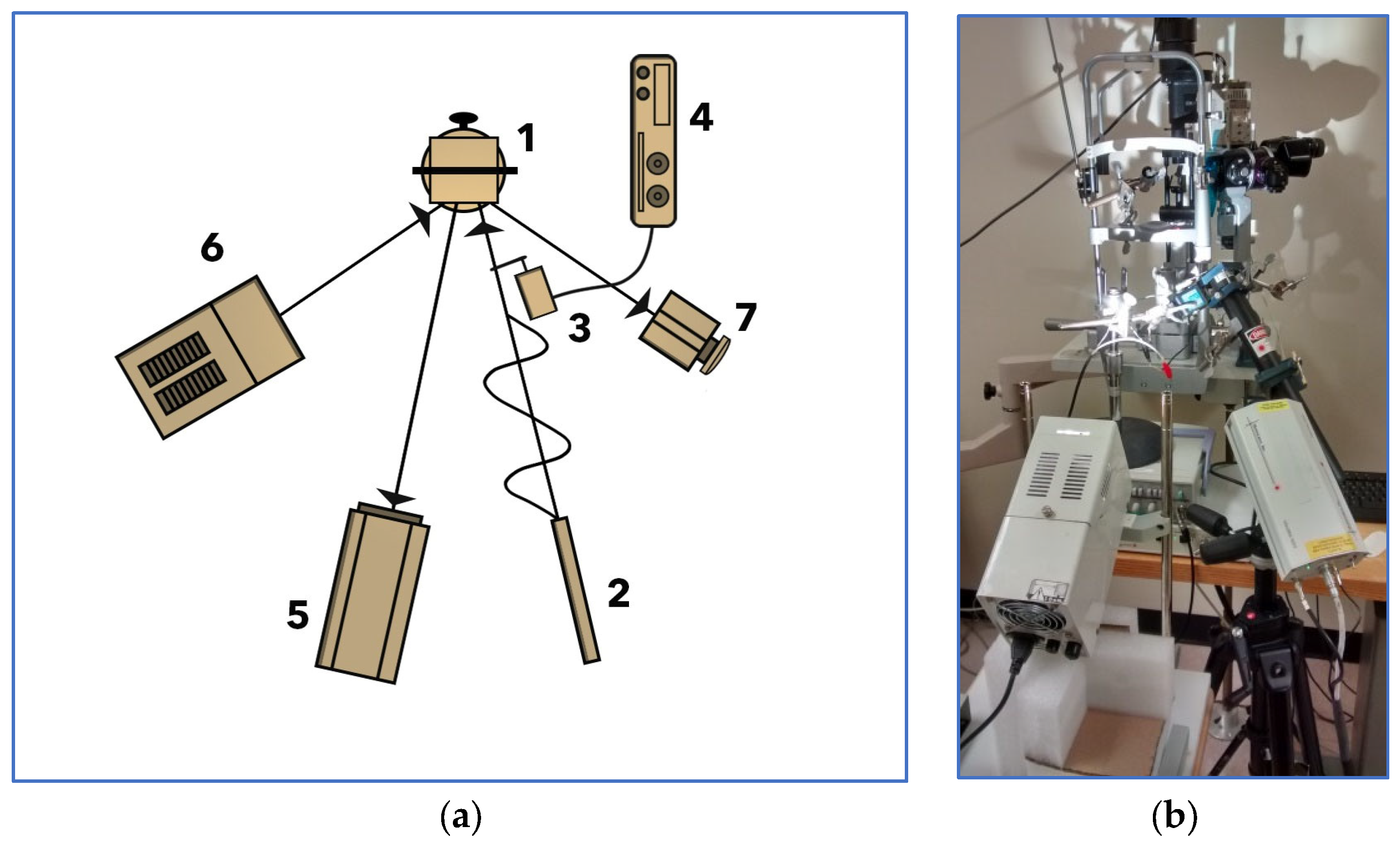
The optical setup for measuring photonic structure oscillations (
Figure 1) consists of placing the photonic structure in a metallic base (1) in the optical setup. We induced mechanical vibrations with the help of a laser (633 nm) with a power of 8.4 mW (2) and a mechanical chopper (3) driven by a function generator (4). The vibrations were measured with a Doppler vibrometer (5), and a camera (7) was video-streaming the experiment through a color analogical monitor. Videos were recorded with an IOS phone for post-processing. We used white light illumination (6) to obtain better visualization conditions.
2.2. Porous Silicon Sample Preparation
Making porous silicon (PSi) photonic crystals involves electrochemically anodizing crystalline silicon (c-Si). Highly boron-doped c-Si substrates with orientation (100) and an electrical resistivity of 0.001–0.005 Ohm cm (room temperature = 25 °C, humidity = 30%) are used to create PSi through wet electrochemical etching. An aluminum film is deposited and heated at 550 °C for 15 min in a nitrogen atmosphere to ensure good electrical contact on one side of the c-Si wafer. The silicon substrate is then anodized using an aqueous HF/ethanol/glycerol electrolyte to achieve flat interfaces. The PSi refractive index increases by decreasing the electrical current applied during the electrochemical etching. However, reducing the porosity too much can limit the subsequent contrasting high porosity layer. To address this contrast issue, an electrolyte composition of 3:7:1 is used. The HF concentration is maintained constant during etching using a peristaltic pump to circulate the electrolyte within the Teflon
TM cell. The multilayers are produced by alternating the current density applied during the electrochemical dissolution from 3 mA/cm
2 (layer 1) to 40 mA/cm
2 (layer 2), and ten periods (20 layers) are made. The current density conditions produce layers with 65% and 88% porosities, respectively. Porosity is measured using the standard gravimetrical method [
39,
40].
To obtain free-standing PSi photonic crystal foils, an anodic electropolishing current pulse (500 mA/cm2 for 2 s) is applied to lift the multilayer structure off at the end of the formation process. The PSi samples are partially oxidized at 350 °C for 10 min.
The refractive indexes of single PSi layers made under the same electrochemical conditions as the multilayers are experimentally measured to be n
1 = 1.4 and n
2 = 2.2 [
39,
40]. The refractive index was estimated from the interference fringes of the reflectance spectra of single layers on c-Si substrates [
39,
40]. Nevertheless, the experimental photonic bandgap structure fits best with refractive index values of n
1 = 1.1 and n
2 = 2. However, the refractive index and etching rate for a single layer are known to be modified in the presence of a multilayer structure, up to approximately 14% [
40]. Film thicknesses are measured using scanning electron microscopy (SEMΠ), with d
1 = 326 ± 11 nm and d
2 = 435 ± 11 nm, a period of
nm, and multilayer thickness
microns. For a more comprehensive study on Psi formation, the reader should refer to the excellent Handbook of Porous Silicon [
41].
2.3. Photonic Structure
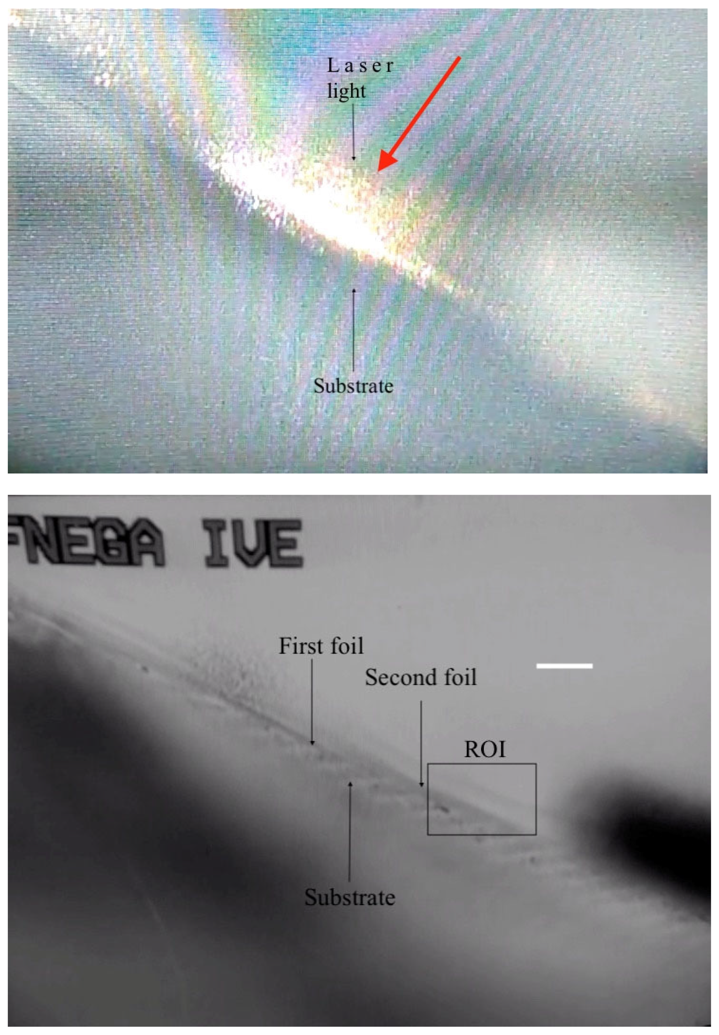
During oscillator fabrication, one issue we encountered was that the multilayer porous structure foil was not a flat membrane after being fabricated and separated from the c-Si. Due to this, the resulting membrane accumulates mechanical stress that slightly alters the original flat structure. To construct the vibrating device, two fixed porous silicon multilayer foils must be placed in mirror-like symmetry with a gap between them (see
Figure 2a). Such a configuration has the advantage of flattening both foils because the equilibrium forces for both pieces make them react against each other. We confirmed through our experimental results that this configuration worked effectively and was stable. Because the porous silicon foil is an elastic and very fragile material, it is challenging to manipulate because it is susceptible to present static electric charges. These characteristics, coupled with the poor mechanical resistance of the multilayer structure, necessitate building the device as simply as possible. We produced several prototypes with slight differences in the piece’s shape and the overlapped portion of porous silicon foils. We tested all the prototypes, which showed excellent robustness (see
Supplementary Materials).
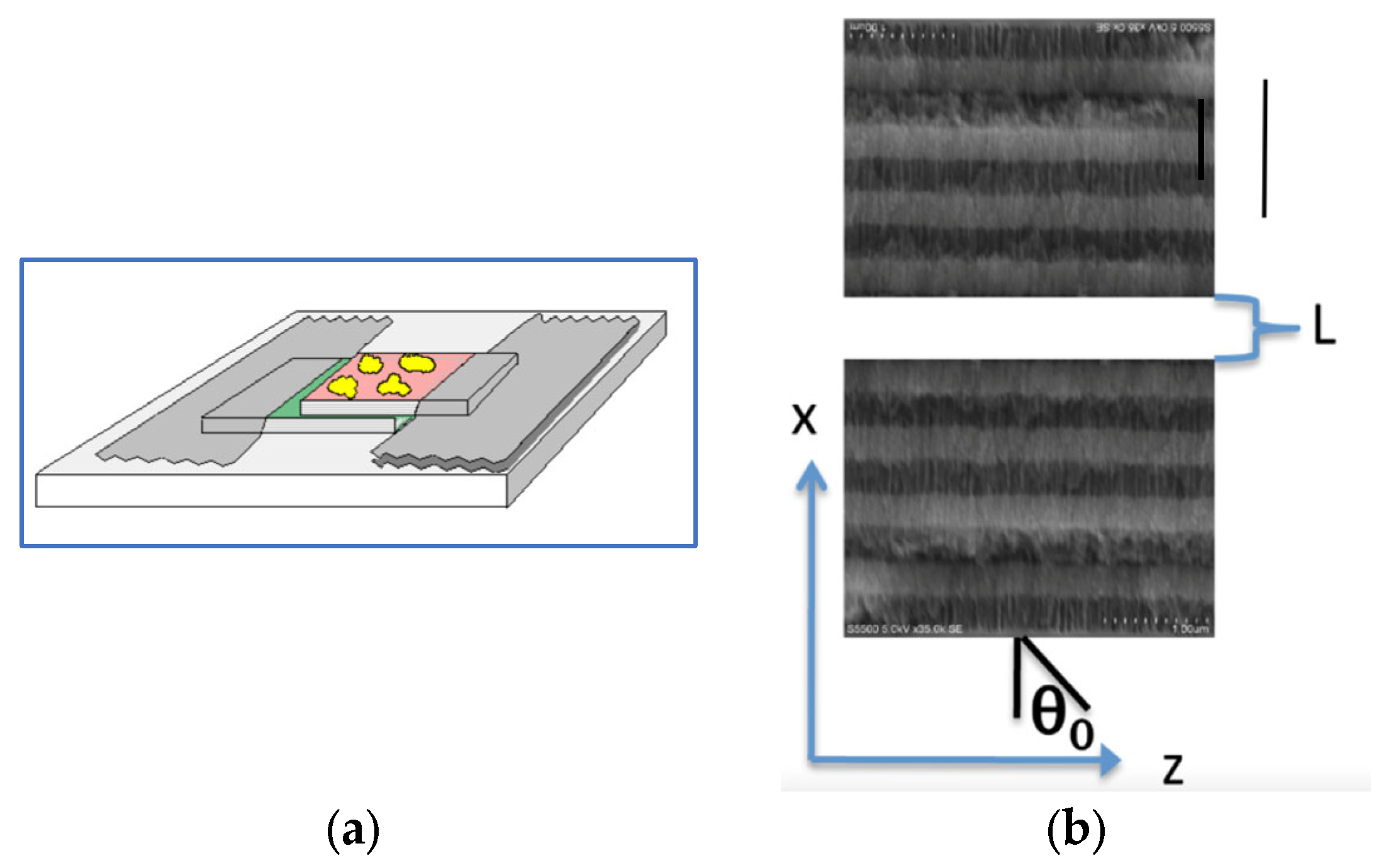
Figure 2a shows an illustration of both foils overlapping the glass substrate to create the photonic oscillator, and
Figure 2b shows a scheme of the photodyne structure of two porous silicon multilayer structures separated by a gap L (the dark regions represent low-porosity layers and the white regions represent high-porosity layers). Now, consider the structure in
Figure 2b and assume that light impinges on the off-axis direction at angle θ
0 with the electric field non-polarized. Under these conditions, we have shown in the past [
12,
13,
14,
15,
16,
17] that this photonic structure oscillates mechanically. Herein, the angle θ
0 was 35 degrees.
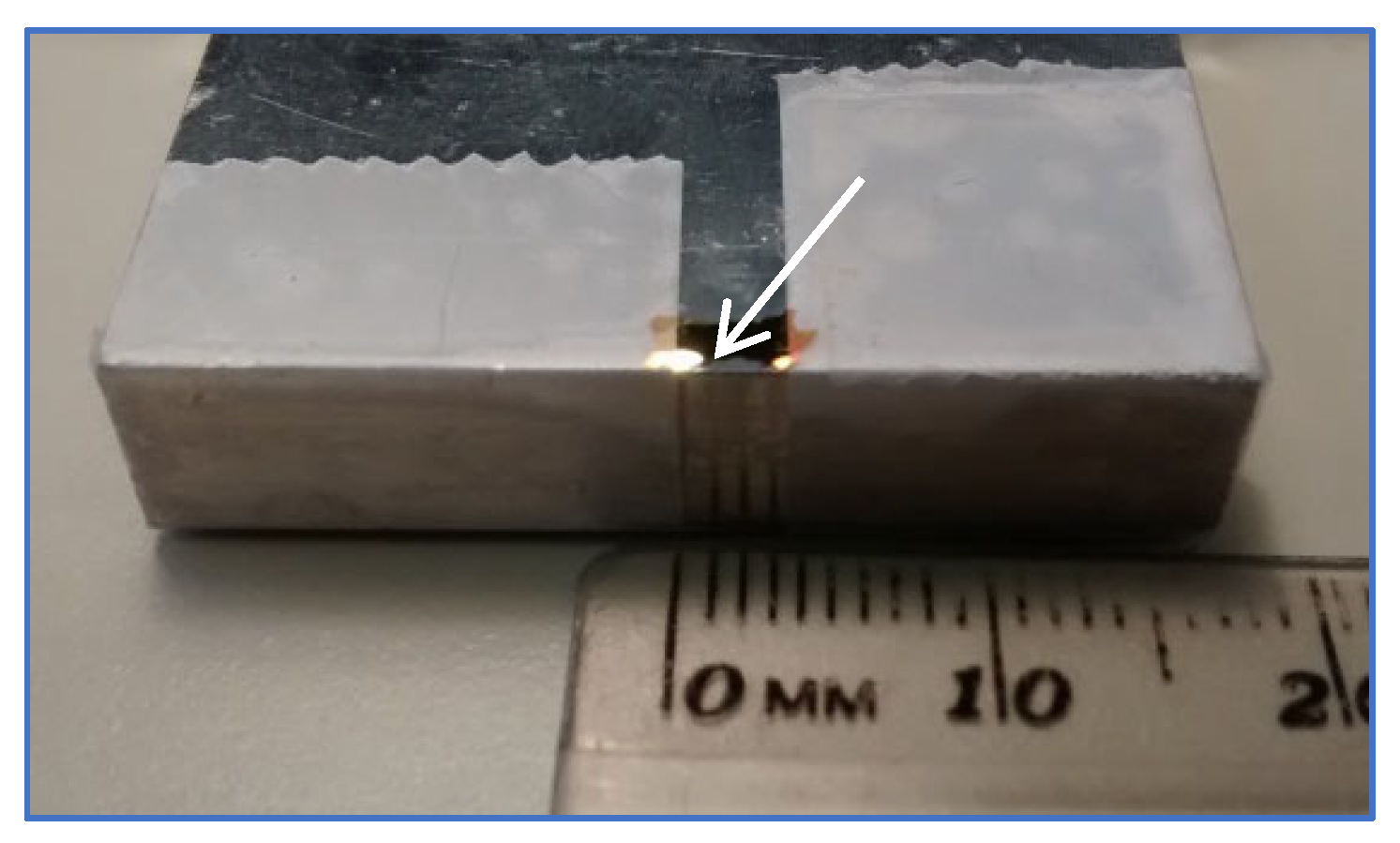
Figure 3 displays the photonic structure we used in our experiments, which is mounted on a metallic base. Each multilayer foil has a length
mm, and width
mm.
2.4. Measurement of Photonic Structure Oscillations Using a Doppler Vibrometer
An experimental setup was utilized to study the mechanical oscillations, as shown in
Figure 1. The setup involved introducing a photodyne device (1) onto a metallic base and illuminating the structure with a 633 nm laser (2). A chopper (3) modulated by a function generator (4) with an offset signal to control the duty cycle acted as a filter that switched the laser light on and off. When the light was on, an electromagnetic force was generated. The electromagnetic force generation mechanism has been amply discussed in references [
12,
13,
14,
15,
16,
17].
The electromagnetic force initiates the oscillations, captured with a highly sensitive Doppler vibration meter (metro laser model 500 v, Laguna Hills, CA, USA) (5). A laser Doppler vibrometer (LDV) is an interferometer that mixes the object beam (light reflected from the target) with a reference beam. The VibroMet 500V by MetroLaser utilizes an internal reference beam within the diode laser cavity, whereas external beam splitters are used in other commercial systems. The object beam is reflected and combined with the local reference beam at the detector to enable coherent detection. Vibrating objects scatter light, which is then Doppler shifted, altering its optical frequency based on the object’s vibration velocity.
We used white light illumination (6) to obtain a better video recorder visualization. The duty cycle was set at 50%. We forced the photodyne to move at specific frequencies between 1 Hz and 44 Hz, and we found that the system performed very stable oscillations, sometimes lasting more than 20 h, until physical damage occurred. To prevent undesirable reflection signals from entering the vibration meter, we used an infrared bandpass filter (780 nm).
2.5. Digital Movement Amplification
We utilized the Eulerian video magnification technique, which involves breaking down regular video frames into various spatial frequency bands and applying temporal filtering to reveal hidden information when amplified. This method boasts impressive capabilities and can even run in real time to observe specific temporal frequencies. Further details on this technology can be found in [
26]. The process begins by decomposing the video sequence into different spatial frequency bands and applying the same temporal filter to each band. Next, the filtered spatial bands are amplified by a given factor, added to the original signal, and collapsed to produce the output video. This method can support various applications by adjusting the temporal filter and amplification factors. For instance, [
26] utilized this system to uncover the unseen movements of a Digital SLR camera caused by the flipping mirror during a photo burst. We used non-optimized MATLAB code [
26] on a machine with a 2.8 GHz Intel Core i5 and 16 GB RAM to obtain the desired results. Each video took a few minutes to compute. This method acts like a microscope for temporal variations.
Using Eulerian video magnification to process a video involves four steps. First, choose a temporal bandpass filter (with cutoff frequencies omega low and omega high). Second, choose an amplification factor, referred to as alpha. Third, pick a spatial frequency cutoff (lambda cutoff), determining the wavelength at which alpha is attenuated. Fourth, choose how alpha is attenuated by forcing it to zero—for all lambda < lambda cutoffs—or by linearly scaling it down.
We used a CCD color video camera (KP-D50 Hitachi, Tokyo, Japan) to video stream the experiment on a color analogical monitor. The color camera has a CCD sensor that outputs RGB signals. It uses digital signal processing to regulate correction functions, producing high-quality images. Even under low-light conditions, the 410,000-pixel CCD ensures a sharp, clear image with high sensitivity and resolution. The KP-D50 camera can be remotely controlled for settings such as auto-iris, auto-white balance, backlight correction, and positive or negative picture polarity.
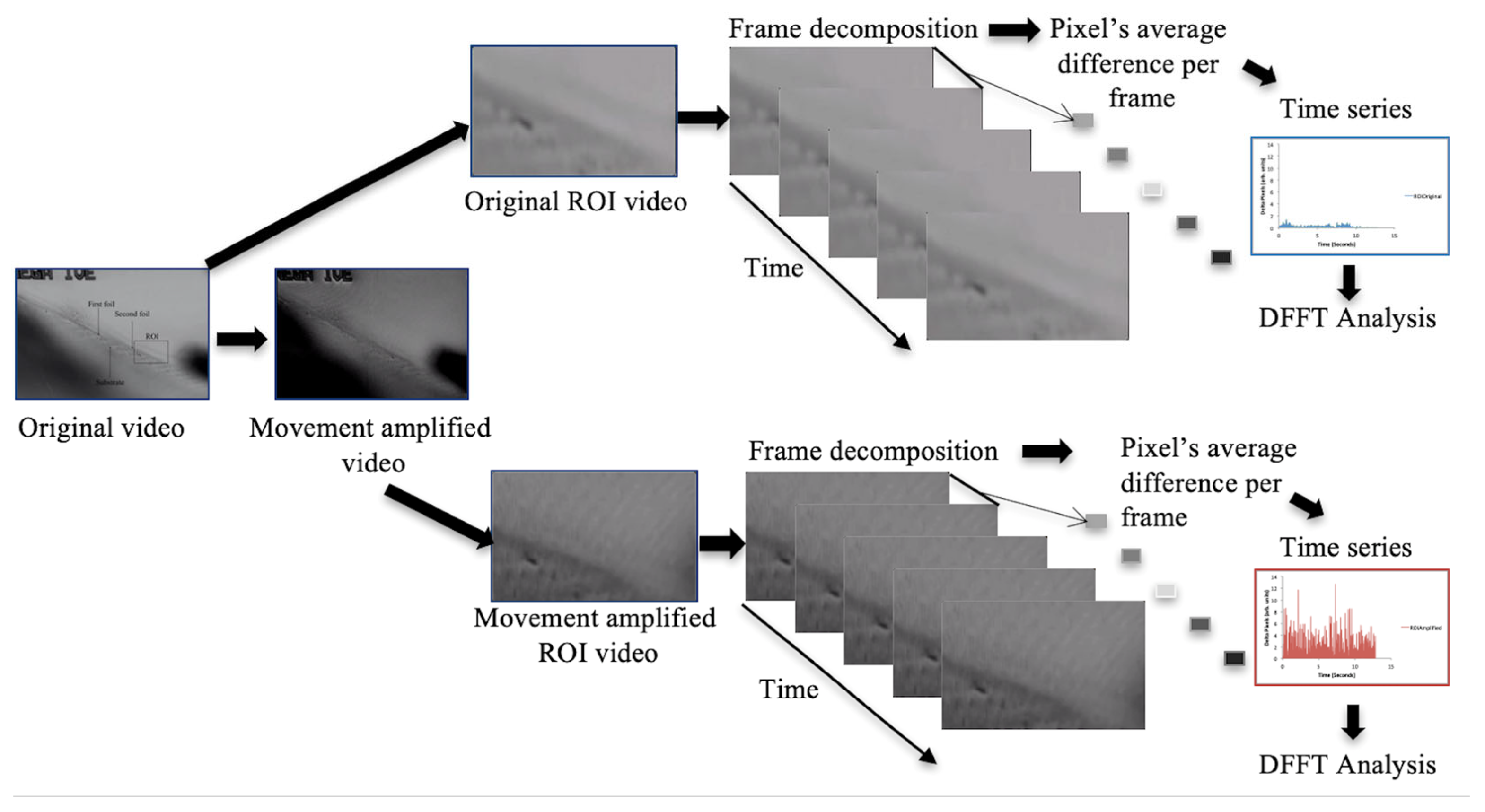
Additionally, it can be used with image processing systems or other CCTV systems as it supports external synchronization through HD and VD inputs. The video camera was coupled with a singlet lens of an 8 mm focal length (NT-45114 Edmund Optics, Barrington, IL, USA), placed 8 mm away from the sample, and an IOS phone was used to record the videos (recording at 60 fps). The first video is the original video of the oscillating photonic structure. Typically, a positive picture is displayed on the screen from the camera. However, the camera has a setting capable of displaying a positive picture when shooting a negative film illuminated from behind. Therefore, we set the picture polarity setting to negative to display the illuminated photonic structure. This action allows us to see the photonic structure, not the illumination spot that could introduce movement artifacts.
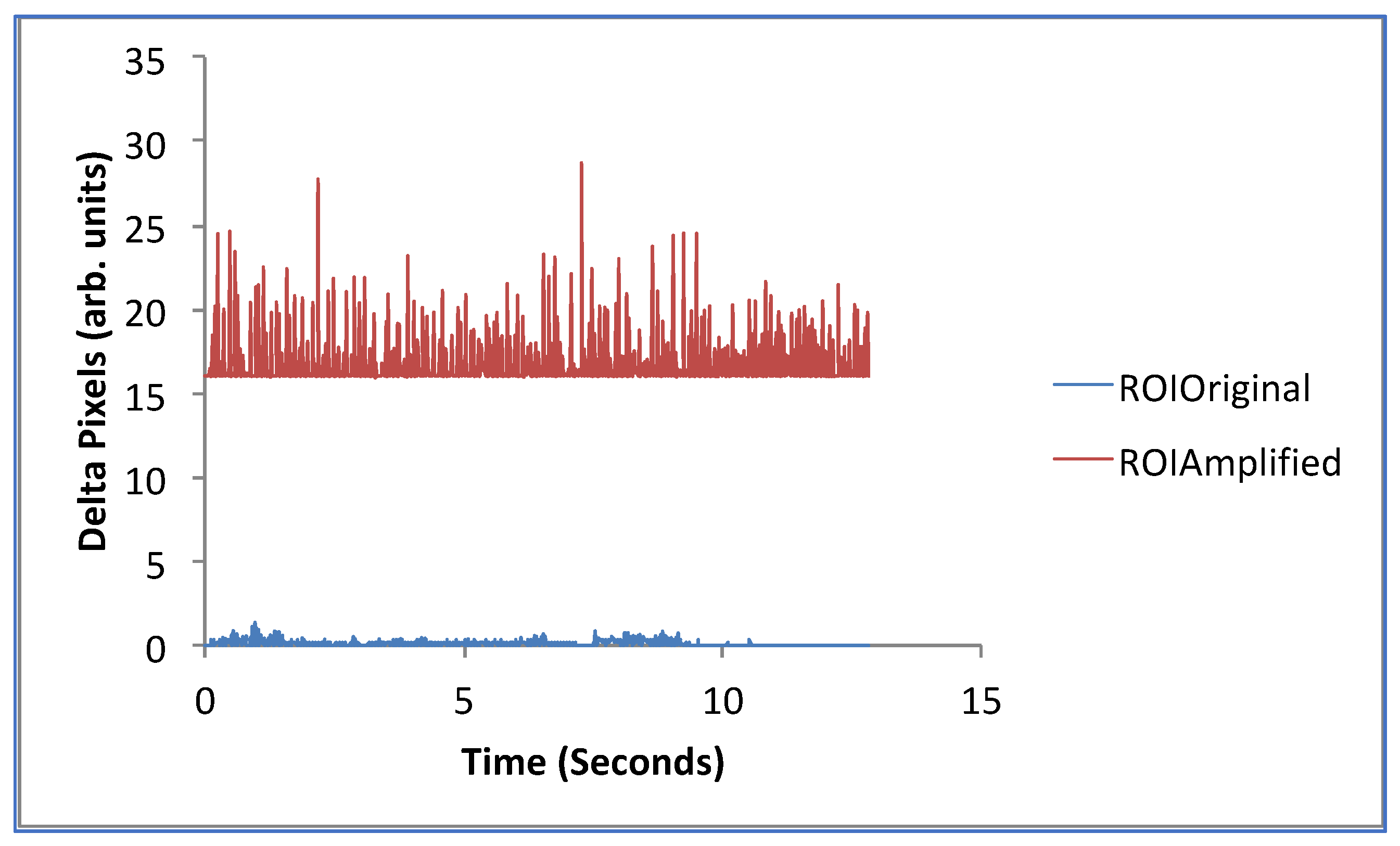
The original video, Original.mov, has a size of 839 × 553 at 59.67 fps. Then, we applied the amplification method to create a new video called Movamplification.mov, having a dimension of 649 × 393 at 58.63 fps. We found the best amplification parameters to be: magnification factor alpha = 100, low cutoff frequency = 5 Hz, high cutoff frequency = 25 Hz, and spatial frequency cutoff = 1000.
We selected the same region of interest (ROI) for these two videos. The ROI was chosen as the region that had the most precise movement image possible of the whole oscillation system. We created the videos ROIOriginal (size of 384 × 244 at 59.94 fps) and ROIMovamplification (dimension of 384 × 296 at 59.9 fps). The reader can watch these videos in the
Supplementary Materials.
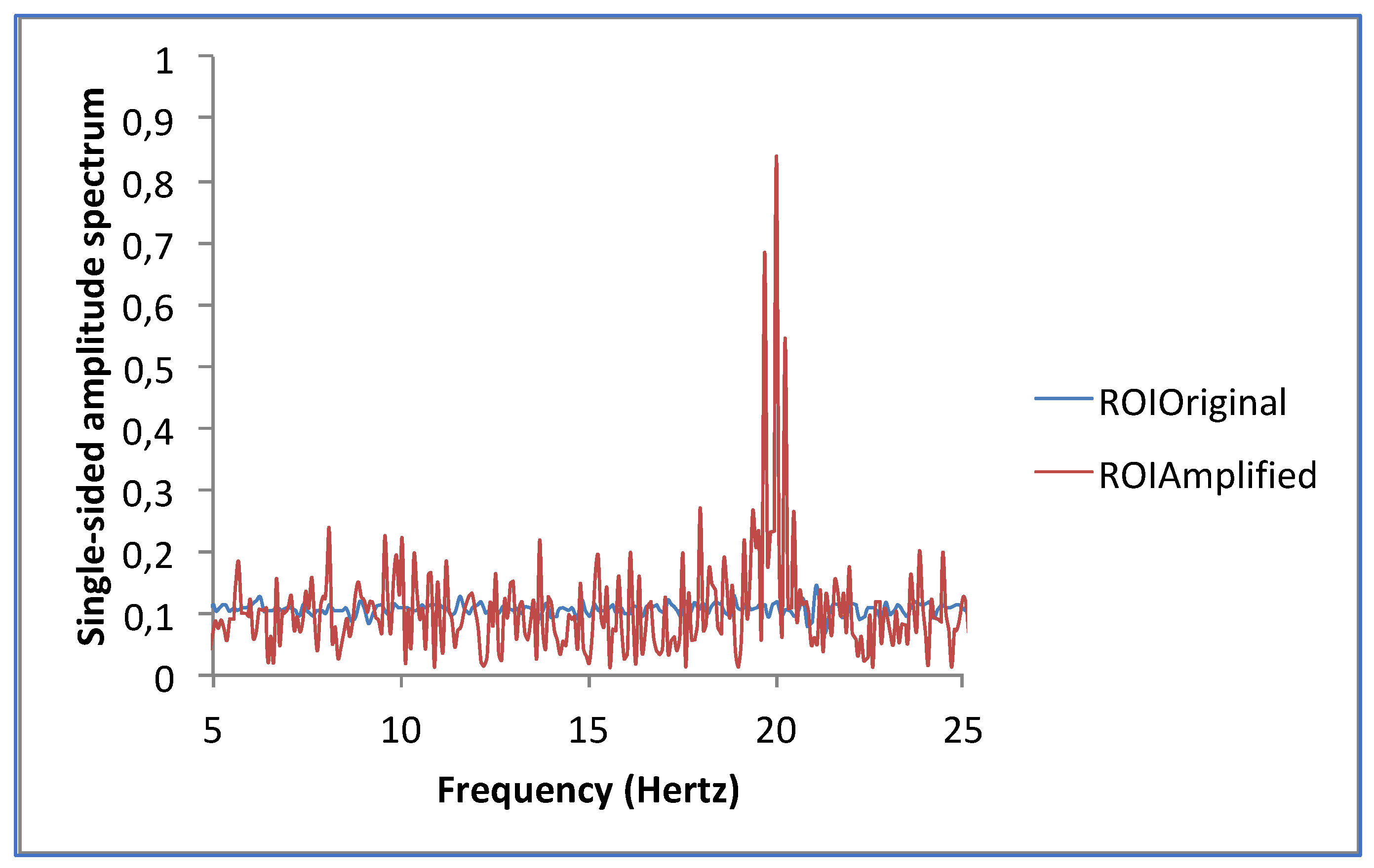
We then made two time series from both ROI videos. First, we calculated each ROI video’s pixel average in each frame and subtracted each average sequentially. Then, a Discrete Fast Fourier Transform was applied using the following parameters: number of samples = length of the time series, sampling rate = fps from the video.
Figure 4 shows all of the steps implicated in the magnification process. The velocity was obtained using the derivative of the amplitude time series. The velocity power spectral density was obtained by filtering the velocity time series using a band-pass filter with a bandwidth of 4 Hz, centered at 20 Hz.
2.6. Electromagnetic Force and Maximum Oscillation Amplitude, Velocity, and Acceleration
It can be shown theoretically [
12] that the maximum average electromagnetic force for the structure presented here occurs when the gap between foils equals
. In our present case, that gap would be around 8.6 microns. Depending on the input laser light power, the maximum electromagnetic force can be estimated as [
12]
, where
L is the light power measured in mW.
We can model our system as a simple oscillating system that can produce forced oscillations as a pendulum in a viscous frictional medium acted upon by a force of constant magnitude. The differential equation of this dynamical system is
where
,
is the foil mass,
is a damping coefficient,
is the system’s natural frequency,
defines the duty cycle (fraction of the period
where the force is on), and
is the number of cycles during which the force is on and off. So, in Equation (1),
,
, and
are known parameters from the experiment and
comes from theoretical calculations or computer simulations. For the photodyne configuration used here, the cantilever disposition is the most appropriate to apply (where the oscillation is measured on the top foil). In such a scenario, the natural frequency of the photonic system is given by
, where
is the Young’s modulus,
is the foil thickness,
is the foil length, and
is the volumetric mass density.
If the forced oscillations are closed to the auto-oscillation condition, we can estimate the maximum value for the oscillation displacement. A typical property of all auto-oscillating systems is the connection between the constant source of energy and the system, which is such that the energy given by the source varies periodically, the period of this variation being determined by the properties of the system. In this case, the period
is related to the oscillator’s frequency
as usual via
and it is related to the natural frequency and damping coefficient as
, and
, where
and
are the maximum values for the oscillation velocity and displacement, respectively, which are related through
. The maximum oscillation acceleration is given by
. The maximum oscillation displacement is then described by
2.7. FDTE Simulations
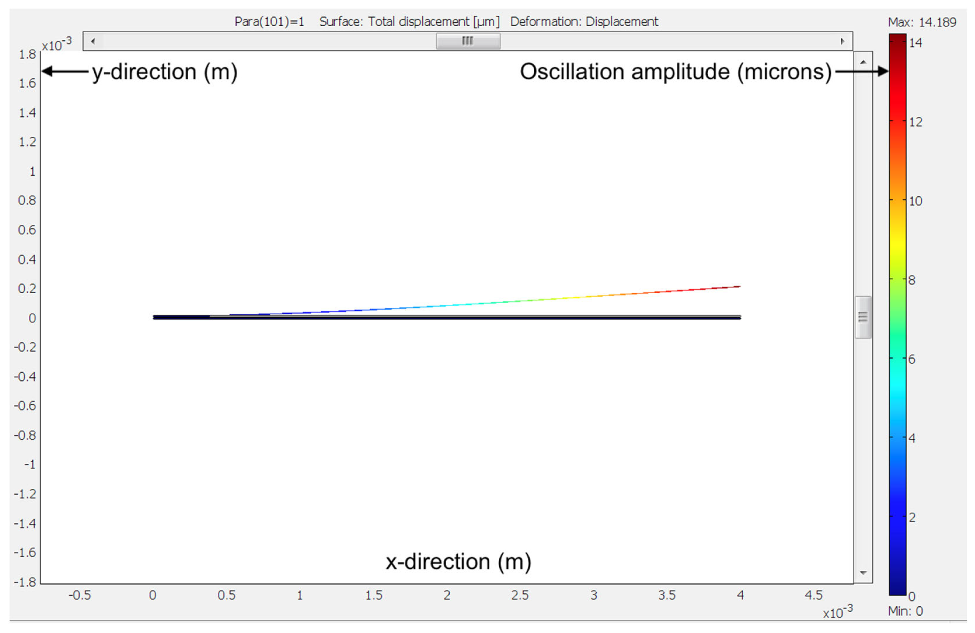
We performed full-wave finite element simulations (FEMLAB 3.1, Burlington, MA, USA). Femlab is used as simulation software for general purposes in various engineering, manufacturing, and scientific research areas. This software offers both single-physics and fully coupled multiphysics modeling capabilities, model management, and user-friendly tools that enable the creation of simulation applications. In the present work, we used the Plane Stress application mode to estimate the maximum oscillation displacement value given a maximum average electromagnetic force density. Such application is found within the Structural Mechanical Module.
First, we reproduced the geometry presented in
Figure 2. Both foils have the same geometry and mechanical properties, as shown below. An air gap of 8.6 microns separated both foils. All simulation parameters are displayed in
Table 1.
4. Discussion
The results of this proposal show the possibility of extracting mechanical vibration information from an excited photonics structure or photodyne, through analyzing a non-clear movement from a video recording, magnifying the video recording, a simple theoretical model, FDTE simulations, and applying Fourier theory for better vibration visualization.
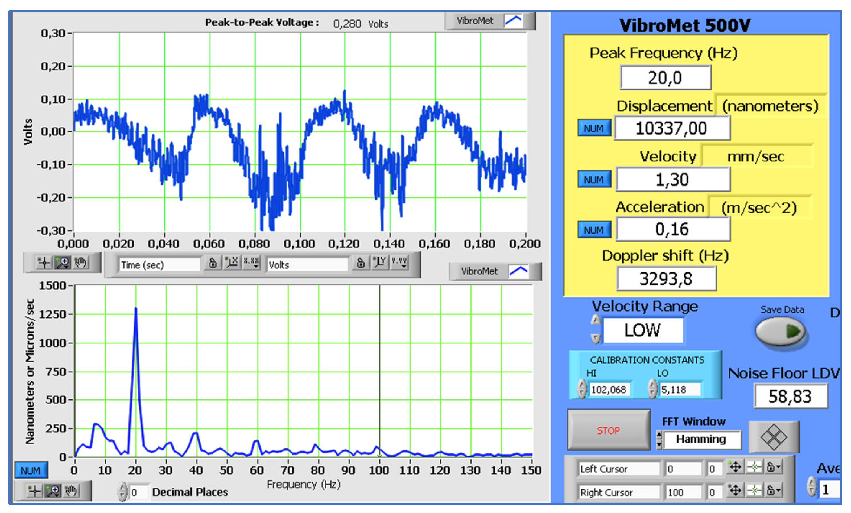
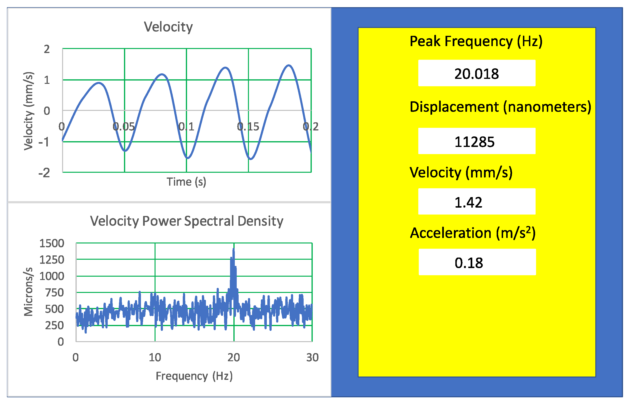
In
Figure 5, we observed the experimental oscillation results of a photodyne using a laser Doppler vibrometer. This technique gave us the following values:
microns,
mm/s, and
m/s
2.
The harmonic oscillation time series for the velocity (
Figure 5—top-left panel) suggested that we can model our system as a simple oscillating system that can produce forced oscillations as a pendulum in a viscous frictional medium acted upon by a force of constant magnitude. This model, along with the auto-oscillation condition, allows the estimation of the maximum oscillation amplitude, velocity, and acceleration. In the auto-oscillation condition, for 50% of the time, the laser light is on, and for the other 50%, it is off. Thus, the electromagnetic force is present in half of the period, and the system is moved by inertia in the other half. Consequently, most of the power is concentrated in a peak in the Fourier domain (
Figure 5—bottom-left panel). The values obtained using this theoretical model underestimated the experimental ones but are similar to the ones obtained using the laser Doppler vibrometer. For instance,
microns,
mm/s, and
m/s
2 are obtained with the theoretical approximation. The reason why these theoretical values are lower might be that the energy losses are overestimated. Experimentally, the auto-oscillation is not easy to fulfill, and any duty cycle fluctuation impacts the condition.
If the auto-oscillation is not fulfilled, the use of FDTE simulations becomes useful. These simulations tend to overestimate the values of the maximum oscillation amplitude, velocity, and acceleration. The simulated values were
microns,
mm/s, and
m/s
2 (See
Figure 9). It is important to remember that we used the maximum electromagnetic force for the simulation, but experimentally, we used only the case part of time. The force may change as a function of the gap between the foils and the angle of incidence of the light, which occurs during the oscillation period. Nevertheless, the order of magnitude is correct for the simulation and the theoretical approximation.
By using the theoretical approximation and the FDTE simulation values, we can obtain average values for the maximum oscillation amplitude, velocity, and acceleration (see
Figure 10—right panel). The averaged values were
microns,
mm/s, and
m/s
2. These average values allow us to calibrate the ROI-amplified data before calculating their power spectral density. This gives a calibrated oscillation amplitude times series, the derivative of which gives the calibrated oscillation velocity time series (
Figure 10—top-left panel). The power spectral density for the velocity is then obtained (
Figure 10—bottom-left panel). The units of the power spectral density are usually (mm/s)
2/Hz. To convert these units into microns/s, we multiply each value for the bandwidth peak at 20 Hz (approximately 2.4 Hz), calculate the square root of the result, and multiply it by 1000.
Another point to discuss is the precision and sensitivity of our method and how it compares with traditional vibration measurements, for instance, in optomechanical motions [
42]. In [
42], a spatial resolution of 0.00628 microns per pixel is presented. Such high resolution is mainly due to the CCD camera used in that work. In the present case, the camera has spatial resolutions of 9.8 microns per pixel (horizontal) and 13.05 microns per pixel (vertical). These resolutions are small compared to the ones in [
42].
Nevertheless, when there is movement, the digital amplification scheme proposed here helped increase the resolution at least 100 times (0.098 microns per pixel and 0.1305 microns per pixel). The structure ideally needs 3–4 pixels across each edge or feature for it to be robust. This means that the minimum feature resolution is 0.392 microns (horizontal) and 0.552 microns (vertical). This is more than enough for the maximum oscillation amplitude, which is ten microns. Additionally, the error relating to the work presented in [
42] for the size of levitated droplets is about 0.3142 microns (5 pixels), the same order of magnitude as the minimum feature resolution discussed above.
This study’s results demonstrate the successful application of the visualization technique. The power spectral density analysis of the mechanical oscillations in the photonic structure revealed a single peak at 20 Hz, just like the vibrometer result.
The presented work introduces a method for directly observing mechanical oscillations in photonic structures based on porous silicon nanostructures; traditionally, detecting oscillations in photonic structures involves using a vibrometer as an indirect measurement tool. However, this study reports an advancement in visualization techniques by replacing the vibrometer with the following specifications:
A CCD camera;
A digital movement amplification algorithm;
A theoretical approximation or FDTE simulations to calibrate the resulting time series amplitudes for the oscillations;
A Fourier analysis algorithm.
This innovative approach allows for a direct observation of changes in the photonic structure, providing researchers with a cost-effective means of studying oscillatory phenomena.
The method utilized in this study builds upon previous techniques for uncovering imperceptible movements in videos. By analyzing and enhancing subtle motions using temporal processing and spatial pooling, the proposed approach amplifies and visualizes the oscillatory behavior of the photonic structure. This technique has shown promise in medical monitoring and diagnosis, as well as in experimental and comparative physiology, and now in photonics.
Introducing this direct visualization technique presents a transformative development in photonics. It provides researchers with the capabilities to examine and analyze the dynamic behavior of photonic devices, and not just those based on porous silicon nanostructures.
5. Conclusions
In conclusion, the method presented here for directly observing mechanical oscillations in photonic structures based on porous silicon nanostructures represents an advancement in photonics research. It could offer valuable insights into photonic devices’ spatial and temporal dynamics and frequency responses, contributing to their design and optimization. This approach’s affordability and accessibility make it a promising tool for researchers across various photonic subdisciplines.
This write-up of our work focuses on the visualization and observation of oscillations and provides a quantitative analysis of the observed mechanical oscillations through Equations (1) and (2). Quantitative measurements of parameters such as the frequency, amplitude, and damping are also presented.
This work also compares the results obtained using direct observation with those obtained using traditional indirect measurement methods, such as vibrometry. Both sets of results are very similar and establish the accuracy and reliability of the technique revealed here.
While this new direct observation technique using a camera and digital movement amplification offers advantages in terms of cost-effectiveness and accessibility, it may have practical limitations. For example, the method may have limitations in capturing high-frequency oscillations or in situations where the amplitude of the oscillations is minimal. For this reason, it will be necessary to investigate the capability of this direct observation technique to capture higher-frequency oscillations. This could involve modifying the experimental setup or developing enhanced imaging techniques to overcome frame rates, sensitivity, or signal-to-noise ratio limitations.
In the future, we will explore the applicability of this direct observation technique to different types of photonic structures beyond porous silicon nanostructures, investigating the behavior of oscillations in other photonic systems, such as optical fibers, waveguides, or resonators. This new investigation would expand the scope of this research and uncover new insights in various areas of photonics. Future research should also develop methods to enable real-time monitoring and analysis of mechanical oscillations, that is, the integration of advanced image processing algorithms or machine learning techniques to detect and track oscillation patterns in the captured images automatically. Real-time monitoring would be particularly valuable in applications requiring rapid feedback or the control of mechanical oscillations. Finally, future studies should investigate how observing and understanding mechanical oscillations in photonic structures can contribute to developing novel devices or systems, such as sensors, actuators, or optical switches. For instance, future research could investigate how the oscillation modes change by infiltrating different chemical or biological compounds within the porous matrix of porous silicon.

 ,
, 


