
The Spatial Entropy of Confined Liquids


Department of Chemistry and Biochemistry, Wilkes University, Wilkes-Barre, PA 18766, USA
Liquids 2024, 4(1), 95-106; https://doi.org/10.3390/liquids4010004
Submission received: 18 October 2023
/
Revised: 15 December 2023
/
Accepted: 2 January 2024
/
Published: 8 January 2024
Abstract
:Molecular dynamics simulations have been used to investigate the structural changes in confined liquids. The density distribution functions for weakly and strongly interacting liquids were determined and compared to those of a non-interacting system in order to assess the impact of the entropic forces on the equilibrium state of the systems. The effect of the entropic forces was assessed by quantifying the layering on the liquid structure upon confinement. The more pronounced layering obtained for weakly interacting and non-interacting systems indicated that entropic forces are more effective in these systems where an increase in the multiplicity of states does not require a prohibitively high cost in energy.
1. Introduction
Entropic forces are dominant in condensed matter systems such as colloids, polymers, and even biological systems. These forces originate from the collective tendency of a system to maximize its entropy and without any apparent underlying potential. Consequently, they are considered “effective” or “emergent” forces of the physical system. These forces have been observed to manifest as an attractive interaction between particles in suspensions of macromolecules despite the absence of any energetic interaction between the suspended particles. Their magnitude seems to depend on the concentration of the solution and the shape and size of macromolecules and co-solutes. They have been found to have a significant effect on the phase and the structure of the solutions of macromolecules [1] and to be particularly stronger in suspensions containing charged species [2]. Depletion forces have been described in many other systems. They are considered to be a subset of a more general set of interactions known as “structural forces” [3].
An observation of the effect of entropic forces on the structure and the phase of a thermodynamic system was reported, perhaps for the first time, in 1939 [1]. It was observed that a stable dispersion of an elastomeric polymer (rubber latex) undergoes a phase separation upon mixing with certain hydrophilic colloids. No explanation of the possible mechanism for the induced phase transition was provided at that time. The earliest formal description of the underlying mechanism for the emergence of entropic forces in solutions of macromolecules was provided by Sho Asakura and Fumio Oosawa [4]. The entropic force in such systems is known as the Asakura–Oosawa depletion interaction [5].
The Asakura–Oosawa model [5] describes the behavior of a colloid suspension and presents a formal derivation of the interactions between particles in a suspension of macromolecules in the presence of co-solutes. The model derives the Asakura–Oosawa depletion interaction as an attractive force resulting from the balance between the gain of translational entropy by the small molecules in the system due to an increase in the excluded volume and the loss of translational entropy by the macromolecules due to the flocculation of the suspension [5]. The larger magnitude of the gain in translational entropy by the small colloids originates the entropic force. Since the Asakura–Oosawa model considers all the solutes hard spheres, it lacks any energetic contribution. Consequently, the effective force that is obtained is considered entirely entropic. A virial formulation of the Asakura–Oosawa effective force, recently reported [2], confirmed that the Asakura-Oosawa force, in its original formulation, involving just pair-wise interactions, is exact for small-size ratios between the small colloids and the macromolecules.
The driving force for any process taking place in a thermodynamic system is the chemical potential. In an isothermal system, the chemical potential results from changes in the Helmholtz free energy and any energetic contribution in those systems results from changes in the configurational space. These changes are entirely determined by the potential energy. Therefore, for any force to be effective in such conditions, it must be strong enough to overcome the actual interaction potential in the thermodynamic system.
In the formalism of classical statistical mechanics, the entropy (S) of a system described by coordinates q and canonical conjugate p in the phase space () is given as a function of the probability density function as [6]
where is the Boltzmann’s constant. The probability distribution function (pdf) is given by
where , T is the temperature, is the system’s energy, and
is the partition function. For a canonical ensemble, the entropy can be expressed as
where is the ensemble-average energy given by
By splitting the total energy () into kinetic () and potential () energies as
the partition function can be factorized as
where
are, respectively, the kinetic and spatial partition functions. This allows for us to write the probability distribution function as
where
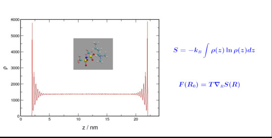
are, respectively, the kinetic and the spatial distribution functions. Spatial entropy can now be obtained integrating over the configuration phase space
and for the ensemble
where is the ensemble-average potential energy. Since the dependence on kinetic energy is factored out, the spatial entropy does not depend on the temperature, only on the spatial coordinates. Therefore, for an isothermal restructuring process, the total entropy change in the system is
The work associated with the structural changes in the system can be obtained as
This formalism can be used to analyze isothermal processes. In such processes, all changes take place in the configurational space. Consequently, the Helmholtz free energy can be expressed as
where is the change in internal potential energy and is the change in configurational entropy.
This work investigates the structural changes in confined liquids that have been attributed to entropic forces. The distribution function for non-interacting, weakly interacting, and strongly interacting systems under confinement are determined and examined in order to gain insight into the impact of entropic forces on these systems.
2. Methodology and Results
2.1. Non-Interacting Particles in a 1D Space
A one-dimensional system of non-interacting particles was generated in the following way: an arbitrary number N of pins with a finite width of were placed randomly on a rope segment of length L such that . Pins were placed with a uniform probability so that any possible arrangement was equally probable. Any position on the rope segment was considered legal for placing a pin as long as the pin did not overlap with another one or with the boundaries of the rope segment. Once all the pins were in position, the resulting probability distribution (density) function along the rope segment was determined. The density profile that was obtained is shown in Figure 1.
The density profile shown in Figure 1 is, in itself, a remarkable result. The pins are placed, along the entire segment of the rope, with a constant probability distribution and there is no interaction between them other than the fact that they are not allowed to occupy the same position on the rope. In spite of all these factors, once all the pins have been placed on the rope, the probability of finding a pin in a particular position depends on the position coordinate. In fact, the final distribution function obtained shows that the pins are attracted to the edges of the rope segment and form clusters that increase the pin density in the regions close to the edges of the rope. This effect appears to dissipate on moving away from the edges and toward the center of the rope segment. At the center of the rope segment, the distribution probability becomes uniform and it has a magnitude that is lower than that on the edges. Despite the fact that the pins are distributed along the rope segment with the uniform probability, they are more likely to be found close to the edges of the rope segment and also more likely to be close to each other rather than distributed evenly along the entire rope segment. Since there are no energetic interactions between the pins except for the case when there is overlapping, the force re-organizing the distribution of the pins along the rope segment can be considered entirely entropic.
2.2. Interacting Systems in the 3D Space
Molecular dynamics was used to model strongly and weakly interacting liquids. All simulations were performed using Gromacs-2020 [7]. Every simulated system was equilibrated in an NVT ensemble with fully periodic boundary conditions, and then equilibrated in an NPT ensemble until experimental properties were reproduced at the correct thermodynamics conditions. Argon was simulated at the liquid density at a temperature of 85 K. The ionic liquid, N-butyl-N,N,N- trimethyl ammonium bis[(trifluoromethyl) sulfonyl] imide was simulated at a temperature of 450 K. Once experimental conditions were attained, both liquids were place in between two slabs of copper and allowed equilibration. The slabs of copper were kept stationary. Periodic boundary conditions were applied in x and y directions and non-periodic conditions were used in the z direction. This was implemented using the options walls and 3dc geometry for the Particle Mesh Ewald (PME) in the Gromacs package [7].
All interaction potentials were represented using empirical force fields parameterized to reproduce the physical and chemical properties of the liquid components as well as the variety of molecular configurations found in the respective systems. These interaction potentials determine all thermodynamic, kinetic and structural properties. In particular, the force fields used to simulate argon and the ionic liquid accurately reproduce most of the thermodynamic and physical properties of both liquids. Accordingly, these potentials provide a reasonable representation of the complexities of both liquids.
2.3. Liquid Argon
Liquid argon was used as the ultimate illustration of a simple, weakly interacting liquid. This atomic liquid was modelled as a system composed of 95,000 atoms interacting through a Lennard–Jones (LJ) potential of the form
where is the distance between two Ar atoms, is the characteristic interaction energy between them and defines the length scale of the interaction potential. This is a weak, isotropic central-force potential. The reach and strength of this potential are manifested by the narrow temperature range in which Argon is a liquid. The potential parameters used for argon are those reported by Zhang [8]. The walls between which liquid argon was confined consisted of two slabs of copper, each one consisting of 7680 atoms of copper distributed in four layers of a fcc unitcell with a lattice constant of 3.615 Å and with the Cu(111) plane facing the liquid. The resulting state is shown in Figure 2.
The parameters for the Cu-Ar forcefield are shown in Table 1.
The interaction parameters between different atomic species were calculated using geometric averages as shown in Equation (17).
The value of was selected to reproduce the average range of hydrophilicity to hydrophobicity between copper and argon as prescribed by Voronov et al. [9]. That is, the well potential for Cu was set by the strength of the liquid–wall relative interaction [8]:
Calculations were performed with .
In order to keep the structure of the copper surface intact, the copper atom positions were frozen. The use of a rigid non-conducting wall is appropriate for the simulation of isothermal structural changes since production runs for the confined liquid are performed using an NVT ensemble. This ensemble is the one used in this work because it does not require re-scaling of the system’s coordinates.
The liquid was equilibrated at constant temperature (85 K) and volume for 5.0 nanoseconds with a time-step of 0.5 femtoseconds. Neighbor searching was performed every 20 steps. The cut-off algorithm with a cut-off distance of 1.2 nm was used for both electrostatic and Van der Waals interactions, and temperature coupling was performed using the V-rescale algorithm. That was followed by isobaric equilibration at 1 bar until experimental density was reproduced. Pressure coupling was performed with the Berendsen algorithm. Finally, the system was placed in between the two four-layer slabs of copper. The entire system was allowed equilibration at constant temperature for 5.0 nanoseconds. Periodic boundary conditions were used for x and y directions. The z direction was deliberately made much longer than x and y in order to obtain a good resolution for the probability density function. Once equilibrium was attained, the density profile along the z axis was determined. The probability density obtained for argon is shown in Figure 3.
The density distribution function in Figure 3 shows that the atoms in the liquid argon are attracted to the walls. Near the walls, the density of the liquid increases, and some structural re-organization is imposed on the liquid in that region. The liquid forms layers parallel to the confining walls. The density of the layers decreases as the distance from the wall increases until it reaches the bulk liquid’s density.
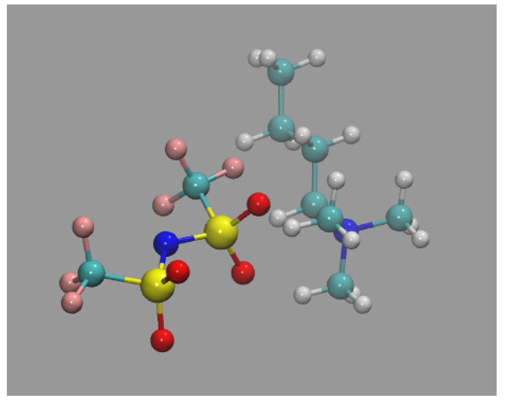
2.4. N-butyl-N,N,N-Tri Methyl Ammonium Bis[(Tri Fluoromethyl)sulfonyl] Imide (Nbatf2)
Nbatf2 is an ionic liquid with a complex molecular structure as shown in Figure 4.
This liquid has a complex, multi-component interaction potential with functional form
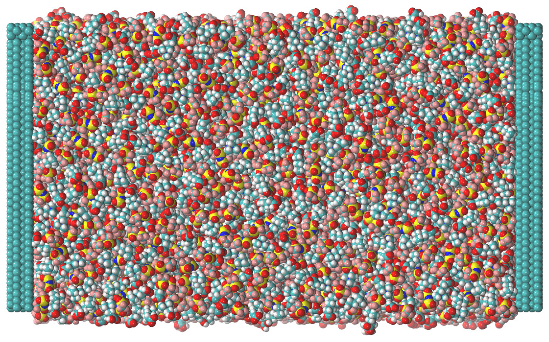
Nbatf2 was modelled as a liquid composed of 3800 molecules for a total of 155,800 atoms. The size of the system was set to minimize the statistical noise in thermodynamic properties. The length of the system along the integration coordinate (z) was set sufficiently long to ensure good numerical resolution of the probability distribution function along this axis. The force field parameters used were those reported by Maginn et al. [10]. The system was equilibrated at a temperature of 450 K and constant volume for ten nanoseconds with full periodic boundary conditions and a time-step of 0.5 femtoseconds. The V-rescale algorithm was used for temperature coupling with a time constant of 0.1 picoseconds. The Particle Mesh Ewald (PME) algorithm was used for the electrostatic interactions with a cut-off of 1.2 nm and a 96 × 96 × 192 cells reciprocal grid with a 4th-order B-spline interpolation. This was followed by equilibration in a NPT ensemble until the experimental density of the liquid was obtained. Because of the size of the system and the sluggish dynamics of the ionic liquid, this required a long simulation of 35 nanoseconds. Pressure coupling was performed using the Berendsen algorithm with a time constant coupling of 1.0 picoseconds. Once the physical properties of the liquid were reproduced, the system was placed in between two slabs of copper as it was done for liquid argon. The system was then allowed equilibration for 10 nanoseconds in a NVT ensemble. The equilibrated system is shown in Figure 5.
Once the system attained equilibrium, the density distribution function along the z axis was determined. Figure 6 shows the density distribution function obtained for confined Nbatf2.
Figure 6 shows that the molecules are attracted to the wall and form layers parallel to it with varying densities that decrease, as the distance from the wall increases, until the density matches that of the bulk liquid.
Experimental studies [11] have shown that the number and structure of the layers in confined ionic liquids depend on the molecular structure of the liquid and its interaction with the confining surfaces. The non-ionic part of the ionic liquid molecule acts as the dielectric field modulating the interaction potential of the liquid in a similar way that water modules the electrostatic interaction in electrolyte solutions. The effect of the strength of the intermolecular potential was investigated by simulating molten NaCl. In this liquid, the electrostatic interaction is at its strongest since the dielectric effect of the non-ionic part of the molecule is removed and there is no solvent. Liquid NaCl was simulated using the same exact technical options in the Gromacs package [7] that were used for Nbatf2. The simulated system consisted of 29,000 molecules of NaCl for a total of 58,000 atoms. The OPLS force field [12] parameters were used. The liquid was equilibrated at a temperature of 1030 K and a pressure of 1 bar until the reported density was obtained. Then, it was placed in between two copper slabs and allowed to equilibrate for 15 nanoseconds. After equilibration, the density distribution function along the z axis was determined. Figure 7 shows the distribution function obtained.
Figure 7 shows that confinement does not cause structural changes (e.g., layering) in the liquid structure as significant as those observed in argon and Nbatf2.
3. Discussion
All calculated distribution functions show similar behavior. Moving from the center of the region toward the walls, or to the edges in the case of the pins-on-a-rope system, the probability increases from the bulk value at the center and oscillates forming layers of increased probability in the vicinity of the walls. The increase in probability density is significantly less pronounced for the case of liquid NaCl.
The strong layering effect observed for the one-dimensional, non-interacting system of the pins on the rope has been described previously [13]. The increased probability on both edges has been attributed to an attractive entropic force created by the inaccessible space at both ends of the line. This force has been termed an “effective” force. That is, it is not generated by any underlying potential. From the point of view of pure statistics, the final configuration of the system corresponds to the distribution function of a single particle that translates into a configuration that provides the maximum accessible space for all the other particles. This configuration has the highest probability [14]. In such a configuration, each individual particle is attracted to the edges and particles are attracted to each other. Similar results have been obtained for three-dimensional systems composed of non-interacting hard spheres [15].
In the case of the interacting, three-dimensional systems of argon, nbatf2 and liquid NaCl, the distribution functions show the formation of layers, with increased probability, parallel to the confining walls. The density of the layers decreases down to the bulk density of the particular liquid when moving from the walls to the middle point between them. In spite of the significant differences in structural complexity and interaction potentials, the three systems display remarkably similar density distribution functions. All these distribution functions are also very similar to those of the one-dimensional, non-interacting system of pins on a rope. It is also noticeable that the distribution function for liquid NaCl, although it displays the same oscillations and increases probability in the vicinity of the walls as the others, the amplitude of the oscillations is much lower than that of all of the other systems. This layering effect due to confinement has been previously obtained for simple [8,15] and complex [16] liquids, and it is believed to be understood qualitatively [17]. Namely, the excluded volume at the edges of the system attracts the liquid particles increasing the density in these regions. This attraction is postulated to be an entropic force [13]. Once periodic boundary conditions are restored in all directions, the density of the entire system becomes uniform with a magnitude equal to the bulk density of the liquid.
In all the studied liquids, the distribution functions show that the atoms and molecules are attracted to the walls which is reminiscent of what is observed in the non-interacting system of pins on a rope. However, in the liquid systems, the particles exist on an energy landscape. Therefore, in order to effect change in the system, the entropic forces must overcome the energetic cost of redistributing the particles. In an isothermal process, this cost is given by the change in potential energy.
For the pins-on-the-rope system, the probability distribution shown in Figure 1 can be interpreted as a Boltzmann distribution with a potential which gives rise to an entropic force that attracts the pins to the wall and increases the probability in that region. The gradient for that force is the tendency of the system to increase its entropy [18]. Thus,
Equation (19) is the force for the macroscopic state and is the change in S with respect to the macroscopic state.
This is the only force acting in the pins-on-the-rope system since the there is no interaction potential. The magnitude of this force can be estimated from Equation (11) as
A similar calculation can be performed for all three-dimensional confined liquids, argon, nbatf2, and NaCl, by using the density distribution function calculated along the z axis and perpendicular to the plane of the confining walls. This density distribution function is calculated for slabs that are parallel to the confining walls and have a thickness of . Because of the symmetry of the systems, which have periodic boundary conditions in the x and y directions but not in the z direction, this density function is equivalent to the linear density along the z direction in the pins-on-the-rope system. On performing the calculations for the magnitude of the entropic force, using mass density () units or number density () makes no difference since the slope () of the curve is the same in both cases because the shape of the curves is identical. For unit consistency, number density units are used in Equation (20). The magnitude of the entropic force was estimated as the average slope along the entire range of the z-coordinate. Table 2 shows the magnitude of the entropic forces. For thermodynamic systems, the force was estimated using Equation (20) and the respective distribution function along the z-axis as shown in Figure 3, Figure 6 and Figure 7. The strength of this force appears similar in all the studied systems. This is mainly due to the fact that this force is the slope of the curve and small but steep changes in the distribution function can contribute substantially to its magnitude. However, the effectiveness of the force seems to diminish in the case of liquid NaCl.
Liquid argon is the thermodynamic system that more closely resembles the pins-on-the-rope system. Since its interaction potential is extremely weak, the energetic cost for the restructuring of the liquid is effectively zero. Both liquid argon and the pins-on-a-rope system adopt the most statistically favored configuration.
For systems with a strong interaction potential, the entropic force expression must be reformulated to [19]
where is the change in the Helmholtz free energy with respect to macroscopic state . represents the force in macroscopic state . A rigorous application of this equation requires the knowledge of the dependence of the internal potential energy on z (). However, an average approximate magnitude for this parameter can be obtained as the difference between the potential energy between the confined and the unconfined structures of the liquid. In isothermic processes, the contribution of internal energy comes solely from the potential energy. This change in potential energy represents the energetic cost of redistributing the particles in the system. It can be estimated as the difference in internal potential energy between the molecular configurations of the unconfined and the confined states ().
Because the nbatf2 molecule (see Figure 4) distributes the ionic charges over a large volume reducing the strength of the electrostatic interaction, liquid nbatf2 has an interaction potential with an intermediate strength between that of the potential in argon and in liquid NaCl. Restructuring (layering) of the nbatf2 system takes place but it has an energetic cost that opposes the entropic force. This is shown in Table 2. Because of the strength of the interaction potential in nbatf2, the energetic cost is affordable and nbatf2, like argon, displays significant layering upon confinement.
Although nbatf2 and NaCl are both ionic liquids, there is no dielectric screening in NaCl. Consequently, the interaction potential in NaCl is three times stronger than that in nbatf2. This strong potential increases the energetic cost of reorganizing the liquid and renders the entropic force ineffective in NaCl. This is demonstrated by the very small density oscillations observed in the probability distribution function for NaCl in Figure 7 and the very low energetic cost of the redistribution of particles (see Table 2) in the case of NaCl. The extremely low (almost zero) magnitude of this parameter indicates that there is not much redistribution of the system upon confinement due to the strong interaction potential.
Since distribution functions in the confined environment display oscillations around the bulk density, the best way to estimate the magnitude of the restructuring taking place in the liquid is to determine the standard deviation () of the normalized probability distribution function . This was calculated as
The standard deviation of the local density from the bulk density of the liquid provides a measurement of the magnitude of the layering. In order to be able to compare the standard deviations for the different density distribution functions, the functions were normalized and their zeros were set to the respective bulk value of liquid density.
Table 2 shows the standard deviation for density distribution function of the studied liquids. NaCl has the smallest deviation from bulk density. This supports the assertion that no restructuring is taking place in that liquid.
Although nbatf2 displays a seemingly small standard deviation with respect to bulk density, it is, however, thirty eight times larger than that of NaCl. This demonstrates the modulating effect that the molecular structure of nbatf2 (see Figure 4) has on the interaction potential. The covalent part of the molecule screens the ionic charges and weakens the electrostatic interaction in a similar fashion to water in ionic aqueous solutions.
4. Concluding Remarks
In a non-interacting system, the configurational state that is observed is the one with the highest probability. The multiplicity of such a state increases its probability. On flipping a coin, all sequences have the same probability, but the heterogeneous sequences (those composed of heads and tails) have a higher multiplicity than the homogeneous sequences (those composed of only heads or only tails); consequently, the heterogeneous sequences are observed more frequently because there is no penalty when switching between these two types of sequences. The randomness in these systems maximizes the effect of entropy.
In a thermodynamic system, entropy dissipates energy by creating multiple states. If the average energy of these states is lower than the internal potential energy, an energy gradient is created which, in turn, gives rise to an entropic force. If the system can be disaggregated into multiple states of different but accessible energy, entropy plays a role. This process can be aided by steric interactions and crowding effects [20], which facilitate the increase in the multiplicity of states as it can be inferred from its dominance in polymer solutions [21], colloidal suspensions [22], and even biological systems [23]. However, if the energetic cost of disaggregation is prohibitive, the increase in multiplicity does not occur.
The quantitative assessment of the layering effect upon confinement for liquids with interaction potentials of different strength shows that the restructuring of the liquid is more pronounced for weakly interacting liquids. The layering effect diminishes as the strength of the interaction potential increases. The physical systems with weak interaction potentials appear to be more susceptible to entropic forces. All this suggests that, in the case of isothermic processes, the entropic forces may only be effective in systems with weak or moderately strong interaction potentials.
Funding
This material is based upon work supported by the National Science Foundation under Grant No. 1920129.
Institutional Review Board Statement
Not applicable.
Data Availability Statement
Data are contained within the article.
Conflicts of Interest
The author declares no conflict of interest.
References
- Bondy, C. The creaming of rubber latex. Trans. Faraday Soc. 1939, 35, 1093. [Google Scholar] [CrossRef]
- Santos, A.; de Haro, M.L.; Fumara, G.; Saija, F. The effective colloid interaction in the Asakura-Oosawa model. Assessment of non-pairwise terms from the virial expansion. J. Chem. Phys. 2015, 142, 224903. [Google Scholar] [CrossRef] [PubMed]
- Trokhymchuk, A.; Henderson, D. Depletion forces in bulk and confined domains: From Asakura-Oosawa to recent statistical physics advances. Curr. Opin. Colloid Interface Sci. 2015, 20, 32–36. [Google Scholar] [CrossRef]
- Asakura, S.; Oosawa, F. On Interaction between Two Bodies Immersed in a Solution of Macromolecules. J. Chem. Phys. 1954, 22, 1255–1256. [Google Scholar] [CrossRef]
- Asakura, S.; Oosawa, F. Interaction between Particles Suspended in Solutions of Macromolecules. J. Polym. Sci. 1958, 33, 183–192. [Google Scholar] [CrossRef]
- Tolman, R.C. Principles of Statistical Mechanics; Oxford University Press: Oxford, UK, 1959; p. 539. [Google Scholar]
- Abraham, M.J.; Murtola, T.; Schlz, R.; Pall, S.; Smith, J.C.; Hess, B.; Lindahl, E. GROMACS: High performance molecular simulations through multi-level parallelism from laptops to supercomputers. SoftwareX 2015, 1, 19–25. [Google Scholar] [CrossRef]
- Yong, X.; Zhang, L.T. Investigating liquid-solid interfacial phenomena in a Couette flow at nanoscale. Phys. Rev. E 2010, 82, 056313. [Google Scholar] [CrossRef] [PubMed]
- Voronov, R.S.; Papavassiliou, D.V.; Lee, L.L. Boundary slip and wetting properties of interfaces: Correlation of the contact angle with the slip length. J. Chem. Phys. 2006, 124, 204701. [Google Scholar] [CrossRef]
- Liu, H.; Maginn, E.; Visser, A.E.; Bridges, N.J.; Fox, E.B. Thermal and Transport Properties of Six Ionic Liquids: An Experimental and Molecular Dynamics Study. Ind. Eng. Chem. Res. 2012, 51, 7242–7254. [Google Scholar] [CrossRef]
- Atkin, R.; Warr, G.G. Structure in Confined Room-Temperature Ionic Liquids. J. Phys. Chem. C 2007, 111, 5162–5168. [Google Scholar] [CrossRef]
- Jorgensen, W.L.; Maxwell, D.S.; Tirado-Rives, J. Development and Testing of the OPLS All-Atom Force Field on Conformational Energetics and Properties of Organic Liquids. J. Am. Chem. Soc. 1996, 118, 11225–11236. [Google Scholar] [CrossRef]
- Krauth, W. Statistical Mechanics: Algorithms and Computations; Oxford University Press: Oxford, UK, 2006; p. 267. [Google Scholar]
- Dill, K.A.; Bromberg, S. Molecular Driving Forces; Garland Science: New York, NY, USA, 2011; p. 81. [Google Scholar]
- Mittail, J.; Shen, V.K.; Errington, J.R.; Truskett, T.M. Confinement, entropy, and single-particle dynamics of equilibrium hard-sphere mixtures. J. Chem. Phys. 2007, 127, 154513. [Google Scholar] [CrossRef] [PubMed]
- Castejón, H.J.; Wynn, T.J.; Marcin, Z.M. Wetting and Tribological Properties of Ionic Liquids. J. Phys. Chem. B 2014, 118, 3661–3668. [Google Scholar] [CrossRef] [PubMed]
- Davies, H.T. Statistical Mechanics of Phases, Interfaces, and Thin Films; Wiley-VCH: Weinheim, Germany, 1996; p. 473. [Google Scholar]
- Sokolov, I.M. Statistical mechanics of entropic forces: Disassembling a toy. Eur. J. Phys. 2010, 31, 1353–1367. [Google Scholar] [CrossRef]
- Taylor, P.L.; Tabachnik, J. Entropic forces-making the connection between mechanics and thermodynamics in an exactly soluble model. Eur. J. Phys. 2013, 34, 729–736. [Google Scholar] [CrossRef]
- Sukenik, S.; Sapir, L.; Harries, D. Balance of enthalpy and entropy in depletion forces. Curr. Opin. Colloid Interface Sci. 2013, 18, 495–501. [Google Scholar] [CrossRef]
- Zhou, H.; Rivas, G.; Minton, A. Macromolecular crowding and confinement: Biochemical, biophysical, and potential physiological consequences. Annu. Rev. Biophys. 2008, 37, 375–397. [Google Scholar] [CrossRef]
- Arakawa, T.; Timasheff, S. The stabilization of proteins by osmolytes. Biophys. J. 1985, 47, 411–414. [Google Scholar] [CrossRef]
- Yancey, P. Organic Osmolytes as compatible, metabolic and counteracting cytoprotectans in hight osmolarity and other stresses. J. Exp. Biol. 2005, 208, 2819–2830. [Google Scholar] [CrossRef] [PubMed]
Figure 1.
Density Distribution for non-interacting particles in a 1D space.

Figure 2.
Confined Liquid Argon.

Figure 3.
Density Profile for Confined Liquid Argon.

Figure 4.
N-butyl-N,N,N-tri methyl ammonium bis[(tri fluoromethyl)sulfonyl] imide.

Figure 5.
Confined Nbatf2.

Figure 6.
Density Profile for Confined Nbatf2.

Figure 7.
Density Distribution for Liquid NaCl.


Table 1.
Cu-Ar Forcefield Parameters.
| Atom Symbol | /Å | /kJ/mol |
|---|---|---|
| Ar | 3.405 | 0.99537 |
| Cu | 2.338 | 0.2488 |
Table 2.
Calculated Properties.
| 1D System | Argon | nbatf2 | NaCl | |
|---|---|---|---|---|
| / | 0 | ≈0 | 85.44 ± 0.30 | 0.448 ± 0.152 |
| 0.1499 ± 0.0135 | 0.1475 ± 0.0204 | 0.1633 ± 0.0261 | 0.1484 ± 0.0175 | |
| 0.01662 | 0.04129 | 0.00425 | 0.00011 |
Disclaimer/Publisher’s Note: The statements, opinions and data contained in all publications are solely those of the individual author(s) and contributor(s) and not of MDPI and/or the editor(s). MDPI and/or the editor(s) disclaim responsibility for any injury to people or property resulting from any ideas, methods, instructions or products referred to in the content. |
© 2024 by the author. Licensee MDPI, Basel, Switzerland. This article is an open access article distributed under the terms and conditions of the Creative Commons Attribution (CC BY) license (https://creativecommons.org/licenses/by/4.0/).
Share and Cite
MDPI and ACS Style
Castejón, H.J. The Spatial Entropy of Confined Liquids. Liquids 2024, 4, 95-106. https://doi.org/10.3390/liquids4010004
AMA Style
Castejón HJ. The Spatial Entropy of Confined Liquids. Liquids. 2024; 4(1):95-106. https://doi.org/10.3390/liquids4010004
Chicago/Turabian StyleCastejón, Henry J. 2024. "The Spatial Entropy of Confined Liquids" Liquids 4, no. 1: 95-106. https://doi.org/10.3390/liquids4010004