Article

Development of Machine Learning Flood Model Using Artificial Neural Network (ANN) at Var River

by
Mumtaz Ahmad
1,
Md Abdullah Al Mehedi
2,
Munshi Md Shafwat Yazdan
3,* and
Raaghul Kumar
3
1
Department of Environmental Science, Brandenburg University of Technology, 03046 Cottbus, Germany
2
Department of Civil and Environmental Engineering, Villanova University, Villanova, PA 19085, USA
3
Civil & Environmental Engineering, Idaho State University, Pocatello, ID 83209, USA
*
Author to whom correspondence should be addressed.
Liquids 2022, 2(3), 147-160; https://doi.org/10.3390/liquids2030010
Submission received: 24 June 2022 / Revised: 19 July 2022 / Accepted: 25 July 2022 / Published: 1 August 2022

Abstract

:
Data-driven flow forecasting models, such as Artificial Neural Networks (ANNs), are increasingly used for operational flood warning systems. In this research, we systematically evaluate different machine learning techniques (random forest and decision tree) and compare them with classical methods of the NAM rainfall run-off model for the Vésubie River, Nice, France. The modeled network is trained and tested using discharge, precipitation, temperature, and evapotranspiration data for about four years (2011–2014). A comparative investigation is executed to assess the performance of the model by using Root Mean Squared Error (RMSE), Mean Absolute Error (MAE), and a correlation coefficient (R). According to the result, Feed Forward Neural Network (FFNN) (a type of ANN) models are less efficient than NAM models. The precision parameters correlation coefficient of ANN is 0.58 and for the NAM model is 0.76 for the validation dataset. In all machine learning models, the decision tree which performed best had a correlation coefficient of 0.99. ANN validation data prediction is good compared to the training, which is the opposite in the NAM model. ANN can be improved by fitting more input variables in the training dataset for a long period.

1. Introduction

Due to long-term global climate change, extreme weather patterns become normal, which is causing floods globally and more frequently [1,2,3]. Extreme floods can be stimulated by extreme precipitation, longer duration, close repetition of precipitations, or a combination of these [4,5,6,7,8,9,10,11,12,13,14,15,16,17,18,19]. Consequently, river engineering is growing more challenging day by day. Floods have an enormous social impact on the community and individuals, which can cause loss of human life, property damage, destruction of crops and livestock loss, and deterioration of health and migration [20,21,22,23]. It is very important to study and analyze the previous data on flooding to assess flood risk and proposed mitigation and protection measures.
The development of a model capable of identifying regions of flooding susceptibility is a critical step toward resilient flood management [24,25,26,27,28,29,30,31]. River managers must obtain discharge and water surface elevation projections for flood mitigation [32,33]. The forecast of river flow with high accuracy can be used for the economic interest of a large population in various economic sectors such as hydropower projects, irrigation, and agricultural land management, as well as taking action to avoid and reduce the potential risk of floods, and it is becoming more important for alpine areas, where a large population living downstream is reliant on river flows for agriculture land and economic activities [34,35,36]. Data-driven models, such as Artificial Neural Networks (ANNs), that are not only inexpensive but also thorough and dependable, have been widely employed in recent decades to anticipate stream and river flows [37,38,39,40,41,42,43,44,45]. Artificial Neural Networks (ANNs) algorithms are self-learning from their surroundings and making responses; they are extremely adept at dealing with nonlinear data and producing highly accurate findings and predictions. Despite the fact that some research has demonstrated that these models perform poorly during peak hydrological events. Low accomplishment from these models suggests late forecasts, namely time inaccuracy, under prediction, or both [44]. Similarly, researchers have estimated the diurnal runoff in rivers using ANNs [44,45,46]. Model-based prediction of any variable may be alarming due to several uncertainties such as inadequate or unequal input data, measurement errors, model simplification, and improper model calibration [47,48,49]. This necessitates the use of a strong model that can efficiently alter new scenarios with a variety of diverse input data and offer the finest depiction. The lack of representative input observations for training models is one of the most prominent causes of low model accuracy [50,51].
Forecasting models employ autoregressive inputs, also known as antecedent input variables, to predict real-time data. Much research has been conducted to determine whether utilizing preprocessing techniques improves model performance. To improve prediction accuracy on irregular data, ensemble-based and resampling approaches are applied. The ensemble is usually used for classification, but regression resampling is a very old approach for producing a more equally distributed target dataset for use as training data [52,53,54]. Machine learning’s two most significant techniques are regression and classification, where a regressor is used to estimate the data, and classification is simply predicted in yes/no or flooded/not flooded [55,56,57]. FFNN model techniques connect input data to output (objective or target) via a network of neurons and achieve a high level of connection between input, output, and neurons, allowing the model to reflect the system’s nonlinear behavior [58,59]. There are several Artificial Neural Network models accessible, and researchers are still determining which models should be used or are best suited to a certain situation [60,61,62,63,64,65,66,67]. For time series forecasts, one of the most popular topologies is the Feed-Forward Neural Network (FFNN), a feedforward type architecture that is based on the Perceptron neuron model [67,68,69]. From an arrangement of successive interconnected neural layers, the information spreads from the input to the output so that on the way it is abstracted by neurons [68]. Due to its comparatively less complex model structure, computational efforts, incorporation of non-linearity, and stochasticity in the prediction process, FFNN yields high performance [69].
The goal of this study is to assess the capacity of the ANN model to forecast discharge (output) by employing river flow characteristics and comparing it to conventional numerical approaches as well as other ML algorithms (e.g., random forest and decision tree). These input data are preprocessed in order to fit smoothly into the model and the rainfall-runoff (RR) model of the MIKE 11 river is used for numerical modeling, with input variables from the Vésubie River, which is part of the Var River in Nice, France.

2. Materials and Methods

2.1. Study Area

The research area is a 44.93 km sub the Vésubie River in the southeast of France at 44°04′12′′ N, 7°15′19′′ E, and elevation above sea level of 964 m. The Vésubie River is one of the Var River’s segments (together with Tinee, Upper Var, Esteron, Vésubie, and Lower Var) totaling 393.35 km2. The Vésubie has a minimum elevation of 152 m and a high height of 3001 m, with an average slope of 37.19 percent. The land-use types are mostly agricultural, forests, and a few urban sections.
The weather of the watershed is normal in winter as compared to summer; the mean temperature remains in the range of −3.1 to 26.7. Redpoint on the left of Figure 1 the Vésubie River’s rain gauge station is shown. For this segment of the river, meteorological data include daily time series of rainfall, evapotranspiration in (mm), and temperature in C. Hydrological data daily time series of runoff is collected from the Météo-France website where the data are measured at the station of “LANTOSQUE_SPAC”. The geological data 25 m resolution DEM of the Vésubie is extracted from the geo-database produced by the GIS department of Métropole Nice, Côte d’Azur using ArcMap.
The Vésubie River begins with a flow of water from the high alpine of north town Saint-Martin-Vésubie from the border of Italy, which eventually joins the Upper Var of the Var River and connects to the Var’s outflow. France’s fifth biggest city Nice is located there and frequently suffered flood hazards during the flood events because of the steep slope distributed all over the catchment, the concentration-time during the flood event became relatively short.

2.2. Data Preprocessing

The daily time series data of discharge, precipitation, temperature, and evapotranspiration is preprocessed to fit in the model for the best prediction. We found that discharge of all other three-time series had been collected for 7 years in raw file data, from 2008–2014 and discharge was only from 2011 to 2014. Consequently, all other data are trimmed and data from 2011 to 2014 are used for modeling. The gap and irregularities of the time series are also checked and as a result, all of the data are cleaned except for discharge. In discharge, there was a negative value found in May of 2013 and December 2014, which was most probably caused by gauge error. Therefore, these negative values are filled with the average values of their first three-time steps.

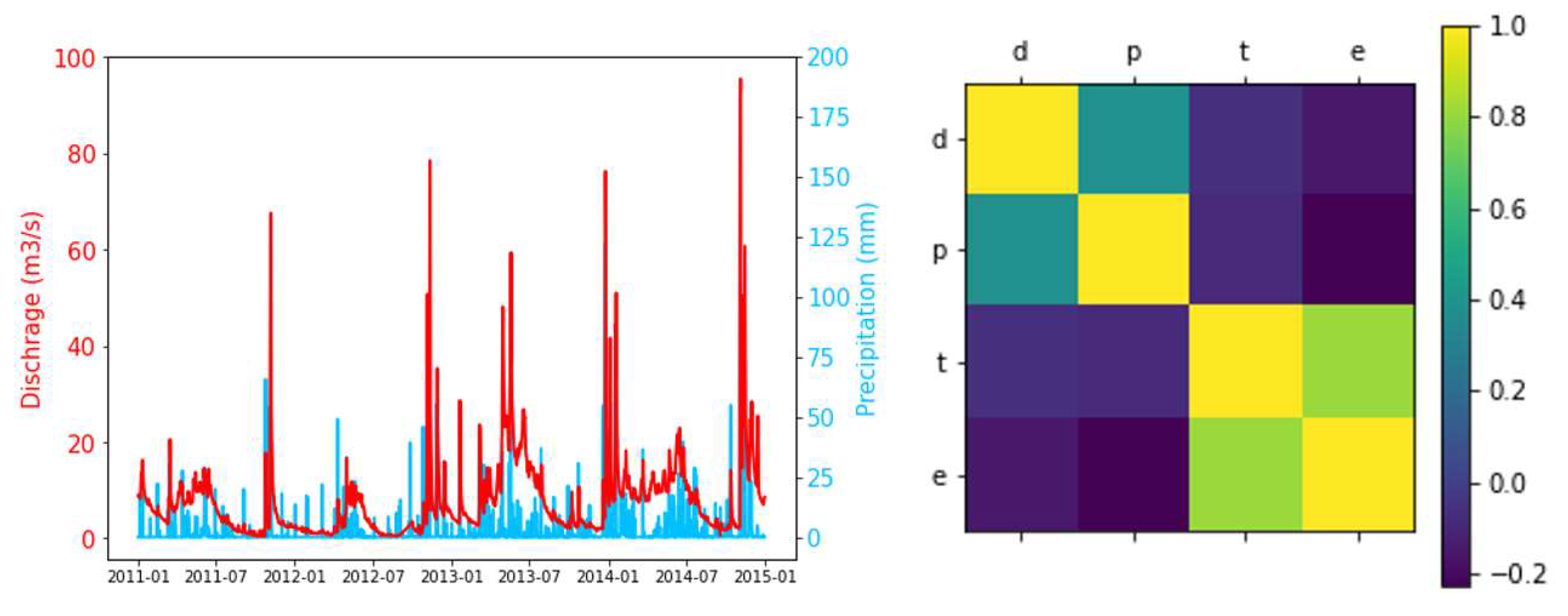
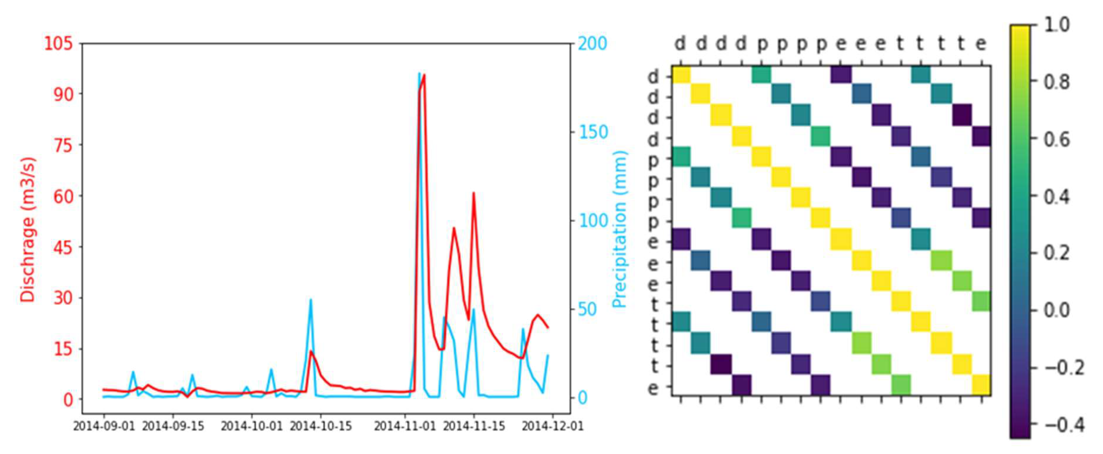
2.3. Analysis and Visualization

Based on the observation and metadata in Table 1, the mean discharge for 4 years from 2011–2014 is 7.65 m3/s, and peak discharge was recorded as 95.5 m3/s on the 5 November 2014, and the lowest was on 22 October 2011. Average precipitation is 2.88 mm and maximum precipitation was observed at 182.6 mm just one day before when maximum discharge was recorded, the minimum precipitation is 0 showing that there is no rainfall on that day. The mean temperature is 12.39 °C which is close to the average temperature of the autumn season. The minimum temperature is recorded at −3.1 on 6 February 2012 and the maximum temperature is 26.7 on 19 August 2012. The average evapotranspiration is 2.7 mm which is very near to the average precipitation, showing the strong side of MicroClimate parameters, the minimum evapotranspiration is 0.21 mm, and the maximum was 8.28.
The standard deviation of precipitation is way higher than its mean as compared to other parameters which means that it has high variation and abnormal distribution.
Figure 2 shows the daily plot of discharge, precipitation, temperature, and evapotranspiration. In the discharge plot, it is shown that there is a hike in the second last month of the year which is also similar to the precipitation plot. Temperature and evapotranspiration follow a seasonal pattern, wherein in summer they reach a peak and in winter they go down.
In Figure 3, the left side matrix plot illustrates that the correlation between daily temperature and evapotranspiration is best among all of them, at around 0.8, and after that discharge and precipitation have a good correlation, which is 0.39. The discharge versus precipitation graph shows that discharge is the outline of the precipitation like cumulative water.
In Figure 4. The left side matrix plot illustrates that the monthly correlation is better than the daily data, temperature and evapotranspiration are the best among all of them, at around 0.91, and after that discharge and precipitation have a good correlation which is 0.64. The discharge versus precipitation graph shows that the discharge follows the precipitation one step before.
Figure 5 shows the seasonal correlation of four-year data, which start from winter, summer, spring, and autumn, among all of them discharge has the best correlation with precipitation in autumn of 2014 which is 0.49. On the right side, the 2014 autumn season graph shows discharge versus precipitation, in which discharge follows the precipitation one step before.

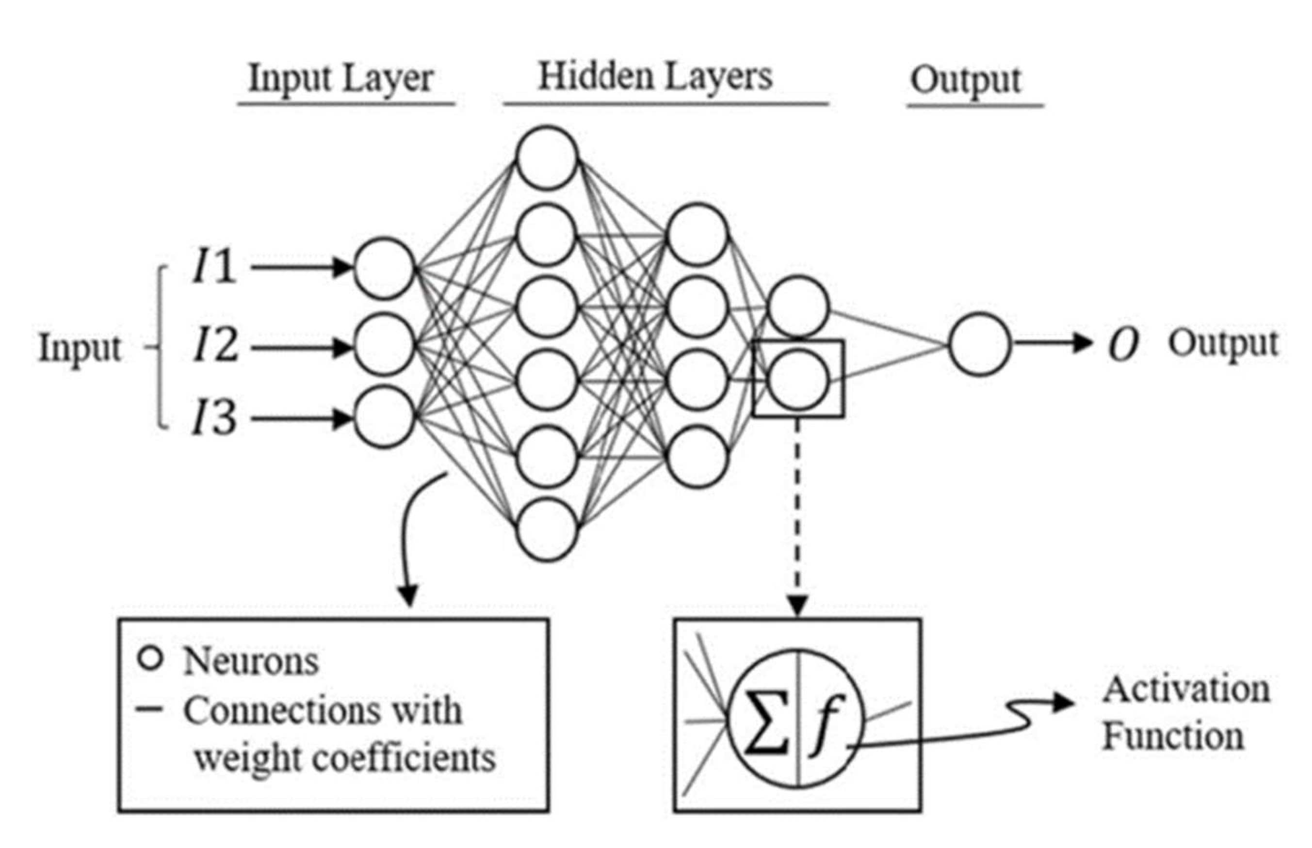
2.4. Feed-Forward Neural Network (FFNN)

A Feed-Forward Neural network (FFNN) is an ANN-based model that mimics the biological structure of the human brain and is used to understand and capture the behavior of very complex systems. The FFNN model learns and gain knowledge from the experience. This technique is particularly effective in solving dynamic and nonlinear issues such as prediction and recognition. The FFNN is one of the most extensively utilized ANN designs for the classification and regression of water resource data. FFNN networks are perceptron extensions that consist of input and output layers with some arbitrary hidden layer in between. Figure 6 depicts the FFNN model and the neuron connections.
Each hidden layer holds several neurons. Mathematically a neuron is defined as:
n e = i = 0 n x i w i + b i  
u = f n e
where x i (j = 0, …, n) are the inputs w i (j = 0, …, n) are the synaptic weights and b i is the activation threshold (bias) in the neuron potential “ne”.
Neurons are the calculating units that gather input data, analyze them, and generate output using the activation function. Although the weight connections are entirely linear, the activation function changes the output to a nonlinear form, allowing the neural network to capture the issue’s nonlinearity. The activation function used to introduce the non-linearity to the model is ReLU (Rectified Linear Unit). This function is used to introduce the non-linearity in the model. The total number of layers used to perform DNN is four including a normalized input feature layer, two hidden layers, and a linear single-output layer. The total number of weights for each trainable neuron is 4609 whereas 11 neurons are found to be non-trainable. The weights of the connections between neurons encode the FFNN’s capacity to interpret the behavior of a system. The FFNN is trained by adjusting the connection weights to replicate the behavior of the actual system. Back error propagation (BEP), the most widely used supervised training algorithm, is one way for training the neural network. BEP comprises feed-forward and reverses error propagation.

2.4.1. ANN Model

All portions of this work are carried out in Python 3.8, and the problem’s modeled network has three layers: an input layer, a hidden layer, and an output layer. The input layer is made up of three neurons that represent the problem’s input parameters, which are precipitation, temperature, and evapotranspiration. The discharge values are represented by one neuron in the output layer. In a typical ANN design, the output layer reflects the intended values of the needed prediction parameter for which the modeling is to be conducted. The output is given from the data during the training phase. However, when the model is employed as a predictor after training, the network derives these values when given with a dataset that is not a subset of training data. To prevent unnecessary model complexity, three hidden layers with different nodes are added to the network for optimum network topology. All the layers are created as Dense and combined with Sequence by using Keras and TensorFlow library. In terms of network parameters, the input and hidden layers employ a rectified ‘linear’ activation function, while the output layer uses a ‘linear’ activation function. In a neural network, the activation function describes how the weighted sum of the input is converted into an output from a node in a network layer.
Using termination criteria or early finishing, the number of training epochs is determined. This is accomplished by segmenting the calibration data into training and validation subsets.
Mean square error (MSE) is used as a Loss function, it is a method of evaluating how well the algorithm models a dataset. Good predictions have a low value of loss and a bad high loss value. Adam optimizer is used, which is the algorithm that updates the weights based on the mean square error, and accuracy is used in the matrix. All of the arguments are compiled with the model and history is fitted with the model by using the training dataset and epochs.

2.4.2. Different Machine Learning Models for Comparison

Linear Regression

Linear regression is a simple method for supervised learning which works on structural as well as time-series data. It is used for forecasting the parameter which is of continuous nature. It is the assumption that the dependency of Y on X1, X2, and Xp is linear. This relationship is denoted by the following formula:
Y = β 0 + β 1   X + ϵ

Decision Tree

A decision tree is a decision-making approach that employs a flowchart-like tree structure or is a model of decisions and all of their potential outcomes. Decision-tree algorithms are classified as supervised learning algorithms. It is applicable to both categorical and continuous output variables.

Random Forest

Random forest is another supervised machine learning technique developed by. This method is the result of the aggregation of multiple decision trees. It performs well when the number of observations is large in comparison to the number of variables. It is strong in the sense that it easily adapts to varied learning activities and efficiently provides rankings of varying priority. If the training dataset changes little, an individual decision tree can provide a significant variation in model output. Algorithm details may be found in the sources.

2.4.3. Hydrodynamic Models (NAM)

The NAM model is integrated into the MIKE model software package to create the hydrological model. The NAM model was created at the Technical University of Denmark’s Department of Hydrodynamics and Water Resources. The Danish “Nedbr–Afstrmnings Model”, which meaning precipitation-runoff-model, is abbreviated as NAM. It is currently a component of the MIKE 11 river modeling system’s rainfall-runoff (RR) model. The NAM model is a deterministic, conceptual, lumped runoff simulation model that models the rainfall-runoff process in rural catchments. It features a straightforward framework that is simple to grasp, learn, and use. NAM requires a small quantity of input data.
The data applied in this model exercise were supported by Météo-France and Métropole Nice, Côte d’Azur. The 25 m resolution DEM (MNT_25.tif) of the Vésubie catchment can be loaded by ArcMap. The model is set up in MIKE ZERO software by open rainfall-runoff (RR) parameters. The DEM of Vésubie is converted into shapefile (points) by using ArcMap and elevation zones are divided into 100 m intervals (31 classes) and the elevation zone is extracted from the map by using “Selection By Attributes”. Four-time series data are added, the model is saved, and one file is created of MIKE11 simulation. Only rainfall-runoff is active in MIKE 11 simulation and rainfall-runoff (RRPart1) is added. After setting the simulation period with a 1-day time step auto-calibration is performed.

2.5. Model Development

The input data spans four years, from 2011 to 2014. Table 2 shows the statistical properties of the data set, which comprise training and testing. Data from 2011 to 2013 are utilized for training, while data from one year are used for testing. Training data are used to construct the model, while testing data are used to evaluate the model.
To avoid variables with large values from dominating the model, normalization is conducted where each variable sits within the interval between (−1, 1). Normalization is very common and important in machine learning models because of its data sensitivity. If the data features do not look standard than the model behaves badly. Standardization leads to being more stable and less influenced by the range of variables. All data are normalized by using the following function:
z = x u s
where u is the mean and s is the standard deviation of the data samples.

Criteria for Model Performance

Root Mean Squared Error (RMSE), mean absolute error (MAE), and coefficient of determination (R) were used to assess the accuracy of the anticipated discharge. These are the most widely used for evaluating time series forecasting outcomes.
The coefficient of determination is calculated using Equation (5), which attempts to explain the link between the variables. The closer this value is to one, the better the model fits. A value larger than 0.7, on the other hand, is acceptable.
R = y ^ y 2 y y ¯ 2
where y ^ is the series’ observed value, y is the forecast value, and y ¯ is the series’ average value The variance is the difference between the expected and mean values, whereas the total variance is the difference between the original and mean values.
Equations (6) and (7) are used to determine the RMSE and MAE, where n is the number of items in the series.
R M S E = y y ^ 2 n
M A E = y y ^ n
Functions having error values near zero are the most accurate at forecasting future values, as explained more in the result.

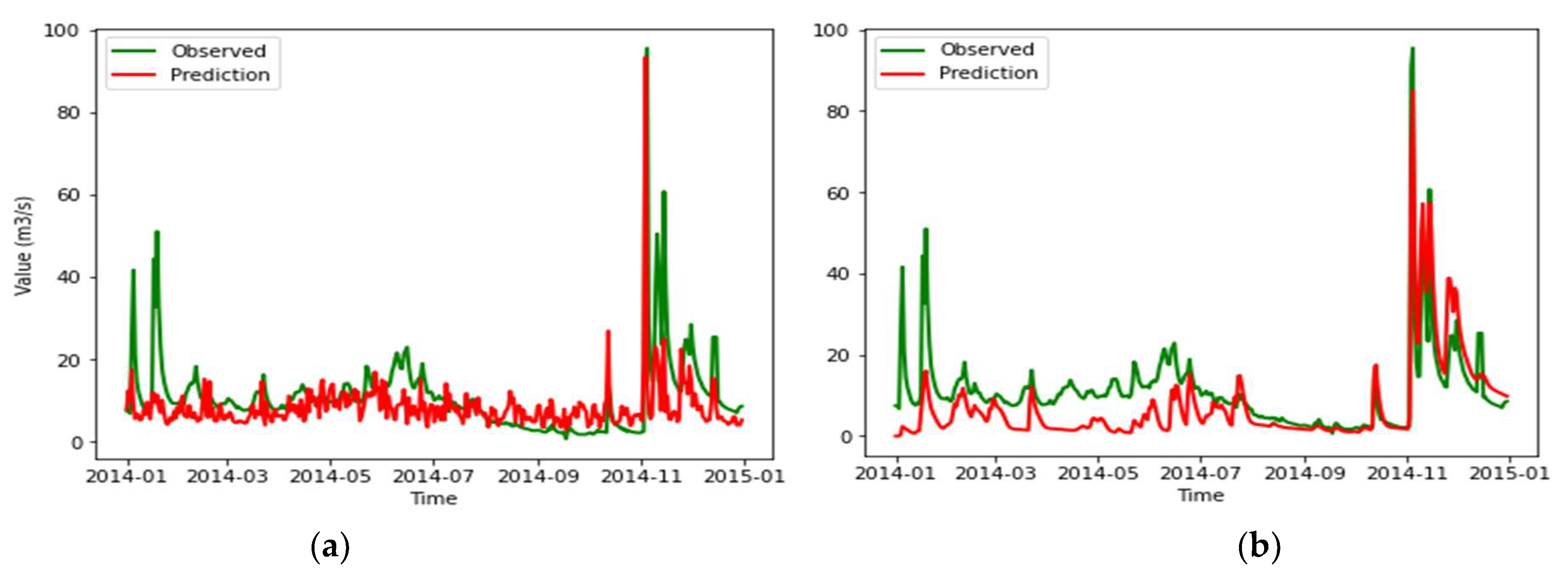
3. Results and Discussion

This section delves deeper into a comparison of performance across all approaches. The training and validation dataset results, as well as their comparison with experimental discharge levels, are shown. The performance scores of the models under consideration are computed throughout the training and testing phases. Based on the provided input architecture, Table 3 displays the performance score assessment metrics of ANN, linear regression, decision tree, random forest, and the NAM model. The performance of tree-based regressors e.g., decision tree and random forest algorithms in the training phase is better than in the testing phase (unseen data) due to the optimization and convergence through voting and bagging criteria. However, MLP offered better performance in the testing phase with unseen data minimizing/optimizing the cost function. The best R, MAE, and RMSE values for daily discharge forecasting in the decision tree algorithm for training data are 0.99, 0.03, and 0.28, respectively, while for testing NAM models projected best. The key comparison is between the ANN and NAM models, with the NAM model outperforming the others. The R, MAE, and RMSE values for the training phase are 0.78, 3.53, and 6.49, respectively, and 0.76, 5.85, and 7.94 for the testing phase. However, the MAE of ANN for testing is better than the NAM model of MAE. Table 3 shows that ANN and linear regression have comparable values in both training and testing.
The observed data and forecasted data by ANN models and NAM models are compared and given in the picture below to demonstrate the model performance accuracy on the real dataset. Low significant prediction accuracy is shown by a wide deviation from the ideal line (red line in Figure 7 for ANN). For the testing phase, NAM has a high coefficient of determinant value R = 0.76, but ANN has just 0.58. Both models anticipate peak flow well in November, but the NAM models predict better overall. Figure 8 shows scatter plots for both the ANN and NAM models to further assess prediction performance.
Furthermore, in Figure 9, the NAM model’s training phase performance is better than the testing phase performance, but the ANN model’s testing phase performance is better than the training phase. Based on the stated performance score measures, the NAM model outperforms the ANN model.
Figure 10, which depicts the entire plot of the observed and anticipated calibration and validation of both the Model ANN and the NAM model, shows that, with the exception of the November peak flood, the NAM model follows a better peak of the flood than the ANN model. It is also discovered that ANN has a higher validation efficiency than calibration when compared to the NAM model.
In a comparison of all the performed models, tree-based regressors, i.e., decision trees and random forests, have the best prediction overall, because of their low overfitting and easy interpretability. However, their performance is lower with the testing data, meaning they are outperformed by the ANN forecasting with the unseen data. Therefore, the applicability of the ANN model is much wider compared to the other ML regressors as it may perform better in several other sites. A model should be selected based on the uniqueness of the dataset for a specific location and the requirement of applying the model in the unseen area. However, by using random forest, the feature ranking of input data is also accessible. Evapotranspiration has a higher feature ranking than precipitation and temperature. The feature ranking values are 0.357037, 0.322140, and 0.320824 for evapotranspiration precipitation and temperature.

4. Conclusions

From 2011 to 2014, we investigated the machine learning methods Artificial Neural Network with NAM model or precipitation-runoff-model for forecasting the daily discharge flow of the Vésubie River in Nice, France. Between 2012–2013 and 2013–2014, the performance measurement metrics Root Mean Square Error (RMSE), Mean Absolute Error (MAE), and coefficient of determination (R) were used to input data sets for both the training and testing phases.
After partitioning the data set into training and testing and finally normalizing, the ANN model is built using Keras’ Sequence and Dense libraries and TensorFlow’s TensorFlow Library. Using meteorological, hydrological, and geological data, the NAM model is run in the MIKE11 river modeling system. Other machine learning algorithms, in addition to ANN, are used.
It was determined that the NAM model outperformed the ANN model, and the decision tree outperformed all other models of input data for the training and testing phases, respectively. The NAM model has a coefficient of determination of 0.76, however, the ANN model only has a coefficient of determination of 0.58 but evaluating the coefficient of determination of ANN is better than training. Despite the better results of the NAM model, ANN is also a dependable model for the long-term use of multiple input datasets as a feature to acquire a good result by learning all the datasets and making excellent accuracy forecasts.
While adopting the data-driven techniques, such as ANNs, researchers are still seeking solutions to the prevalent problem of poor performance with deficient input data. Furthermore, we may deduce that the work’s accuracy might be improved further by including more experimental data when training the network.

Author Contributions

Conceptualization, M.A. and M.A.A.M.; Methodology, M.A., M.A.A.M. and M.M.S.Y.; Investigation, M.A., M.A.A.M. and M.M.S.Y.; Formal Analysis, M.A.; Resources, M.A.; Data Preparation, M.A.; Writing–Original Draft Preparation, M.A.A.M., M.M.S.Y. and R.K. Writing—Review and Editing, M.A., M.M.S.Y. and R.K.; Visualization M.A., M.A.A.M. and M.M.S.Y. All authors have read and agreed to the published version of the manuscript.

Funding

This research received no external funding.

Institutional Review Board Statement

Not applicable.

Informed Consent Statement

Not applicable.

Data Availability Statement

Data collected for the study can be made available upon request from the corresponding author.

Conflicts of Interest

The authors declare no conflict of interest.

References

  1. Masson, V.; Lemonsu, A.; Hidalgo, J.; Voogt, J. Urban Climates and Climate Change. Annu. Rev. Environ. Resour. 2020, 45, 411–444. [Google Scholar] [CrossRef]
  2. Konapala, G.; Mishra, A.K.; Wada, Y.; Mann, M.E. Climate change will affect global water availability through compounding changes in seasonal precipitation and evaporation. Nat. Commun. 2020, 11, 3044. [Google Scholar] [CrossRef] [PubMed]
  3. Yao, T.; Lu, H.; Yu, Q.; Feng, W.; Xue, Y. Change and attribution of pan evaporation throughout the Qinghai-Tibet Plateau during 1979–2017 using China meteorological forcing dataset. Int. J. Clim. 2021, 42, 1445–1459. [Google Scholar] [CrossRef]
  4. Tabari, H. Climate change impact on flood and extreme precipitation increases with water availability. Sci. Rep. 2020, 10, 13768. [Google Scholar] [CrossRef] [PubMed]
  5. Teegavarapu, R.S. Floods in a Changing Climate: Extreme Precipitation; Cambridge University Press: Cambridge, UK, 2012. [Google Scholar]
  6. Alvisi, S.; Franchini, M. Fuzzy neural networks for water level and discharge forecasting with uncertainty. Environ. Model. Softw. 2011, 26, 523–537. [Google Scholar] [CrossRef]
  7. Breiman, L. Random forests. Mach. Learn. 2001, 45, 5–32. [Google Scholar] [CrossRef] [Green Version]
  8. Wu, J.S.; Han, J.; Annambhotla, S.; Bryant, S. Artificial Neural Networks for Forecasting Watershed Runoff and Stream Flows. J. Hydrol. Eng. 2005, 10, 216–222. [Google Scholar] [CrossRef]
  9. Chang, L.-C.; Amin, M.Z.M.; Yang, S.-N.; Chang, F.-J. Building ANN-Based Regional Multi-Step-Ahead Flood Inundation Forecast Models. Water 2018, 10, 1283. [Google Scholar] [CrossRef] [Green Version]
  10. Campolo, M.; Soldati, A.; Andreussi, P. Artificial neural network approach to flood forecasting in the River Arno. Hydrol. Sci. J. 2003, 48, 381–398. [Google Scholar] [CrossRef]
  11. Yazdan, M.M.S.; Kumar, R.; Leung, S.W. The Environmental and Health Impacts of Steroids and Hormones in Wastewater Effluent, as Well as Existing Removal Technologies: A Review. Ecologies 2022, 3, 206–224. [Google Scholar] [CrossRef]
  12. Yazdan, M.M.S.; Ahad, T.; Jahan, I.; Mazumder, M. Review on the Evaluation of the Impacts of Wastewater Disposal in Hydraulic Fracturing Industry in the United States. Technologies 2020, 8, 67. [Google Scholar] [CrossRef]
  13. Yazdan, M.M.S.; Rahaman, A.Z.; Noor, F.; Duti, B.M. Establishment of co-relation between remote sensing based trmm data and ground based precipitation data in north-east region of bangladesh. In Proceedings of the 2nd International Conference on Civil Engineering for Sustainable Development (ICCESD-2014), KUET, Khulna, Bangladesh, 14–16 February 2014. [Google Scholar]
  14. Al Hossain, B.M.T.; Ahmed, T.; Aktar, M.N.; Fida, M.; Khan, A.; Islam, A.S.; Yazdan, M.M.S.; Noor, F.; Rahaman, A.Z. Climate Change Impacts on Water Availability in the Meghna Basin. In Proceedings of the 5th International Conference on Water and Flood Management (ICWFM-2015), Dhaka, Bangladesh, 6–8 March 2015; pp. 6–8. [Google Scholar]
  15. Yazdan, M.; Ahad, T.; Mallick, Z.; Mallick, S.; Jahan, I.; Mazumder, M. An Overview of the Glucocorticoids’ Pathways in the Environment and Their Removal Using Conventional Wastewater Treatment Systems. Pollutants 2021, 1, 141–155. [Google Scholar] [CrossRef]
  16. Yaseen, Z.M.; El-Shafie, A.; Jaafar, O.; Afan, H.A.; Sayl, K.N. Artificial intelligence based models for stream-flow forecasting: 2000–2015. J. Hydrol. 2015, 530, 829–844. [Google Scholar] [CrossRef]
  17. Young, G.J.; Hewitt, K. Hydrology research in the upper Indus basin, Karakoram Himalaya, Pakistan. IAHS Publ. 1990, 190, 139–152. [Google Scholar]
  18. Zhu, Y.-M.; Lu, X.X.; Zhou, Y. Suspended sediment flux modeling with artificial neural network: An example of the Longchuanjiang River in the Upper Yangtze Catchment, China. Geomorphology 2007, 84, 111–125. [Google Scholar] [CrossRef]
  19. Davenport, F.V.; Diffenbaugh, N.S. Using Machine Learning to Analyze Physical Causes of Climate Change: A Case Study of U.S. Midwest Extreme Precipitation. Geophys. Res. Lett. 2021, 48, e2021GL093787. [Google Scholar] [CrossRef]
  20. Al Mehedi, A.; Yazdan, M.M.S.; Ahad, T.; Akatu, W.; Kumar, R.; Rahman, A. Quantifying Small-Scale Hyporheic Streamlines and Resident Time under Gravel-Sand Streambed Using a Coupled HEC-RAS and MIN3P Model. Eng 2022, 3, 276–300. [Google Scholar] [CrossRef]
  21. He, M.; Chen, C.; Zheng, F.; Chen, Q.; Zhang, J.; Yan, H.; Lin, Y. An efficient dynamic route optimization for urban flooding evacuation based on Cellular Automata. Comput. Environ. Urban Syst. 2021, 87, 101622. [Google Scholar] [CrossRef]
  22. Piyumi, M.; Abenayake, C.; Jayasinghe, A.; Wijegunarathna, E. Urban Flood Modeling Application: Assess the Effectiveness of Building Regulation in Coping with Urban Flooding Under Precipitation Uncertainty. Sustain. Cities Soc. 2021, 75, 103294. [Google Scholar] [CrossRef]
  23. Granata, F.; Saroli, M.; de Marinis, G.; Gargano, R. Machine learning models for spring discharge forecasting. Geofluids 2018, 2018, 8328167. [Google Scholar] [CrossRef] [Green Version]
  24. Haykin, S. Neural Networks and Learning Machines, 3rd ed.; Pearson Education: New York, NY, USA, 2009. [Google Scholar]
  25. Hasanpour Kashani, M.; Ghorbani, M.A.; Dinpazhouh, Y.; Shahmorad, S. Rainfall-Runoff simulation in the Navrood river basin using truncated volterra model and artificial neural networks. J. Watershed Manag. Res. 2016, 6, 1–10. [Google Scholar]
  26. Lee, E.H.; Kim, J.H.; Choo, Y.M.; Jo, D.J. Application of Flood Nomograph for Flood Forecasting in Urban Areas. Water 2018, 10, 53. [Google Scholar] [CrossRef] [Green Version]
  27. Breiman, L.; Culter, A.; Liaw, A.; Wiener, M. Classification and regression by random forest. R News 2002, 2, 18–22. [Google Scholar]
  28. Muthusamy, M.; Casado, M.R.; Butler, D.; Leinster, P. Understanding the effects of Digital Elevation Model resolution in urban fluvial flood modelling. J. Hydrol. 2021, 596, 126088. [Google Scholar] [CrossRef]
  29. Dewals, B.; Bruwier, M.; Pirotton, M.; Erpicum, S.; Archambeau, P. Porosity Models for Large-Scale Urban Flood Modelling: A Review. Water 2021, 13, 960. [Google Scholar] [CrossRef]
  30. Islam, A.R.M.T.; Talukdar, S.; Mahato, S.; Kundu, S.; Eibek, K.U.; Pham, Q.B.; Kuriqi, A.; Linh, N.T.T. Flood susceptibility modelling using advanced ensemble machine learning models. Geosci. Front. 2020, 12, 101075. [Google Scholar] [CrossRef]
  31. Kourtis, I.M.; Tsihrintzis, V.A.; Baltas, E. A robust approach for comparing conventional and sustainable flood mitigation measures in urban basins. J. Environ. Manag. 2020, 269, 110822. [Google Scholar] [CrossRef]
  32. Hu, M.; Zhang, X.; Li, Y.; Yang, H.; Tanaka, K. Flood mitigation performance of low impact development technologies under different storms for retrofitting an urbanized area. J. Clean. Prod. 2019, 222, 373–380. [Google Scholar] [CrossRef]
  33. Meyer, V.; Schwarze, R. The Economics and Management of Flood Risk in Germany. In Urban Water Management for Future Cities; Springer: Cham, Switzerland, 2019; pp. 473–495. [Google Scholar] [CrossRef]
  34. Guha-Sapir, D.; Santos, I.; Borde, A. (Eds.) The Economic Impacts of Natural Disasters; Oxford University Press: Oxford, UK, 2013. [Google Scholar]
  35. Da Costa, J.N.; Calka, B.; Bielecka, E. Urban Population Flood Impact Applied to a Warsaw Scenario. Resources 2021, 10, 62. [Google Scholar] [CrossRef]
  36. Rezaeianzadeh, M.; Tabari, H.; Yazdi, A.A.; Isik, S.; Kalin, L. Flood flow forecasting using ANN, ANFIS and regression models. Neural Comput. Appl. 2013, 25, 25–37. [Google Scholar] [CrossRef]
  37. Yaseen, Z.M.; El-Shafie, A.; Afan, H.A.; Hameed, M.; Mohtar, W.H.M.W.; Hussain, A. RBFNN versus FFNN for daily river flow forecasting at Johor River, Malaysia. Neural Comput. Appl. 2015, 27, 1533–1542. [Google Scholar] [CrossRef]
  38. Napolitano, G.; See, L.; Calvo, B.; Savi, F.; Heppenstall, A. A conceptual and neural network model for real-time flood forecasting of the Tiber River in Rome. Phys. Chem. Earth Parts A/B/C 2010, 35, 187–194. [Google Scholar] [CrossRef]
  39. Muñoz, P.; Orellana-Alvear, J.; Willems, P.; Célleri, R. Flash-Flood Forecasting in an Andean Mountain Catchment—Development of a Step-Wise Methodology Based on the Random Forest Algorithm. Water 2018, 10, 1519. [Google Scholar] [CrossRef] [Green Version]
  40. Nourani, V.; Baghanam, A.H.; Adamowski, J.; Kisi, O. Applications of hybrid wavelet–Artificial Intelligence models in hydrology: A review. J. Hydrol. 2014, 514, 358–377. [Google Scholar] [CrossRef]
  41. Pianosi, F.; Thi, X.Q.; Soncini-Sessa, R. Artificial Neural Networks and Multi Objective Genetic Algorithms for water resources management: An application to the Hoabinh reservoir in Vietnam. IFAC Proc. Vol. 2011, 44, 10579–10584. [Google Scholar] [CrossRef] [Green Version]
  42. Raghavendra, N.S.; Deka, P.C. Support vector machine applications in the field of hydrology: A review. Appl. Soft Comput. 2014, 19, 372–386. [Google Scholar] [CrossRef]
  43. Tokar, A.S.; Johnson, P.A. Rainfall-Runoff Modeling Using Artificial Neural Networks. J. Hydrol. Eng. 1999, 4, 232–239. [Google Scholar] [CrossRef]
  44. Gholami, V.; Sahour, H. Simulation of rainfall-runoff process using an artificial neural network (ANN) and field plots data. Arch. Meteorol. Geophys. Bioclimatol. Ser. B 2021, 147, 87–98. [Google Scholar] [CrossRef]
  45. Nourani, V.; Komasi, M.; Mano, A. A Multivariate ANN-Wavelet Approach for Rainfall–Runoff Modeling. Water Resour. Manag. 2009, 23, 2877–2894. [Google Scholar] [CrossRef]
  46. Pechlivanidis, I. Catchment scale hydrological modelling: A review of model types, calibration approaches and uncertainty analysis methods in the context of recent developments in technology and applications. Glob. NEST J. 2013, 13, 193–214. [Google Scholar] [CrossRef]
  47. Fernandez-Palomino, C.A.; Hattermann, F.F.; Krysanova, V.; Vega-Jácome, F.; Bronstert, A. Towards a more consistent eco-hydrological modelling through multi-objective calibration: A case study in the Andean Vilcanota River basin, Peru. Hydrol. Sci. J. 2020, 66, 59–74. [Google Scholar] [CrossRef]
  48. Sharma, A.; Hettiarachchi, S.; Wasko, C. Estimating design hydrologic extremes in a warming climate: Alternatives, uncertainties and the way forward. Philos. Trans. R. Soc. A 2021, 379, 20190623. [Google Scholar] [CrossRef] [PubMed]
  49. Swain, S.S.; Mishra, A.; Sahoo, B.; Chatterjee, C. Water scarcity-risk assessment in data-scarce river basins under decadal climate change using a hydrological modelling approach. J. Hydrol. 2020, 590, 125260. [Google Scholar] [CrossRef]
  50. Kauffeldt, A.; Halldin, S.; Rodhe, A.; Xu, C.-Y.; Westerberg, I.K. Disinformative data in large-scale hydrological modelling. Hydrol. Earth Syst. Sci. 2013, 17, 2845–2857. [Google Scholar] [CrossRef] [Green Version]
  51. Nohara, D.; Kitani, K.; Michihiro, Y.; Sumi, T. Decision support for preliminary release of reservoir for flood control using ECMWF medium-range ensemble rainfall forecast. In E3S Web of Conferences; EDP Sciences: Les Ulis, France, 2022; Volume 346, p. 01024. [Google Scholar] [CrossRef]
  52. Belvederesi, C.; Zaghloul, M.S.; Achari, G.; Gupta, A.; Hassan, Q.K. Modelling river flow in cold and ungauged regions: A review of the purposes, methods, and challenges. Environ. Rev. 2022, 30, 159–173. [Google Scholar] [CrossRef]
  53. Shankar, V.S.; Purti, N.; Ganta, N.; Mandal, K.K.; Singh, R.P.; Kaviarasan, T.; Satyakeerthy, T.R.; Jacob, S. Assessment of the hydrological and erosive status of South Andaman’s watersheds using drainage morphometric studies and climatic water balance model. Geocarto Int. 2022, 1–24. [Google Scholar] [CrossRef]
  54. Shahabi, H.; Shirzadi, A.; Ghaderi, K.; Omidvar, E.; Al-Ansari, N.; Clague, J.J.; Geertsema, M.; Khosravi, K.; Amini, A.; Bahrami, S.; et al. Flood Detection and Susceptibility Mapping Using Sentinel-1 Remote Sensing Data and a Machine Learning Approach: Hybrid Intelligence of Bagging Ensemble Based on K-Nearest Neighbor Classifier. Remote Sens. 2020, 12, 266. [Google Scholar] [CrossRef] [Green Version]
  55. Khan, Q.; Kalbus, E.; Zaki, N.; Mohamed, M.M. Utilization of social media in floods assessment using data mining techniques. PLoS ONE 2022, 17, e0267079. [Google Scholar] [CrossRef]
  56. Khamaiseh, S.; Al-Alaj, A.; Adnan, M.; Alomari, H.W. The Robustness of Detecting Known and Unknown DDoS Saturation Attacks in SDN via the Integration of Supervised and Semi-Supervised Classifiers. Future Internet 2022, 14, 164. [Google Scholar] [CrossRef]
  57. Rawat, S.; Saini, R.; Hatture, S.K.; Shukla, P.K. Analysis of Post-flood Impacts on Sentinel-2 Data Using Non-parametric Machine Learning Classifiers: A Case Study from Bihar Floods, Saharsa, India. In Proceedings of the International Conference on Computing in Engineering & Technology, Lonere, India, 12–13 February 2022; pp. 152–160. [Google Scholar] [CrossRef]
  58. Alatoom, Y.I.; Obaidat, T.I.A.-S. Development of pavement roughness models using Artificial Neural Network (ANN). Int. J. Pavement Eng. 2021, 1–16. [Google Scholar] [CrossRef]
  59. Tiwari, M.K.; Chatterjee, C. A new wavelet–bootstrap–ANN hybrid model for daily discharge forecasting. J. Hydroinform. 2010, 13, 500–519. [Google Scholar] [CrossRef] [Green Version]
  60. Smith, J.; Eli, R.N. Neural-network models of rainfall-runoff process. J. Water Resour. Plan. Manag. 1995, 121, 499–508. [Google Scholar] [CrossRef]
  61. Sudheer, K.P.; Nayak, P.C.; Ramasastri, K.S. Improving peak flow estimates in artificial neural network river flow models. Hydrol. Process. 2003, 17, 677–686. [Google Scholar] [CrossRef]
  62. Unal, B.; Mamak, M.; Seckin, G.; Cobaner, M. Comparison of an ANN approach with 1-D and 2-D methods for estimating discharge capacity of straight compound channels. Adv. Eng. Softw. 2010, 41, 120–129. [Google Scholar] [CrossRef]
  63. Al Mehedi, M.A.; Reichert, N.; Molkenthin, F. Sensitivity Analysis of Hyporheic Exchange to Small Scale Changes in Gravel-Sand Flumebed Using a Coupled Groundwater-Surface Water Model. In Proceedings of the Copernicus Meetings, Online, 4–8 May 2020. [Google Scholar] [CrossRef]
  64. Al Rifat, S.A.; Liu, W. Predicting future urban growth scenarios and potential urban flood exposure using Artificial Neural Network-Markov Chain model in Miami Metropolitan Area. Land Use Policy 2022, 114, 105994. [Google Scholar] [CrossRef]
  65. Wei, Y.; Xu, W.; Fan, Y.; Tasi, H.-T. Artificial neural network based predictive method for flood disaster. Comput. Ind. Eng. 2002, 42, 383–390. [Google Scholar] [CrossRef]
  66. Al Mehedi, A.; Yazdan, M.M.S. Automated Particle Tracing & Sensitivity Analysis for Residence Time in a Saturated Subsurface Media. Liquids 2022, 2, 72–84. [Google Scholar] [CrossRef]
  67. Alati, M.F.; Fortino, G.; Morales, J.; Cecilia, J.M.; Manzoni, P. Time series analysis for temperature forecasting using TinyML. In Proceedings of the 2022 IEEE 19th Annual Consumer Communications & Networking Conference (CCNC), Online, 8–11 January 2022; pp. 691–694. [Google Scholar] [CrossRef]
  68. Wang, W.-C.; Chau, K.-W.; Cheng, C.-T.; Qiu, L. A comparison of performance of several artificial intelligence methods for forecasting monthly discharge time series. J. Hydrol. 2009, 374, 294–306. [Google Scholar] [CrossRef] [Green Version]
  69. Hussain, D.; Hussain, T.; Khan, A.A.; Naqvi, S.A.A.; Jamil, A. A deep learning approach for hydrological time-series prediction: A case study of Gilgit river basin. Earth Sci. Inform. 2020, 13, 915–927. [Google Scholar] [CrossRef]
Figure 1. Var River Basin in French Mediterranean Alps and Vésubie River.
Liquids 02 00010 g001
Figure 2. Daily plot of Discharge, Precipitation, Temperature, and Evapotranspiration.
Liquids 02 00010 g002
Figure 3. Daily Discharge vs. Precipitation and Correlation Matrix.
Liquids 02 00010 g003
Figure 4. Monthly Discharge vs. Precipitation and Correlation Matrix.
Liquids 02 00010 g004
Figure 5. Discharge vs. Precipitation Autumn Season and Seasonal Correlation Matrix.
Liquids 02 00010 g005
Figure 6. ANN model and the connections between the neurons.
Liquids 02 00010 g006
Figure 7. (a) Validation of ANN, (b) NAM model.
Liquids 02 00010 g007
Figure 8. Scatter plot of (a) ANN, (b) NAM model.
Liquids 02 00010 g008
Figure 9. (a) Training ANN and NAM model, (b) Scatter Plot.
Liquids 02 00010 g009
Figure 10. (a) ANN full plot, (b) NAM full plot.
Liquids 02 00010 g010
Table 1. Meta Data.
Table 1. Meta Data.
ParametersMeanStdMaximumMinimum
Discharge (m3/s)7.658.4895.50.43
Precipitation (mm)2.889.64182.50
Temperature (°C)12.396.5226.7−3.1
Evapotranspiration (mm)2.71.738.280.21
Table 2. Data splitting training and test results.
PartitionPeriodNo. of Record
Training2011–20131096
Testing2013–2014365
Complete2011–20141461
Table 3. Model Performance in Discharge Prediction.
ModelsTraining/Calibration DataTest/Validation Data
RMAERMSERMAERMSE
ANN0.474.226.680.585.689.10
Linear Regression0.394.677.160.486.169.71
Decision Tree0.990.030.280.327.6111.42
Random Forest0.941.762.940.436.319.79
NAM Model0.783.535.490.765.857.94
Publisher’s Note: MDPI stays neutral with regard to jurisdictional claims in published maps and institutional affiliations.

