

The Optimal Size of a Heterogeneous Air Taxi Fleet in Advanced Air Mobility: A Traffic Demand and Flight Scheduling Approach


Abstract
:1. Introduction
- The complexity of the design of air taxis, involving modern battery resp. fuel cell technology and charging management within very limited space, including certification aspects;
- Airspace management in (congested) urban environments requiring advanced technologies to overcome safety concerns;
- Infrastructure development, such as the construction of landing and takeoff areas and charging stations (‘vertiports’) in potentially downtown urban areas with significantly limited space;
- Regulatory and legal challenges pertaining to air traffic management, privacy, environmental impact, and noise abatement;
- Concerns related to a potential societal shift, requiring coordination and cooperation among various stakeholders.
2. State-of-the-Art
2.1. Demand Forecast Modeling
2.2. Operational Aspects of Air Taxis
2.2.1. Air Taxi Categories
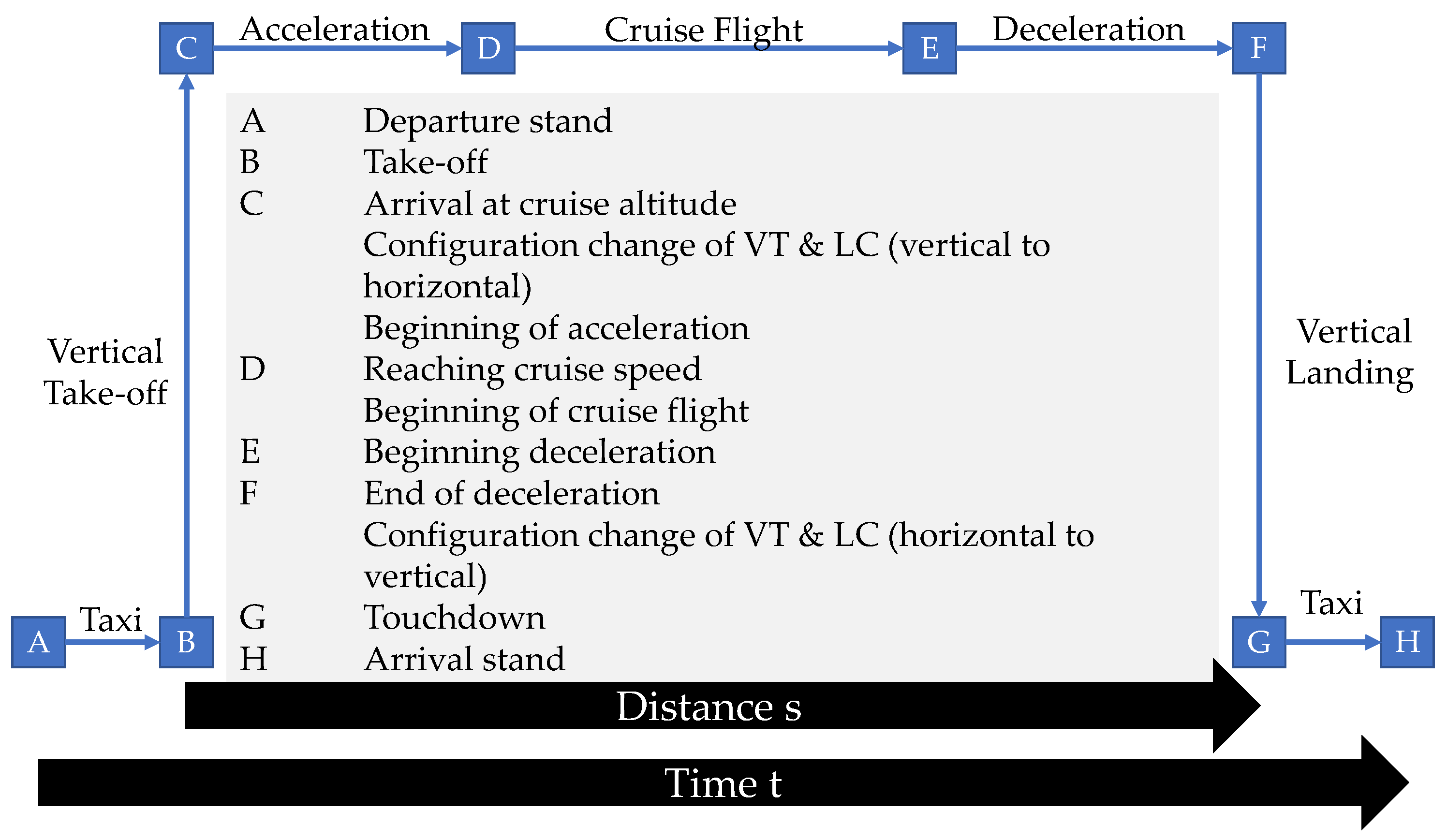
2.2.2. AAM Flight Mission Profile
2.2.3. Turnaround Procedures
2.3. Vehicle Fleet Sizing Problems
3. Case Study and Air Taxi Flight Performance
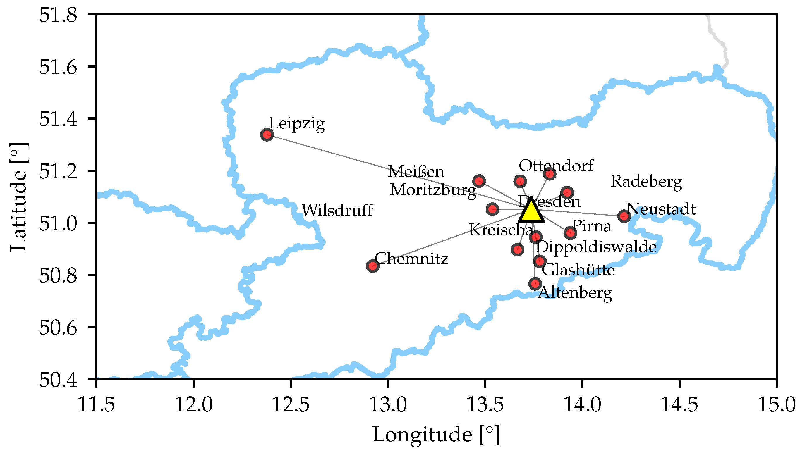
3.1. Case Study, Network and Demand for Trips
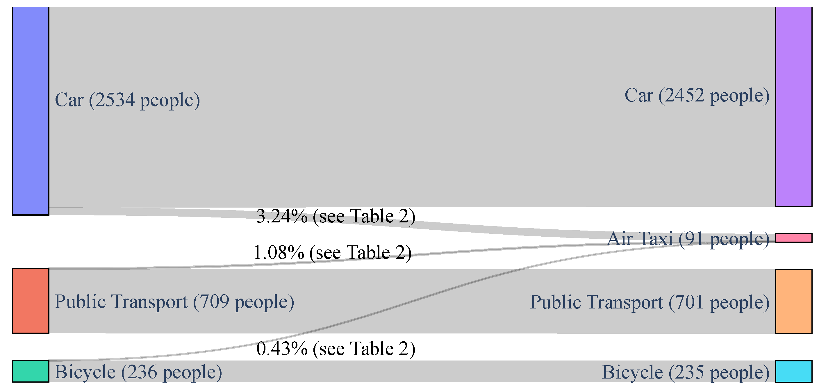
3.2. Air Taxi Travel Demand
- Bicycle trips typically involve shorter distances, characterized by very low financial outlay (purchase and maintenance costs for a bicycle). In this context, the motivation for using an air taxi could be driven by factors such as the fun factor or personal interests in technology [29].
- Public transport generally serves medium to long distances and travel times. Users in this category typically exhibit high price sensitivity, accepting longer travel times for a lower price compared to individual transport options. Here, the fun factor and potential technology interests could be influential in choosing an air taxi for sporadic trips.
- Trips covered by individual transport (e.g., cars) are also characterized by medium to long distances, resulting in a moderate willingness to pay. Users in this category accept higher operating costs for a car (purchase, fuel, maintenance, insurance) in exchange for time savings and individuality compared to public transport.
- Car users: 15%.
- Public transport users: 5%.
- Bicycle users: 2%.
3.3. Air Taxi Flight Performance
3.3.1. Taxi
3.3.2. Vertical Take-Off
3.3.3. Transition
3.3.4. Cruise
3.3.5. Vertical Landing
3.3.6. Energy Requirement
3.3.7. Range
4. Flight Scheduling and Aircraft Assignment Model
- Variables: flight schedule (departure and arrival times) with integrated air taxi allocation: which air taxi is assigned to which flight.
- Logical and valid flight schedule: no overlapping flights for an air taxi, sufficient turnaround time, time for repositioning, and a sufficient remaining battery energy level for the subsequent flight.
- Always sufficient available space at vertiports, along with immediately accessible and uninterrupted battery charging facilitated by the provided power supply. Upon arrival at the vertiport, passengers are ready for departure, thus no delays are anticipated.
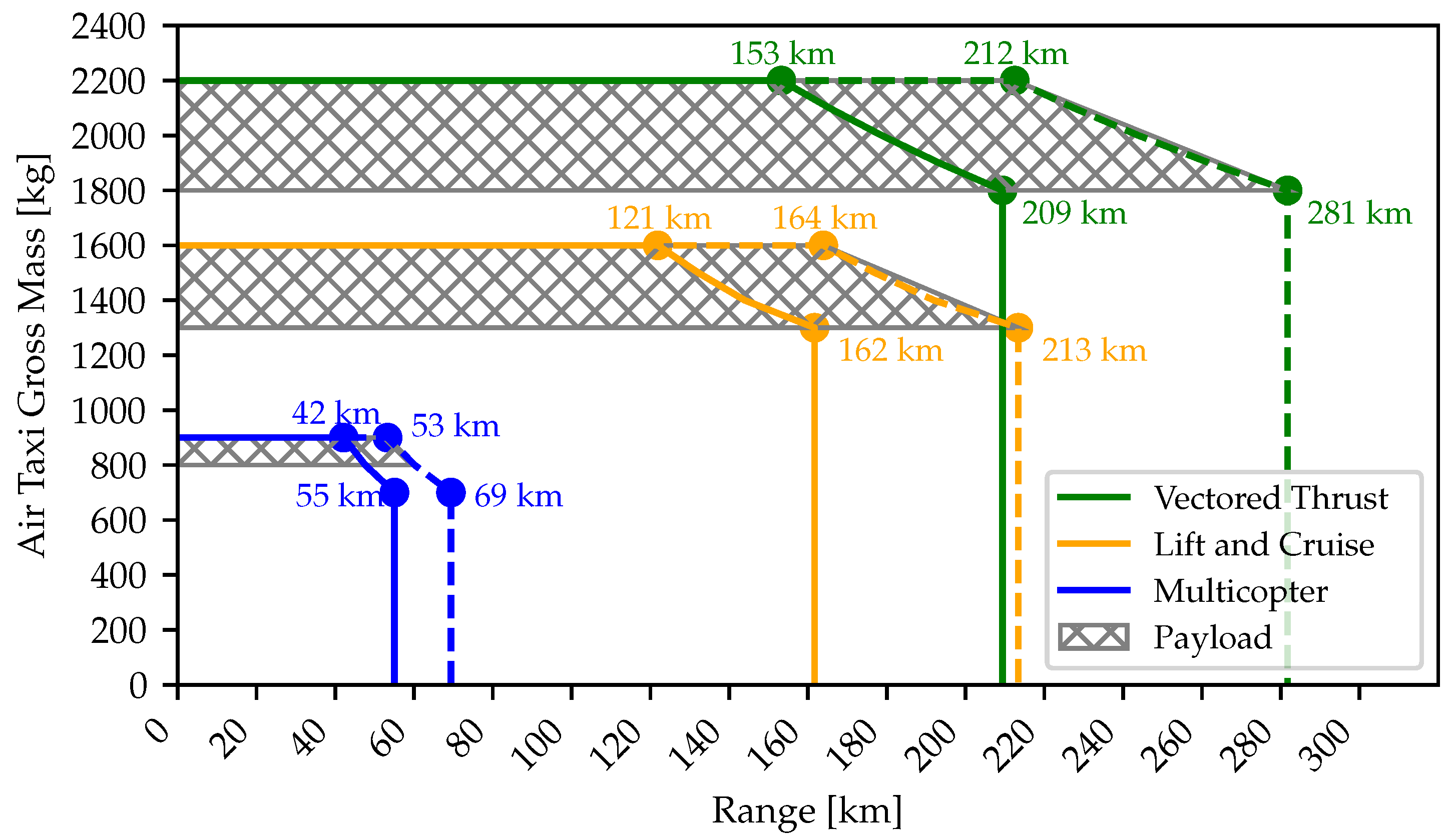
- Route restrictions exist by air taxi range and capacity (refer later in the text to the corresponding parameters depicted in Figure 9).
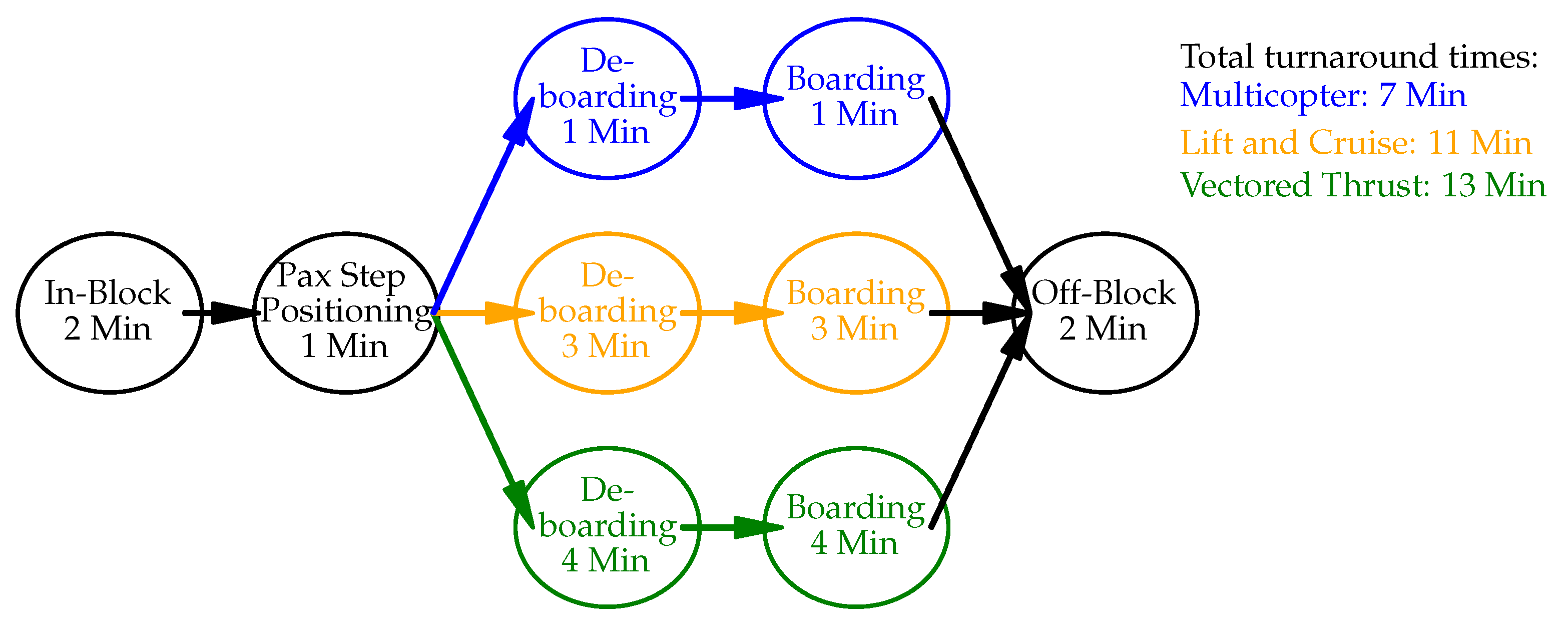
- A standard ground time is estimated, which is used to prepare the aircraft for the flight and allows for passenger boarding and deboarding (later in text in Figure 10). This time can be utilized for battery charging.
- Reliable air taxis without failures; no maintenance units due to extended planning horizon, can be abstracted via allocated time slots per air taxi.
- No new incoming requests are allowed into the system; otherwise, the calculation must be restarted.
4.1. Mathematical Formulation
| Sets: | ||
| set of flights with depot | ||
| set of flights | ||
| set of air taxi | ||
| set of arcs | ||
| Parameters: | ||
| edge cost, ground event | ||
| node cost, flight event | ||
| cost rate arrival delay | ||
| 1 if flight j can be a successor of i, | ||
| 0 otherwise | ||
| 1 if flight j can be served by vehicle k, | ||
| 0 otherwise | ||
| flight time of i with k | ||
| ground time between i and j | ||
| fix cost for using vehicle k | ||
| , | open/close fix time window | |
| , | open/close soft time window | |
| battery charging performance | ||
| battery capacity of vehicle k | ||
| M | BigM, very large number | |
| Variables: | ||
| binary variable: 1 if flights i and j are served | ||
| by vehicle k in this order, and 0 otherwise | ||
| arrival delay of flight i | ||
| start time of flight | ||
| end time of flight | ||
| time vehicle k returned to depot | ||
| help variable for delay | ||
| wait time before serving flight j | ||
| battery status of vehicle k before charging in i | ||
| battery charge of vehicle k before departure of i | ||
4.2. Heuristic Solver
| Algorithm 1 Algorithm to calculate the score of a given AAM flight schedule solution. |
|
5. Model Parameters for Flight Performance
5.1. Power Requirements
5.2. Energy Consumption
5.3. Air Taxi Payload over Range
Air Taxi Turnaround
6. Results
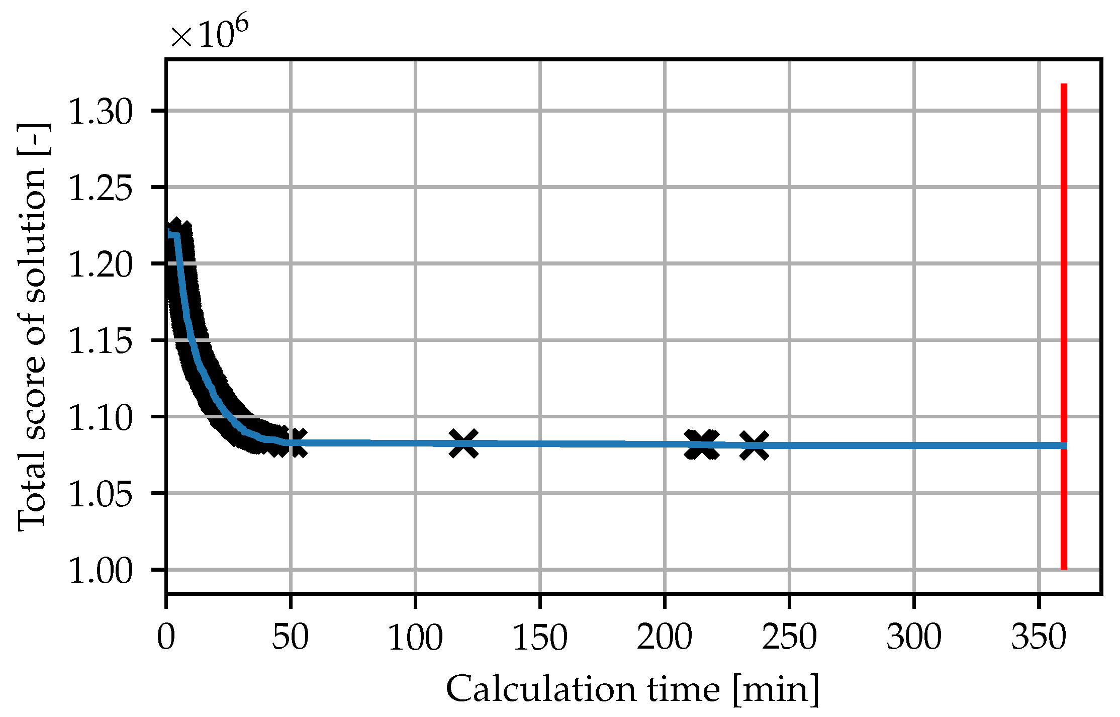
6.1. Fleet Sizing Based on Flight Scheduling
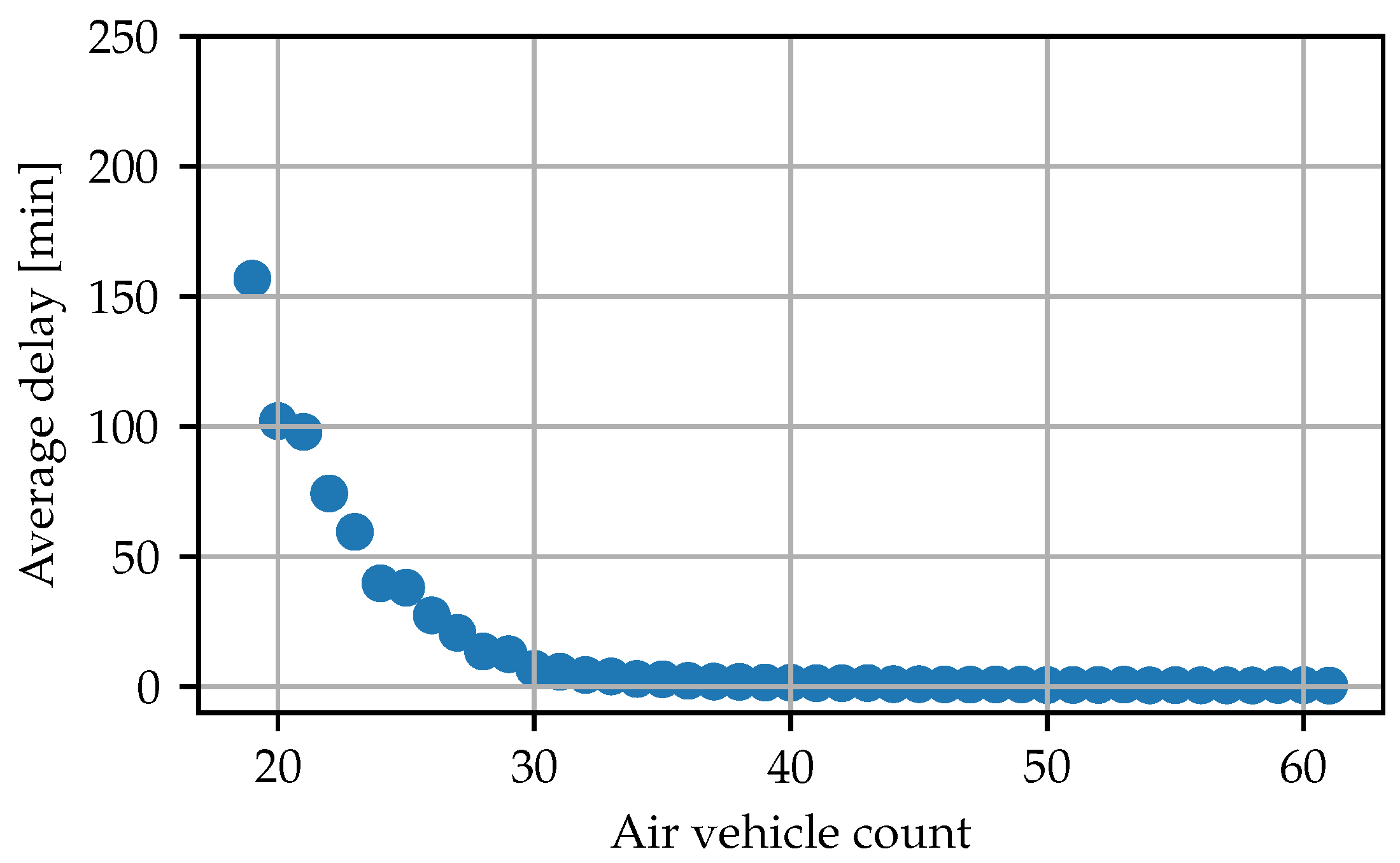
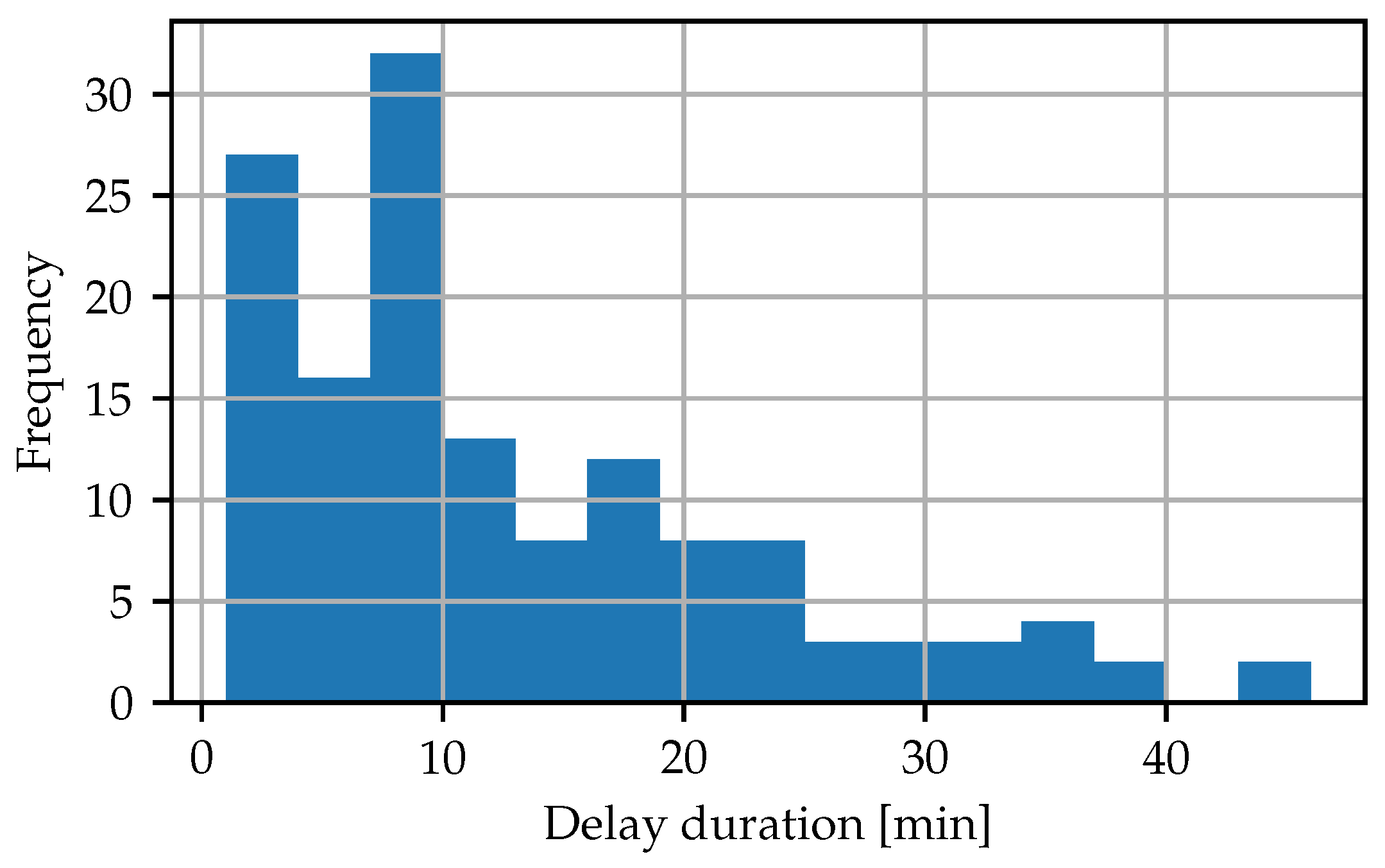
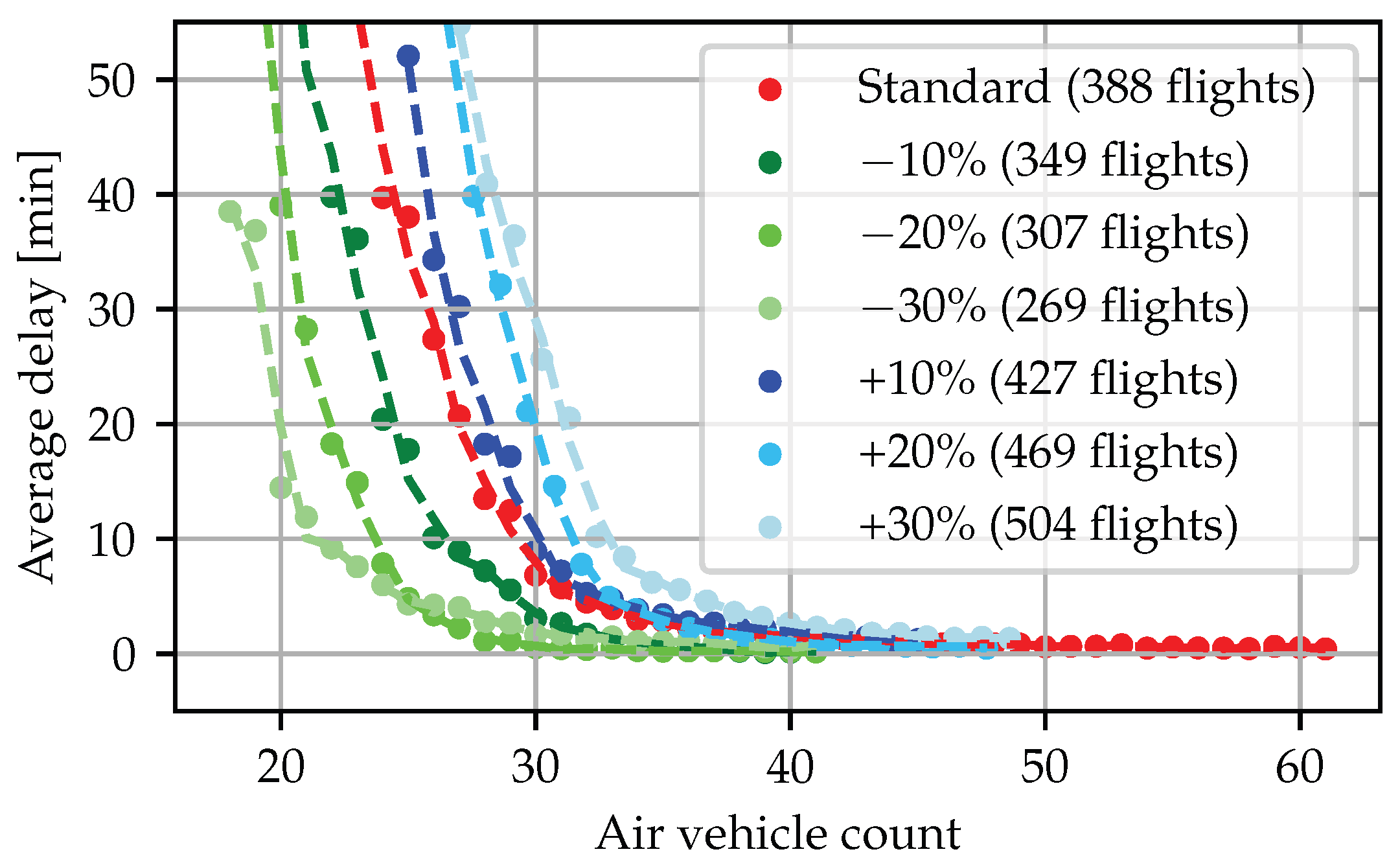
6.1.1. Average Delay in the Standard Demand Scenario
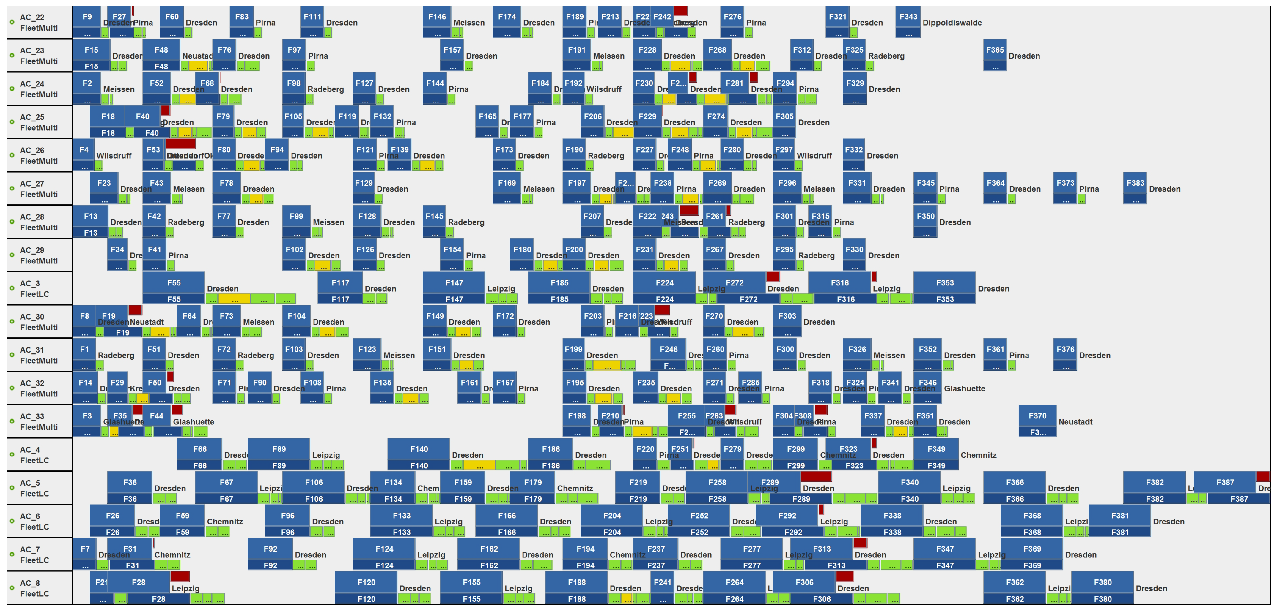
6.1.2. Best Solution Characteristics (32 Air Taxi)
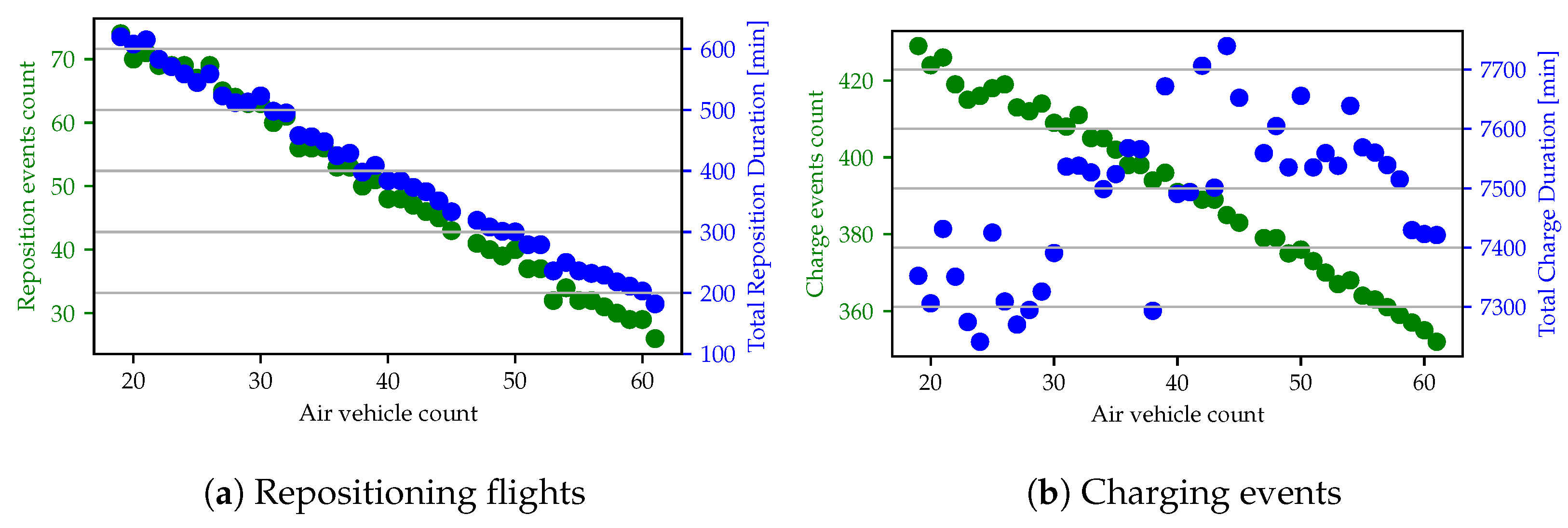
6.1.3. Effect of Repositioning Flights on Efficiency
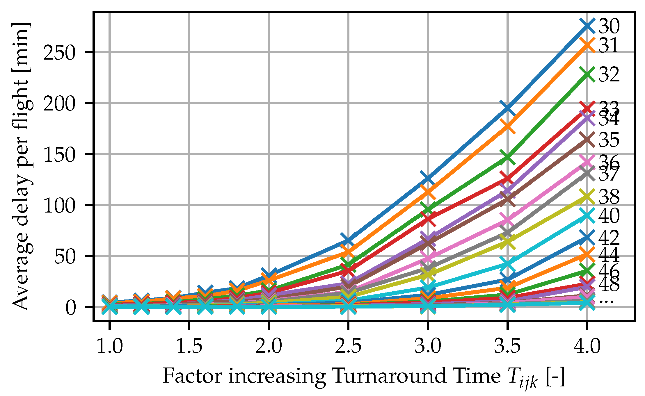
6.2. Parameter Study; Standard Demand Scenario, 32 Air Taxis
6.2.1. Turnaround Time
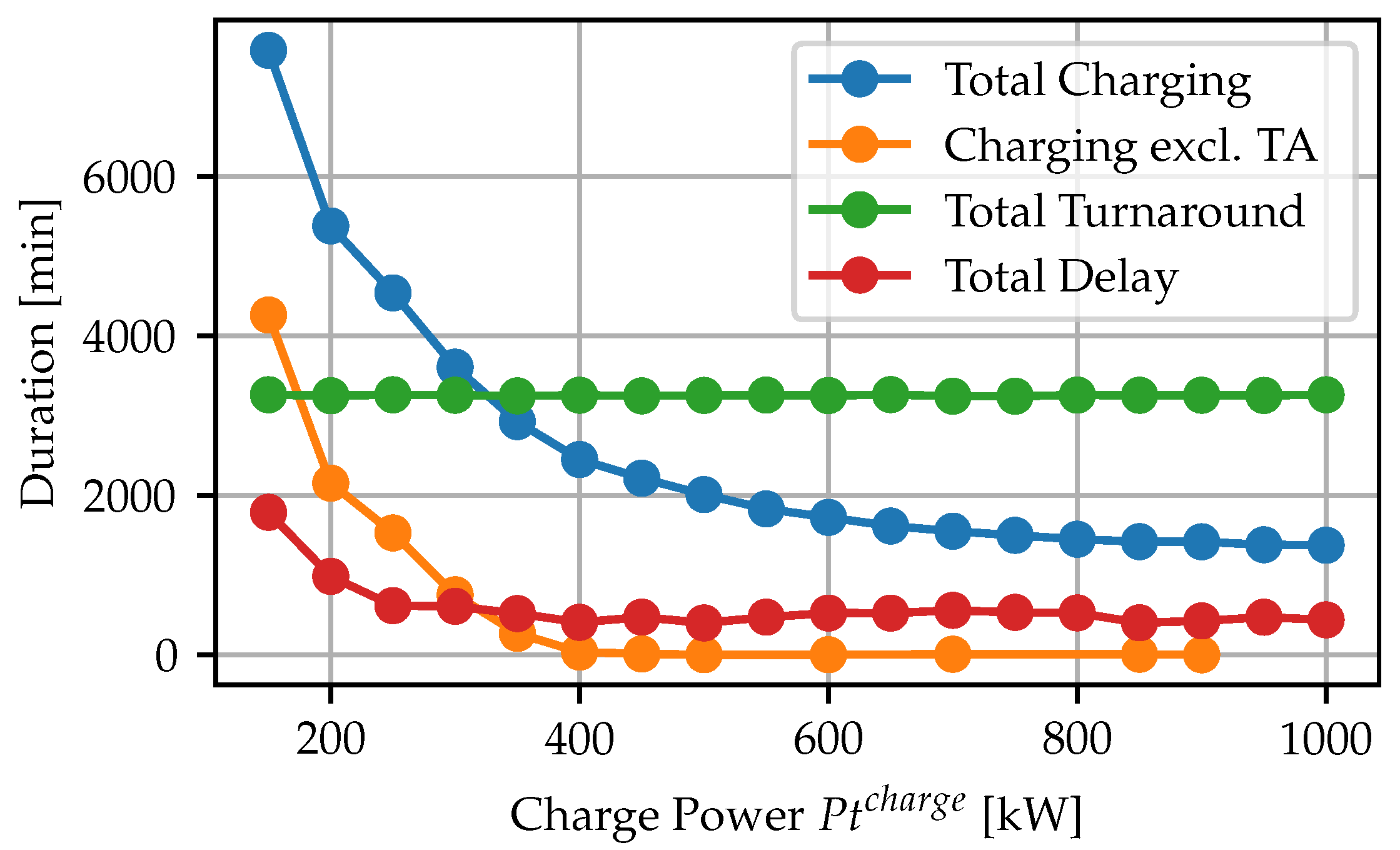
6.2.2. Charging Performance
6.3. Changes in Forecasted Demand
7. Discussion
7.1. Practical and Theoretical Implications
7.2. Conclusions and Future Research
Author Contributions
Funding
Institutional Review Board Statement
Informed Consent Statement
Data Availability Statement
Conflicts of Interest
Appendix A
Appendix A.1

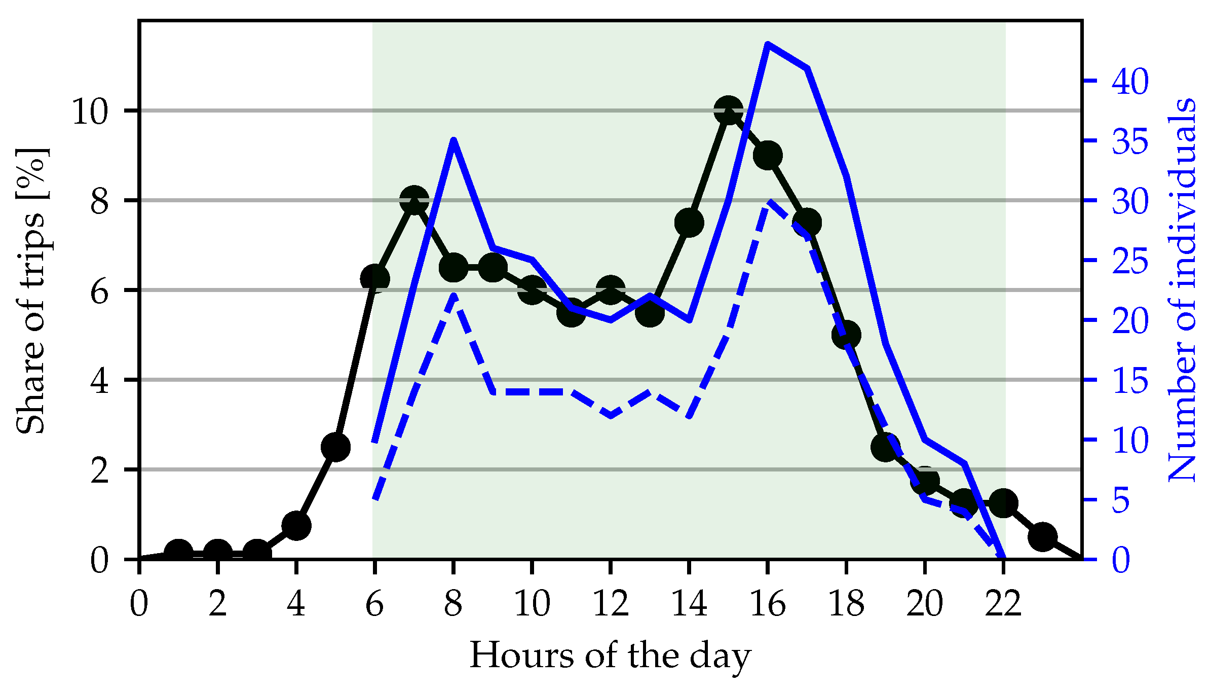
| Day Hour | Relative Share of Trips | |
|---|---|---|
| 00:00–00:59 a.m. | 0 | |
| 01:00–01:59 a.m. | 0.001 | |
| 02:00–02:59 a.m. | 0.001 | |
| 03:00–03:59 a.m. | 0.001 | Night flight restriction |
| 04:00–04:59 a.m. | 0.0075 | |
| 05:00–05:59 a.m. | 0.025 | |
| 06:00–06:59 a.m. | 0.0625 | |
| 07:00–07:59 a.m. | 0.08 | |
| 08:00–08:59 a.m. | 0.065 | |
| 09:00–09:59 a.m. | 0.065 | |
| 10:00–10:59 a.m. | 0.06 | |
| 11:00–11:59 a.m. | 0.0535 | |
| 12:00–12:59 p.m. | 0.06 | |
| 01:00–01:59 p.m. | 0.0535 | |
| 02:00–02:59 p.m. | 0.075 | Operation time |
| 03:00–03:59 p.m. | 0.01 | (green area in Figure 5) |
| 04:00–04:59 p.m. | 0.09 | |
| 05:00–05:59 p.m. | 0.075 | |
| 06:00–06:59 p.m. | 0.05 | |
| 07:00–07:59 p.m. | 0.025 | |
| 08:00–08:59 p.m. | 0.0175 | |
| 09:00–09:59 p.m. | 0.015 | |
| 10:00–10:59 p.m. | 0.015 | Night flight restriction |
| 11:00–11:59 p.m. | 0.005 | |
| Total | 1.0000 |
| Segment s | Vectored Thrust | Lift and Cruise | Multicopter |
|---|---|---|---|
| Hovertaxi | 6.04 | 3.22 | 0.45 |
| Vertical take-off and Transition (30 s) | 15.87 | 9.38 | 0.74 |
| Vertical take-off and Transition (45 s) | 19.23 | 11.22 | 1.10 |
| Vertical take-off and Transition (60 s) | 22.59 | 13.06 | 1.47 |
| Vertical take-off and Transition (75 s) | 25.95 | 14.90 | 1.84 |
| Vertical take-off and Transition (90 s) | 29.31 | 16.74 | 2.21 |
| Transition and vertical landing (30 s) | 14.59 | 8.51 | 0.28 |
| Transition and vertical landing (30 s) | 17.30 | 9.91 | 0.42 |
| Transition and vertical landing (30 s) | 20.02 | 11.31 | 0.55 |
| Transition and vertical landing (30 s) | 22.74 | 12.72 | 0.69 |
| Transition and vertical landing (30 s) | 25.46 | 14.12 | 0.83 |
| Groundtaxi | 0.10 | 0.06 | 0.07 |
| Destination | Distance GCD | Cruise Distance | Cruise Duration | Total Horizontal Duration | Energy Consumption |
|---|---|---|---|---|---|
| [m] | [m] | [s] | [s] | [kWh] | |
| Vectored Thrust | |||||
| Kreischa | 11,900 | 6403 | 89 | 242 | 8.15 |
| Moritzburg | 12,600 | 7103 | 99 | 251 | 8.48 |
| Wilsdruff | 13,900 | 8403 | 117 | 269 | 9.09 |
| Radeberg | 14,800 | 9303 | 129 | 282 | 9.51 |
| Ottendorf-Okr. | 16,500 | 11,003 | 153 | 306 | 10.30 |
| Pirna | 17,400 | 11,903 | 165 | 318 | 10.72 |
| Dippoldisw. | 17,900 | 12,403 | 172 | 325 | 10.96 |
| Meißen | 22,300 | 16,803 | 233 | 386 | 13.02 |
| Glashütte | 22,400 | 16,903 | 235 | 387 | 13.07 |
| Altenberg | 31,800 | 26,303 | 365 | 518 | 17.47 |
| Neustadt/S. | 33,500 | 28,003 | 389 | 542 | 18.26 |
| Chemnitz | 62,100 | 56,603 | 786 | 939 | 31.66 |
| Leipzig | 99,900 | 94,403 | 1311 | 1464 | 49.39 |
| Lift and Cruise | |||||
| Kreischa | 11,900 | 9781 | 245 | 350 | 6.72 |
| Moritzburg | 12,600 | 10,481 | 262 | 368 | 7.05 |
| Wilsdruff | 13,900 | 11,781 | 295 | 400 | 7.67 |
| Radeberg | 14,800 | 12,681 | 317 | 423 | 8.11 |
| Ottendorf-Okr. | 16,500 | 14,381 | 360 | 465 | 8.92 |
| Pirna | 17,400 | 15,281 | 382 | 488 | 9.35 |
| Dippoldisw. | 17,900 | 15,781 | 395 | 500 | 9.59 |
| Meißen | 22,300 | 20,181 | 505 | 610 | 11.70 |
| Glashütte | 22,400 | 20,281 | 507 | 613 | 11.75 |
| Altenberg | 31,800 | 29,681 | 742 | 848 | 16.25 |
| Neustadt/S. | 33,500 | 31,381 | 785 | 980 | 17.07 |
| Chemnitz | 62,100 | 59,981 | 1500 | 1605 | 30.77 |
| Leipzig | 99,900 | 97,781 | 2445 | 2550 | 48.88 |
| Multicopter | |||||
| Kreischa | 11,900 | 10,918 | 455 | 537 | 13.16 |
| Moritzburg | 12,600 | 11,618 | 484 | 566 | 13.88 |
| Wilsdruff | 13,900 | 12,918 | 538 | 620 | 15.21 |
| Radeberg | 14,800 | 13,818 | 576 | 658 | 16.13 |
| Ottendorf-Okr. | 16,500 | 15,518 | 647 | 728 | 17.86 |
| Pirna | 17,400 | 16,418 | 684 | 766 | 18.78 |
| Dippoldisw. | 17,900 | 16,918 | 705 | 787 | 19.29 |
| Meißen | 22,300 | 21,318 | 888 | 970 | 23.79 |
| Glashütte | 22,400 | 21,418 | 892 | 974 | 23.89 |
| Altenberg | 31,800 | 30,818 | 1284 | 1366 | 33.50 |
| Neustadt/S. | 33,500 | 32,518 | 1355 | 1437 | 35.24 |
| Chemnitz | 62,100 | 561,118 | 2547 | 2628 | 64.46 |
| Leipzig | 99,900 | 98,918 | 4122 | 4203 | 103.09 |
References
- UAM Initiative Cities Community (UIC2). Manifesto on the Multilevel Governance of the Urban Sky. 2020. Available online: https://civitas.eu/sites/default/files/UIC2%20Manifesto%20-%20Multilevel%20Governance%20of%20the%20Urban%20Sky_wtih%20supporting%20cities_15Sep2022.pdf (accessed on 25 July 2023).
- European Commission (EC). Smart Cities. 2020. Available online: https://commission.europa.eu/eu-regional-and-urban-development/topics/cities-and-urban-development/city-initiatives/smart-cities_en (accessed on 10 January 2024).
- Agouridas, V.; Biermann, F.; Czaya, A.; Richter, D.; Stemmler, J.; Stęchły, J.; Witkowska-Konieczny, A.; Metropolia, G.; Kumar, R.; Metropole, T.; et al. Urban Air Mobility and Sustainable Urban Mobility Planning—Practioner Briefing. 12 2021. Available online: https://doi.org/10.6084/m9.figshare.19314005.v1 (accessed on 10 January 2024).
- Fraske, T. Change Agency and Path Creation toward Future Transport Systems: A Case Study of the Emerging Urban Air Mobility in Germany. 2022. Available online: http://dx.doi.org/10.13140/RG.2.2.27722.24000 (accessed on 11 January 2024).
- Brühl, R.; Fricke, H.; Tober, L.A.; Dexl, F.; Markmiller, J.; Walla, N.; Mutz, C.; Erfurt, R.; Fraske, T.; Medeiros, R.M.; et al. SmartFly—Concept for the Intelligent Integration and Economic Use of Air Taxis in Saxony. 2022. Available online: https://doi.org/10.13140/RG.2.2.24570.98245 (accessed on 11 January 2024).
- Vallée, D.; Engel, B.; Vogt, W. (Eds.) Stadtverkehrsplanung Band 1; Springer: Berlin/Heidelberg, Germany, 2021. [Google Scholar] [CrossRef]
- Teodorović, D.; Janić, M. Transportation Engineering: Theory, Practice, and Modeling, 2nd ed.; Butterworth-Heinemann: Cambridge, UK, 2022. [Google Scholar]
- Gerike, R.; Hubrich, S.; Ließke, F.; Wittig, S.; Wittwer, R. Sonderauswertung “Mobilität in Städten—SrV 2018”: Oberzentren 500.000 und mehr EW, Topografie Flach (“Mobility in Cities—SrV”: Tables for High-Order Cities of 500,000 and More Inhabitants and with Flat Topography for the Year 2018). 2020. Available online: https://www.researchgate.net/publication/340273317_Sonderauswertung_Mobilitat_in_Stadten_-_SrV_2018_Oberzentren_500000_und_mehr_EW_Topografie_flach_Mobility_in_Cities_-_SrV_Tables_for_high-order_cities_of_500000_and_more_inhabitants_and_with_flat_topo (accessed on 11 January 2024).
- Nobis, C.; Kuhnimhof, T.; Follmer, R.; Bäumer, M. Mobilität in Deutschland—MiD: Zeitreihenbericht 2002–2008–2017. 2019. Available online: https://bmdv.bund.de/SharedDocs/DE/Anlage/G/mid-zeitreihenbericht-2002-2008-2017.pdf?__blob=publicationFile (accessed on 10 January 2024).
- Kumar, S.P.; Vinay, M.; Joshi, G.J. Transportation Planning: Principles, Practises and Policies, 2nd ed.; PHI Learning Private Limited: Delhi, India, 2017. [Google Scholar]
- Ben-Akiva, M.E.; Lerman, S.R. Discrete Choice Analysis: Theory and Application to Travel Demand; Number 9 in MIT Press Series in Transportation Studies; MIT Press: Cambridge, MA, USA, 1985. [Google Scholar]
- Golob, T.F.; Beckmann, M.J.; Zahavi, Y. A utility-theory travel demand model incorporating travel budgets. Transp. Res. Part Methodol. 1981, 15, 375–389. [Google Scholar] [CrossRef]
- Sun, X.; Wandelt, S.; Husemann, M.; Stumpf, E. Operational Considerations regarding On-Demand Air Mobility: A Literature Review and Research Challenges. J. Adv. Transp. 2021, 2021, 3591034. [Google Scholar] [CrossRef]
- Balac, M. The market potential of Urban Air Mobility in the USA: Analysis based on open-data. In Proceedings of the 2021 IEEE International Intelligent Transportation Systems Conference (ITSC), Indianapolis, IN, USA, 19–22 September 2021; pp. 1419–1424. [Google Scholar] [CrossRef]
- Justin, C.Y.; Payan, A.P.; Mavris, D. Demand modeling and operations optimization for advanced regional air mobility. In Proceedings of the AIAA AVIATION 2021 FORUM, Virtual Event, 2–6 August 2021; p. 3179. [Google Scholar] [CrossRef]
- Rajendran, S.; Srinivas, S.; Grimshaw, T. Predicting demand for air taxi urban aviation services using machine learning algorithms. J. Air Transp. Manag. 2021, 92, 102043. [Google Scholar] [CrossRef]
- Wu, Z.; Zhang, Y. Integrated Network Design and Demand Forecast for On-Demand Urban Air Mobility. Engineering 2021, 7, 473–487. [Google Scholar] [CrossRef]
- Bulusu, V.; Onat, E.B.; Sengupta, R.; Yedavalli, P.; Macfarlane, J. A traffic demand analysis method for urban air mobility. IEEE Trans. Intell. Transp. Syst. 2021, 22, 6039–6047. [Google Scholar] [CrossRef]
- Yedavalli, P.S.; Onat, E.; Peng, X.; Sengupta, R.; Waddell, P.; Bulusu, V.; Xue, M. Assessing the Value of Urban Air Mobility through Metropolitan-Scale Microsimulation: A Case Study of the San Francisco Bay Area. In Proceedings of the AIAA AVIATION 2021 FORUM, Virtual Event, 2–6 August 2021; p. 2338. [Google Scholar] [CrossRef]
- Rothfeld, R.; Fu, M.; Balać, M.; Antoniou, C. Potential urban air mobility travel time savings: An exploratory analysis of Munich, Paris, and San Francisco. Sustainability 2021, 13, 2217. [Google Scholar] [CrossRef]
- Park, B.T.; Kim, H.; Kim, S.H. Vertiport Performance Analysis for On-Demand Urban Air Mobility Operation in Seoul Metropolitan Area. Int. J. Aeronaut. Space Sci. 2022, 23, 1065–1078. [Google Scholar] [CrossRef]
- Jeong, J.; So, M.; Hwang, H.Y. Selection of Vertiports Using K-Means Algorithm and Noise Analyses for Urban Air Mobility (UAM) in the Seoul Metropolitan Area. Appl. Sci. 2021, 11, 5729. [Google Scholar] [CrossRef]
- Peksa, M.; Bogenberger, K. Estimating UAM Network Load with Traffic Data for Munich. In Proceedings of the 2020 AIAA/IEEE 39th Digital Avionics Systems Conference (DASC), San Antonio, TX, USA, 11–15 October 2020; pp. 1–7. [Google Scholar] [CrossRef]
- Fu, M.; Straubinger, A.; Schaumeier, J. Scenario-based Demand Assessment of Urban Air Mobility in the Greater Munich Area. J. Air Transp. 2022, 30, 125–136. [Google Scholar] [CrossRef]
- Balac, M.; Rothfeld, R.L.; Hörl, S. The prospects of on-demand urban air mobility in Zurich, Switzerland. In Proceedings of the 2019 IEEE Intelligent Transportation Systems Conference (ITSC), Auckland, New Zealand, 27–30 October 2019; pp. 906–913. [Google Scholar] [CrossRef]
- Finkeldei, W.; Feldhoff, E.; Roque, G.S. Flughafen Köln/Bonn Flugtaxi Infrastruktur: Machbarkeitsstudie; Flughafen Köln/Bonn GmbH: Cologne, Germany, 2020. (In Germany) [Google Scholar]
- Götz, K.; Deffner, J.; Klinger, T. Mobilitätsstile und Mobilitätskulturen–Erklärungspotentiale, Rezeption und Kritik. In Handbuch Verkehrspolitik; Springer: Wiesbaden, Germany, 2016; pp. 781–804. [Google Scholar] [CrossRef]
- Batty, P.; Palacin, R.; González-Gil, A. Challenges and opportunities in developing urban modal shift. Travel Behav. Soc. 2015, 2, 109–123. [Google Scholar] [CrossRef]
- Riza, L.; Bruehl, R.; Fricke, H.; Planing, P. Will air taxis extend public transportation? A scenario-based approach on user acceptance in different urban settings. Transp. Res. Interdiscip. Perspect. 2024, 23, 101001. [Google Scholar] [CrossRef]
- Straubinger, A.; Rothfeld, R.; Shamiyeh, M.; Büchter, K.D.; Kaiser, J.; Plötner, K.O. An overview of current research and developments in urban air mobility–Setting the scene for UAM introduction. J. Air Transp. Manag. 2020, 87, 101852. [Google Scholar] [CrossRef]
- Brühl, R.; Fricke, H.; Schultz, M. Air taxi flight performance modeling and application. In Proceedings of the ATM Seminar, Virtual, 20–24 September 2021. [Google Scholar]
- Lee, B.S.; Yun, J.Y.; Hwang, H.Y. Flight Range and Time Analysis for Classification of eVTOL PAV. J. Adv. Navig. Technol. 2020, 24, 73–84. [Google Scholar] [CrossRef]
- Bacchini, A.; Cestino, E. Electric VTOL configurations comparison. Aerospace 2019, 6, 26. [Google Scholar] [CrossRef]
- Rajendran, S.; Zack, J. Insights on strategic air taxi network infrastructure locations using an iterative constrained clustering approach. Transp. Res. Part E Logist. Transp. Rev. 2019, 128, 470–505. [Google Scholar] [CrossRef]
- The Vertical Flight Society. eVTOL Aircraft Directory. 2022. Available online: https://evtol.news/aircraft (accessed on 10 January 2024).
- Datta, A.; Elbers, S.; Wakayama, S.; Alonso, J.; Botero, E.; Carter, C.; Martins, F. Commercial Intra-City On-Demand Electric-VTOL Status of Technology. AHS/NARI Transformative Vertical Flight Working Group-2; 2018. Available online: https://vtol.org/files/dmfile/TVF.WG2.YR2017draft.pdf (accessed on 11 January 2024).
- Miao, Y.; Hynan, P.; von Jouanne, A.; Yokochi, A. Current Li-Ion Battery Technologies in Electric Vehicles and Opportunities for Advancements. Energies 2019, 12, 1074. [Google Scholar] [CrossRef]
- Cadex Electronics. BU-216: Summary Table of Lithium-Based Batteries. 2020. Available online: https://batteryuniversity.com/article/bu-216-summary-table-of-lithium-based-batteries (accessed on 10 January 2024).
- International Civil Aviation Organisation (ICAO). Procedures for Air Navigation Services (PANS) Aircraft Operations (OPS). 2018. Available online: https://ffac.ch/wp-content/uploads/2020/11/ICAO-Doc-8168-Volume-III-Aircraft-Operating-Procedures-.pdf (accessed on 11 January 2024).
- Shamiyeh, M.; Rothfeld, R.; Hornung, M. A performance benchmark of recent personal air vehicle concepts for urban air mobility. In Proceedings of the 31st Congress of the International Council of the Aeronautical Sciences, Belo Horizonte, Brazil, 9–14 September 2018. [Google Scholar]
- UBER Elevate. Uber Air Vehicle Requirements and Missions. 2018. Available online: https://s3.amazonaws.com/uber-static/elevate/Summary+Mission+and+Requirements.pdf (accessed on 11 January 2024).
- Brühl, R.; Fricke, H. Assessment of minimum ground time for air taxis based on turnaround critical path modeling. In Proceedings of the 10th Edition of the International Conference on Research in Air Transportation (ICRAT), Tampa, FL, USA, 19–23 June 2022. [Google Scholar]
- Beamon, B.M.; Chen, V.C.P. Performability-based fleet sizing in a material handling system. Int. J. Adv. Manuf. Technol. 1998, 14, 441–449. [Google Scholar] [CrossRef]
- Imen, L.; Wassim, M.; Mounir, E.; Hedi, C. Improvement opportunities of a Simulation/Expert System Approach for Manufacturing System Sizing: A review and proposal. Adv. Sci. Technol. Eng. Syst. J. 2019, 4, 213–223. [Google Scholar] [CrossRef]
- Ehlers, S.; Pache, H.; von Bock und Polach, F.; Johnsen, T. A Fleet Efficiency Factor for fleet size and mix problems using particle swarm optimisation. Ship Technol. Res. 2019, 66, 106–116. [Google Scholar] [CrossRef]
- Cheng, L.; Wang, K.; De Vos, J.; Huang, J.; Witlox, F. Exploring non-linear built environment effects on the integration of free-floating bike-share and urban rail transport: A quantile regression approach. Transp. Res. Part A Policy Pract. 2022, 162, 175–187. [Google Scholar] [CrossRef]
- Guidon, S.; Reck, D.J.; Axhausen, K. Expanding a (n)(electric) bicycle-sharing system to a new city: Prediction of demand with spatial regression and random forests. J. Transp. Geogr. 2020, 84, 102692. [Google Scholar] [CrossRef]
- Kania, M.; Assmann, T. Data-Driven Approach for Defining Demand Scenarios for Shared Autonomous Cargo-Bike Fleets. In Smart Energy for Smart Transport: Proceedings of the 6th Conference on Sustainable Urban Mobility, CSUM2022, Skiathos Island, Greece, 31 August–2 September 2022; Springer: Berlin/Heidelberg, Germany, 2023; pp. 1374–1405. [Google Scholar] [CrossRef]
- Hua, M.; Chen, X.; Chen, J.; Jiang, Y. Minimizing fleet size and improving vehicle allocation of shared mobility under future uncertainty: A case study of bike sharing. J. Clean. Prod. 2022, 370, 133434. [Google Scholar] [CrossRef]
- Wittmann, M.; Neuner, L.; Lienkamp, M. A Predictive Fleet Management Strategy for On-Demand Mobility Services: A Case Study in Munich. Electronics 2020, 9, 1021. [Google Scholar] [CrossRef]
- Ye, X.; Li, M.; Yang, Z.; Yan, X.; Chen, J. A dynamic adjustment model of cruising taxicab fleet size combined the operating and flied survey data. Sustainability 2020, 12, 2776. [Google Scholar] [CrossRef]
- Ko, S.; Lautala, P.; Zhang, K. Data-Driven Study on the Sustainable Log Movements: Impact of Rail Car Fleet Size on Freight Storage and Car Idling. Sustainability 2020, 12, 4563. [Google Scholar] [CrossRef]
- Csereklyei, Z.; Stern, D.I. Flying more efficiently: Joint impacts of fuel prices, capital costs and fleet size on airline fleet fuel economy. Ecol. Econ. 2020, 175, 106714. [Google Scholar] [CrossRef]
- Müller, C.; Kieckhäfer, K.; Spengler, T.S. The influence of emission thresholds and retrofit options on airline fleet planning: An optimization approach. Energy Policy 2018, 112, 242–257. [Google Scholar] [CrossRef]
- Mohri, S.S.; Nasrollahi, M.; Pirayesh, A.; Mohammadi, M. An integrated global airline hub network design with fleet planning. Comput. Ind. Eng. 2022, 164, 107883. [Google Scholar] [CrossRef]
- Liu, M.; Ding, Y.; Sun, L.; Zhang, R.; Dong, Y.; Zhao, Z.; Wang, Y.; Liu, C. Green Airline-Fleet Assignment with Uncertain Passenger Demand and Fuel Price. Sustainability 2023, 15, 899. [Google Scholar] [CrossRef]
- Agrawal, P.; Pravinvongvuth, S. Estimation of Travel Demand for Bangkok; Chiang Mai Hyperloop Using Traveler Surveys. Sustainability 2021, 13, 14037. [Google Scholar] [CrossRef]
- Sha, M.; Srinivasan, R. Fleet sizing in chemical supply chains using agent-based simulation. Comput. Chem. Eng. 2016, 84, 180–198. [Google Scholar] [CrossRef]
- Samchuk, G.; Kopytkov, D.; Rossolov, A. Freight Fleet Management Problem: Evaluation of a Truck Utilization Rate Based on Agent Modeling. Commun.-Sci. Lett. Univ. Zilina 2022, 24, D46–D58. [Google Scholar] [CrossRef]
- Valmiki, P.; Reddy, A.S.; Panchakarla, G.; Kumar, K.; Purohit, R.; Suhane, A. A study on simulation methods for AGV fleet size estimation in a flexible manufacturing system. Mater. Today Proc. 2018, 5, 3994–3999. [Google Scholar] [CrossRef]
- Saprykin, A.; Chokani, N.; Abhari, R.S. Impacts of downscaled inputs on the predicted performance of taxi fleets in agent-based scenarios including Mobility-as-a-Service. Procedia Comput. Sci. 2022, 201, 574–580. [Google Scholar] [CrossRef]
- Rajendran, S.; Shulman, J. Study of emerging air taxi network operation using discrete-event systems simulation approach. J. Air Transp. Manag. 2020, 87, 101857. [Google Scholar] [CrossRef]
- Papier, F.; Thonemann, U.W. Queuing Models for Sizing and Structuring Rental Fleets. Transp. Sci. 2008, 42, 302–317. [Google Scholar] [CrossRef]
- Fanti, M.P.; Mangini, A.M.; Pedroncelli, G.; Ukovich, W. Fleet sizing for electric car sharing system via closed queueing networks. In Proceedings of the 2014 IEEE International Conference on Systems, Man, and Cybernetics (SMC), San Diego, CA, USA, 5–8 October 2014; pp. 1324–1329. [Google Scholar] [CrossRef]
- Amjath, M.; Kerbache, L.; Smith, J.M.; Elomri, A. Fleet sizing of trucks for an inter-facility material handling system using closed queueing networks. Oper. Res. Perspect. 2022, 9, 100245. [Google Scholar] [CrossRef]
- Golden, B.; Assad, A.; Levy, L.; Gheysens, F. The fleet size and mix vehicle routing problem. Comput. Oper. Res. 1984, 11, 49–66. [Google Scholar] [CrossRef]
- Vis, I.F.; de Koster, R.M.B.; Savelsbergh, M.W. Minimum vehicle fleet size under time-window constraints at a container terminal. Transp. Sci. 2005, 39, 249–260. [Google Scholar] [CrossRef]
- Li, Z.; Tao, F. On determining optimal fleet size and vehicle transfer policy for a car rental company. Comput. Oper. Res. 2010, 37, 341–350. [Google Scholar] [CrossRef]
- Repoussis, P.; Tarantilis, C. Solving the Fleet Size and Mix Vehicle Routing Problem with Time Windows via Adaptive Memory Programming. Transp. Res. Part C Emerg. Technol. 2010, 18, 695–712. [Google Scholar] [CrossRef]
- Koç, Ç.; Bektaş, T.; Jabali, O.; Laporte, G. The fleet size and mix location-routing problem with time windows: Formulations and a heuristic algorithm. Eur. J. Oper. Res. 2016, 248, 33–51. [Google Scholar] [CrossRef]
- Jara-Díaz, S.; Fielbaum, A.; Gschwender, A. Optimal fleet size, frequencies and vehicle capacities considering peak and off-peak periods in public transport. Transp. Res. Part A Policy Pract. 2017, 106, 65–74. [Google Scholar] [CrossRef]
- Dresdner Verkehrsbetriebe, A.G.; Landeshauptstadt Dresden, V. Traditionen, Trips & Trends—Mobilität in Dresden und Umland unter der Lupe - Ergebnisse aus der Verkehrserhebung SrV [German], 2018. Available online: https://www.dresden.de/media/pdf/stadtplanung/verkehr/SrV_2018_Broschuere.pdf (accessed on 11 January 2024).
- Gesellschaft für Luftverkehrsforschung (GfL). Bereitstellung Lokaler Mobilitätsparameter und Mobilitätseigenschaften für Lufttaxis auf Basis Bundesweiter Daten Gemäß den Befragungen “Mobilität in Deutschland” und “Verkehr in Städten” [German]; Gesellschaft für Luftverkehrsforschung (GfL): Dresden, Germany, 2022. [Google Scholar]
- Brühl, R.; Fricke, H. Locating air taxi infrastructure in regional areas—The Saxony use case. In Proceedings of the Deutscher Luft-und Raumfahrtkongress (DLRK) 2022, Dresden, Germany, 29 September 2022. [Google Scholar]
- Krueger, R.; Rashidi, T.H.; Rose, J.M. Preferences for shared autonomous vehicles. Transp. Res. Part C Emerg. Technol. 2016, 69, 343–355. [Google Scholar] [CrossRef]
- Fu, M.; Rothfeld, R.; Antoniou, C. Exploring preferences for transportation modes in an urban air mobility environment: Munich case study. Transp. Res. Rec. 2019, 2673, 427–442. [Google Scholar] [CrossRef]
- Thompson, M. Panel: Perspectives on prospective markets. In Proceedings of the 5th Annual AHS Transformative VTOL Workshop, San Francisco, CA, USA, 18–19 January 2018; pp. 18–19. [Google Scholar]
- Shaheen, S.; Cohen, A.; Farrar, E. The Potential Societal Barriers of Urban Air Mobility (UAM). 2018. Available online: https://doi.org/10.7922/G28C9TFR (accessed on 11 January 2024).
- Statistisches Landesamt des Freistaates Sachsen. Bevölkerungsstand, Einwohnerzahlen. 2021. Available online: https://www.statistik.sachsen.de/\html/bevoelkerungsstand-einwohner.html (accessed on 10 January 2024).
- Statistische Ämter der Länder. Pendleratlas Deutschland. 2023. Available online: https://pendleratlas.statistikportal.de/ (accessed on 10 January 2024).
- Johnson, W. Helicopter Theory; Princeton University Press: Princeton, NJ, USA, 1980. [Google Scholar]
- van der Wall, B.G. Grundlagen der Hubschrauber-Aerodynamik (German); Springer: Berlin/Heidelberg, Germany, 2020. [Google Scholar]
- Kamal, A.M.; Ramirez-Serrano, A. Design methodology for hybrid (VTOL + Fixed Wing) unmanned aerial vehicles. Aeronaut. Aerosp. Open Access J. 2018, 2, 165–176. [Google Scholar] [CrossRef]
- Patterson, M.; Antcliff, K.; Kohlman, L. A proposed Approach to Studying Urban Air Mobility Missions including an Initial Exploration of Mission Requirements. In Proceedings of the AHS International 74th Annual Forum & Technology Display, Phoenix, AZ, USA, 15–17 May 2018. [Google Scholar]
- Rosenow, J.; Zeh, T.; Lindner, M.; Förster, S.; Fricke, H.; Caraud, A. Multiple Aircraft in a multi-criteria Trajectory Optimization. In Proceedings of the Fifteenth USA/Europe Air Traffic Management Research and Development Seminar (ATM2023), Savannah, GA, USA, 5–9 June 2023. [Google Scholar]
- Sun, J.; Ellerbroek, J.; Hoekstra, J. Modeling aircraft performance parameters with open ADS-B data. In Proceedings of the 12th USA/Europe Air Traffic Management Research and Development Seminar, Seattle, WA, USA, 27–30 June 2017. [Google Scholar]
- Hepperle, M. Electric Flight—Potential and Limitations. In Proceedings of the AVT-209 Workshop on Energy Efficient Technologies and Concepts of Operation, Lisbon, Portugal, 22–24 October 2012. [Google Scholar]
- Evler, J.; Lindner, M.; Fricke, H.; Schultz, M. Integration of turnaround and aircraft recovery to mitigate delay propagation in airline networks. Comput. Oper. Res. 2022, 138, 105602. [Google Scholar] [CrossRef]
- Lindner, M.; Fricke, H. Performance Degradation based Aircraft Tail Assignment and Routing in Daily Airline Operations. In Proceedings of the Deutscher Luft- und Raumfahrtkongress DLRK 2022, Dresden, Germany, 27–29 September 2022. [Google Scholar]
- De Smet, G.; Open Source Contributors. OptaPlanner User Guide; Red Hat, Inc. or Third-Party Contributors, 2006; OptaPlanner is an Open Source Constraint Solver in Java. Available online: https://docs.optaplanner.org/latest/optaplanner-docs/html_single/index.html (accessed on 25 July 2023).
- De Neufville, R. Airport systems planning, design, and management. In Air Transport Management; Routledge: Abingdon, UK, 2020; pp. 79–96. [Google Scholar]
- Chen, L.; Wandelt, S.; Dai, W.; Sun, X. Scalable Vertiport Hub Location Selection for Air Taxi Operations in a Metropolitan Region. INFORMS J. Comput. 2022, 34, 834–856. [Google Scholar] [CrossRef]


| City | # Trips | Rel. Share [%] | GCD [km] |
|---|---|---|---|
| Pirna | 103 | 9.0 | 17.4 |
| Radeberg | 77 | 6.7 | 14.8 |
| Meißen | 46 | 4.0 | 22.3 |
| Glashütte | 46 | 4.0 | 22.4 |
| Wilsdruff | 38 | 3.3 | 13.9 |
| Ottendorf-Okrilla | 32 | 2.8 | 16.5 |
| Leipzig | 29 | 2.6 | 99.9 |
| Altenberg | 27 | 2.4 | 31.8 |
| Kreischa | 22 | 1.9 | 11.9 |
| Moritzburg | 22 | 1.9 | 12.6 |
| Dippoldiswalde | 20 | 1.8 | 17.9 |
| Neustadt in Sachsen | 18 | 1.6 | 33.5 |
| Chemnitz | 17 | 1.5 | 62.1 |
| Total | 497 | 43.5 | - |
| Bicycle | Car | Public Transport | Total |
|---|---|---|---|
| 0.43 | 3.24 | 1.08 | 4.75 |
| City | # Indv. | Car | Public Transport | Bicycle | AAM | ||||||
|---|---|---|---|---|---|---|---|---|---|---|---|
| rel. | abs. | AAM | rel. | abs. | AAM | rel. | abs. | AAM | Total | ||
| Pirna | 3481 | 0.73 | 2534 | 82.1 | 0.20 | 709 | 7.7 | 0.07 | 236 | 1.0 | 91 |
| Radeberg | 1266 | 0.70 | 887 | 28.8 | 0.25 | 312 | 3.4 | 0.05 | 65 | 0.3 | 32 |
| Meißen | 1141 | 0.63 | 719 | 23.3 | 0.30 | 347 | 3.7 | 0.07 | 74 | 0.3 | 27 |
| Glashütte | 268 | 0.93 | 250 | 8.1 | 0.07 | 17 | 0.2 | 0 | 0 | 0 | 8 |
| Wilsdruff | 480 | 0.84 | 404 | 13.1 | 0.16 | 75 | 0.8 | 0 | 0 | 0 | 14 |
| Ottend./Okr. | 280 | 0.94 | 262 | 8.5 | 0 | 0 | 0 | 0.06 | 17 | 0.1 | 9 |
| Leipzig | 15,309 | 0.48 | 7390 | 239.5 | 0.52 | 7918 | 85.5 | 0 | 0 | 0 | 325 |
| Altenberg | 190 | 1.00 | 190 | 6.2 | 0 | 0 | 0 | 0 | 0 | 0 | 6 |
| Kreischa | 87 | 0.91 | 79 | 2.6 | 0.09 | 7 | 0.1 | 0 | 0 | 0 | 3 |
| Moritzburg | 159 | 0.82 | 130 | 4.2 | 0.05 | 7 | 0.1 | 0.09 | 14 | 0.1 | 4 |
| Dippoldisw. | 254 | 0.80 | 203 | 6.6 | 0.20 | 50 | 0.6 | 0 | 0 | 0 | 7 |
| Neustadt/S | 189 | 0.89 | 168 | 5.5 | 0.11 | 21 | 0.2 | 0 | 0 | 0 | 6 |
| Chemnitz | 3695 | 0.59 | 2173 | 70.4 | 0.41 | 1521 | 16.4 | 0 | 0 | 0 | 87 |
| 619 | |||||||||||
| Parameter | Designation | Vect. Thrust | Lift and Cruise | Multicopter |
|---|---|---|---|---|
| Cruise speed | [m s−1] | 72 | 40 | 24 |
| Max. Take-Off Mass | [kg] | 2200 | 1600 | 900 |
| Payload | [kg] | 400 | 300 | 100 |
| Battery mass | [kg] | 730 | 530 | 300 |
| Battery mass ratio | [-] | 0.33 | ||
| Energy density | [W h kg−1] | 200 | ||
| Total energy | E [kW h] | 146 | 106 | 60 |
| Battery efficiency | [-] | 0.95 | ||
| Depth of discharge | [-] | 0.8 | ||
| Efficiency during hover | [-] | 0.70 | 0.75 | 0.8 |
| Efficiency during cruise | [-] | 0.8 | 0.7 | 0.6 |
| Efficiency during transition | [-] | 0.65 | 0.7 | - |
| Usable energy | [kW h] | 110.96 | 80.56 | 45.6 |
| Disc Loading | [ | 1354.98 | 832.70 | 59.03 |
| Air density | [ | 1.225 | ||
| Rotor rotation speed | [m s−1] | 23.52 | 18.44 | 4.91 |
| Rate of Climb | [m s−1] | 5 | ||
| Tilt angle | [°] | 82 | 90 | - |
| Total disc area | A [] | 8 | 9.4 | 74.8 |
| Wing surface | S [ | 11 | 11 | - |
| Solidity | [-] | 4.41 | 3.06 | - |
| Rotor tip speed | [m s−1] | 187 | ||
| Drag coefficient | [-] | 0.039 | 0.061 | 0.098 |
| Rotor drag coefficient | [-] | 0.0015 | ||
| Rotor diameter | [m] | 1.3 | 1.0 | 2.3 |
| Number of rotors | n [-] | 6 | 12 | 18 |
| Number of blades per rotor | N [-] | 5 | 2 | 2 |
| Lift-to-Drag ratio cruise | [-] | 16 | 13 | 4 |
| Taxi | Vertical Take-Off | Transition | Vertical Landing |
|---|---|---|---|
| 30 s | 30 s | 20 s | 30 s |
| Air Taxi | Cruise | Acceleration | Deceleration | ||
|---|---|---|---|---|---|
| Category | Speed [m s−1] | Distance [m] | Time [s] | Distance [m] | Time [s] |
| Vectored Thrust | 72 | 1177 | 33 | 4320 | 120 |
| Lift and Cruise | 40 | 519 | 26 | 1600 | 80 |
| Multicopter | 24 | 262 | 22 | 720 | 60 |
| Segment s | Vectored Thrust | Lift and Cruise | Multicopter |
|---|---|---|---|
| Hovertaxi | 725.07 | 385.82 | 54.17 |
| Vertical take-off | 806.23 | 441.67 | 88.38 |
| Transition | 1647.64 | 1025.46 | - |
| Cruise | 121.40 | 68.99 | 88.29 |
| Vertical landing | 651.07 | 337.03 | 33.20 |
| Groundtaxi | 12.14 | 6.90 | 8.83 |
| Destination | Vectored Thrust | Lift and Cruise | Multicopter | |||
|---|---|---|---|---|---|---|
| Total Energy Demand [kWh] | Total Duration [min] | Total Energy Demand [kWh] | Total Duration [min] | Total Energy Demand [kWh] | Total Duration [min] | |
| Kreischa | 44.8 | 6.7 | 27.9 | 8.5 | 14.7 | 10.9 |
| Moritzburg | 45.1 | 6.9 | 28.2 | 8.8 | 15.4 | 11.4 |
| Wilsdruff | 45.7 | 7.2 | 28.8 | 9.3 | 16.7 | 12.3 |
| Ottendorf-Okr. | 46.9 | 7.8 | 30.1 | 10.4 | 19.4 | 14.1 |
| Pirna | 47.3 | 8.0 | 30.5 | 10.8 | 20.3 | 14.8 |
| Dippoldisw. | 47.6 | 8.1 | 30.8 | 11.0 | 20.8 | 15.1 |
| Meißen | 49.6 | 9.1 | 32.9 | 12.8 | 25.3 | 18.2 |
| Glashütte | 49.7 | 9.1 | 32.9 | 12.9 | 25.4 | 18.2 |
| Altenberg | 54.1 | 11.3 | 37.4 | 16.8 | 35.0 | 24.8 |
| Neustadt/S. | 54.9 | 11.7 | 38.2 | 17.5 | 36.8 | 25.9 |
| Chemnitz | 68.3 | 18.3 | 51.9 | 29.4 | 66.0 | 45.8 |
| Leipzig | 86.0 | 27.1 | 70.0 | 45.2 | 104.6 | 72.1 |
| Vectored Thrust | Lift and Cruise | Multicopter | |
|---|---|---|---|
| Use Share | 10% | 50% | 40% |
| Avg. flight count per vehicle | |||
| Avg. vehicle utilization [h day−1] | |||
| Avg. recharge count per vehicle | |||
| Avg. recharge event (merged) [min] | |||
| Avg. duration of recharge [h vehicle−1] | |||
| Avg. reposition count per vehicle | 2 | ||
| Avg. duration of reposition [h vehicle−1] | |||
| Avg. distance per flight [km] | 90 | 84 | 19 |
| Avg. consumption per flight [kW h] | 84 | 64 | 21 |
| Avg. consumption per vehicle/day [kW h] | 811 | 681 | 302 |
Disclaimer/Publisher’s Note: The statements, opinions and data contained in all publications are solely those of the individual author(s) and contributor(s) and not of MDPI and/or the editor(s). MDPI and/or the editor(s) disclaim responsibility for any injury to people or property resulting from any ideas, methods, instructions or products referred to in the content. |
© 2024 by the authors. Licensee MDPI, Basel, Switzerland. This article is an open access article distributed under the terms and conditions of the Creative Commons Attribution (CC BY) license (https://creativecommons.org/licenses/by/4.0/).
Share and Cite
Lindner, M.; Brühl, R.; Berger, M.; Fricke, H. The Optimal Size of a Heterogeneous Air Taxi Fleet in Advanced Air Mobility: A Traffic Demand and Flight Scheduling Approach. Future Transp. 2024, 4, 174-214. https://doi.org/10.3390/futuretransp4010010
Lindner M, Brühl R, Berger M, Fricke H. The Optimal Size of a Heterogeneous Air Taxi Fleet in Advanced Air Mobility: A Traffic Demand and Flight Scheduling Approach. Future Transportation. 2024; 4(1):174-214. https://doi.org/10.3390/futuretransp4010010
Chicago/Turabian StyleLindner, Martin, Robert Brühl, Marco Berger, and Hartmut Fricke. 2024. "The Optimal Size of a Heterogeneous Air Taxi Fleet in Advanced Air Mobility: A Traffic Demand and Flight Scheduling Approach" Future Transportation 4, no. 1: 174-214. https://doi.org/10.3390/futuretransp4010010