1. Introduction
Shock waves originate from a sudden, substantial change in the state of the traffic flow [
1]. These are defined by an abrupt change in the flow-density conditions in the time–space domain. Efforts to classify shock waves matured to the point that they were commonly integrated into traffic engineering texts in the late 1980s and early 1990s [
2,
3,
4,
5,
6]. May classified shock waves into six different categories [
2].
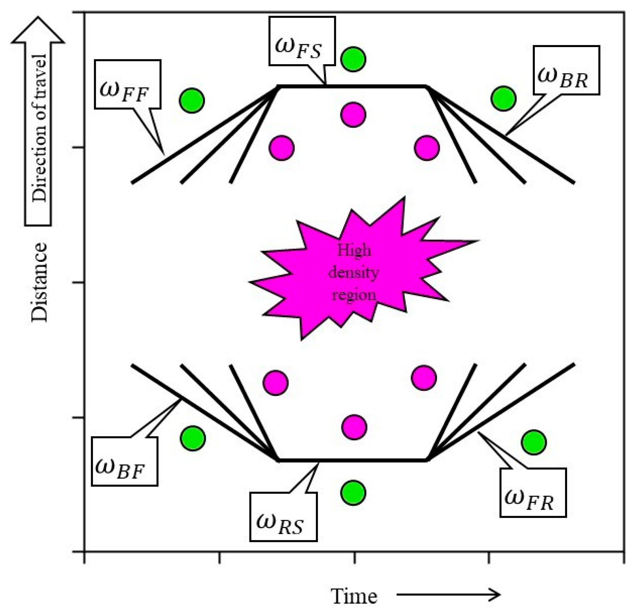
Figure 1 shows the illustration for the classification of shock waves in traffic streams in the time–space domain. The six different categories of shock waves are defined as frontal stationary (callout
), rear stationary (callout
), backward forming (callout
), backward recovery (callout
), forward forming (callout
), and forward recovery (callout
). The location of the congested or high-density region (denoted by pink circles) and the slope of the boundary between the congested and uncongested region (black lines) in the time–space domain determines the type of shock wave. The identification of shock wave type and speed is important for addressing operational questions regarding time and space locations associated with queue formation and dissipation. Backward forming shock waves on interstate highways are one of the major real-time safety concerns for transportation agencies because of the sudden change of conditions; as drivers approach, a shock wave often can cause crashes.
2. Literature Review
The theory of traffic shock waves was first proposed by Lighthill and Whitham [
1] in 1955 and utilized the method of kinematic waves. Slight changes in flow are propagated back through the stream of vehicles whose velocity is the slope of the graph of flow and density. Motorists create these waves whenever they adjust speed in accordance with the behavior of the car or cars in front of them. Researchers have used the Lighthill–Whitham (L–W) model in the analysis of bottlenecks, traffic incidents (such as a crash), a red signal light and a slow vehicle [
6,
7], which have provided sufficient characterization of the propagation of shock waves. Several techniques and analytical models were developed over the years to estimate the shock wave speed and its characteristics. A few studies have used simulation techniques to model shock waves [
8,
9,
10,
11,
12,
13,
14]. Such techniques are highly dependent on a well-calibrated simulation model which requires accurate data for inputs. The recent wide-scale availability of high-resolution connected vehicle traffic data presents a unique opportunity to measure shock wave characteristics which previously have only been represented by models. More recently, trajectory-based granular vehicle data have been utilized for a wide variety of applications including operational performance gains [
15], intersection safety, systemwide identification of signal retiming opportunities, work zone safety and management [
16], winter weather maintenance, asset management, etc., aiding transportation agencies.
The collection of traffic data with traditional equipment, like manual counters, inductive loops, fixed video camera system, etc., is an expensive and difficult process as it either requires a large amount of installed sensors/equipment or personnel in order to cover the entire network [
17]. Such location-specific equipment/sensors are not adequate to cover wide areas, which is particularly important for a phenomenon like shock waves that has high spatiotemporal variability. Another alternative for data collection was to use aerial photography. Satellites and manned aircraft have been used over the years for dynamic traffic data collection. These technologies provide a wide field of view and unbiased data. Aerial photography from aircrafts was used in the 1960s and 1970s to construct traffic density contour maps to aid in various traffic operations [
18,
19,
20,
21,
22]. Coifman videotaped sections of highway I-680 in California in 1996 to manually record individual vehicle positions [
23]. Time–space diagrams were presented for thirteen shock waves to analyze as part of the California PATH program. Several other studies have also used aerial photographs for the real-time detection of vehicles and the tracking of traffic shock waves [
24,
25,
26,
27,
28], though the cost of deployment restricts their practicality. Recent developments have used Unmanned Aerial Vehicles (UAV) for traffic monitoring, management, and control. Khan et al. presented an analytical methodology for the automatic identification of flow states and shock waves based on trajectories processed from UAV footage [
29]. However, UAV-based traffic analysis techniques [
30,
31,
32] are only feasible for relatively small areas and durations under 30 min due to battery life considerations. Also, vehicle position identification using camera images is a computationally intensive process.
Although these previous studies have been able to measure and characterize shock waves in the field, their large-scale and real-time applicability have been limited.
3. Paper Objective and Organization
The objective of this paper is to propose and validate techniques to analyze connected vehicle (CV) data to estimate the speed of the six different categories of shock waves shown in
Figure 1.
This paper is organized in the following manner:
Two case studies that illustrate how CV data can be used to estimate the speed and duration of each of the six shock waves shown in
Figure 1 (
Section 5).
Application of the shock wave principles to estimate shock wave speeds for 59 examples to demonstrate scalability (
Section 7).
A detailed case study of an incident, shock wave propagation, and subsequent secondary crash at the backward forming shock wave boundary, just prior to the backward recovery shock wave convergence (
Section 8).
Discussion of the value of estimating shock wave speeds in real time for traffic management centers to assess the impacted area and estimate the recovery time (
Section 9).
4. Connected Vehicle (CV) Data Description
CV data consist of timestamped latitude and longitude positions of anonymized consumer vehicles and are obtained through a third-party data provider. This provider receives its data directly from the original equipment manufacturers (OEMs). The advent of CV data has made it possible to obtain granular information of the traffic stream in real time at any location without deployment of physical infrastructure. A previous study in Indiana has shown that the overall CV penetration was 6.32% on interstates and 5.3% on non-interstate roadways in May 2022 [
33]. Previous studies have also shown several applications using CV data that are easy to scale and provide high value to practitioners [
34,
35].
The CV data are collected every 3–5 s and contain an anonymized trajectory identifier, GPS, timestamp, speed, and heading information. A waypoint is an individual vehicle’s speed and location at a given time. A trajectory is a set of time-ordered waypoints for a specific vehicle. Using similar techniques as those used with aerial photography, CV data can directly measure the shock wave and its speeds instead of modeling the traffic behavior.
5. Classification of Shock Waves
Shock waves are defined as a boundary condition in the time–space domain that marks a discontinuity in flow-density conditions. Shock waves arise due to sudden changes in the traffic conditions, such as crashes, lane closures, increases in traffic volume, weather incidents, or slow-moving vehicles. Shock wave speeds are used by practitioners to assess the rate of queue formation or dissipation on freeways.
Shock waves are classified into six different types depending on the propagation and high-density region in a space–time diagram. The next subsections present two examples to describe the six types of shock waves illustrated in
Figure 1.
The first example involves a lane-blocking incident associated with a vehicle rollover. The following four types of shock waves are computed from the data:
Frontal stationary (FS) shock wave;
Backward forming (BF) shock wave;
Rear stationary (RS) shock wave;
Backward recovery (BR) shock wave.
The second example involves a rolling slowdown operation. The following two types of shock waves are computed from the data:
5.1. Example 1(a): Frontal Stationary (FS) Shock Wave
By definition, a frontal stationary shock wave has a speed equal to zero (). Frontal stationary shock waves are always present at a bottleneck location and indicate the location where traffic demand exceeds capacity. Such a wave may be due to recurrent situations where the normal demand exceeds normal capacity during the peak period at a specific location. It can also be due to nonrecurrent situations where the normal demand exceeds reduced capacity, caused by an incident occurring at an arbitrary location and time. The term frontal implies that it is at the front of the congested region.
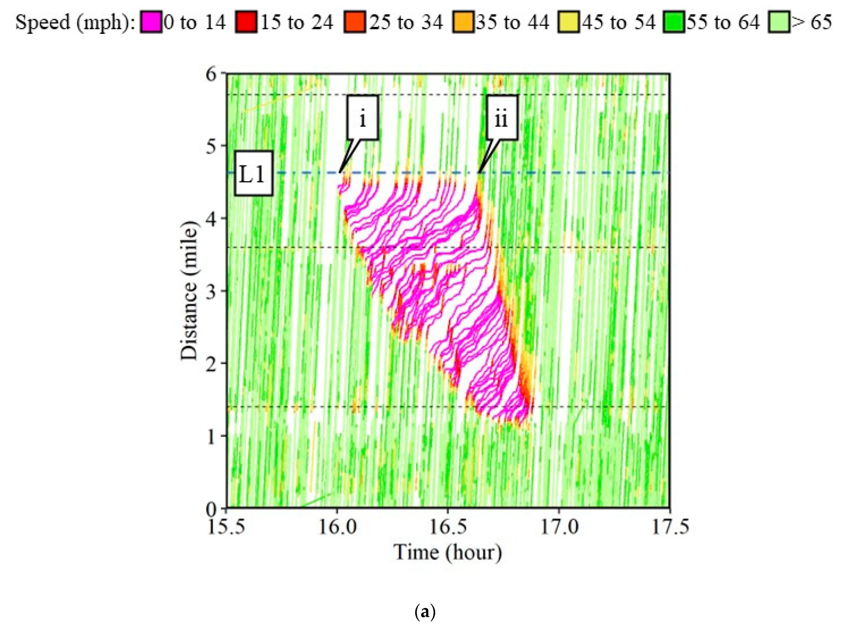
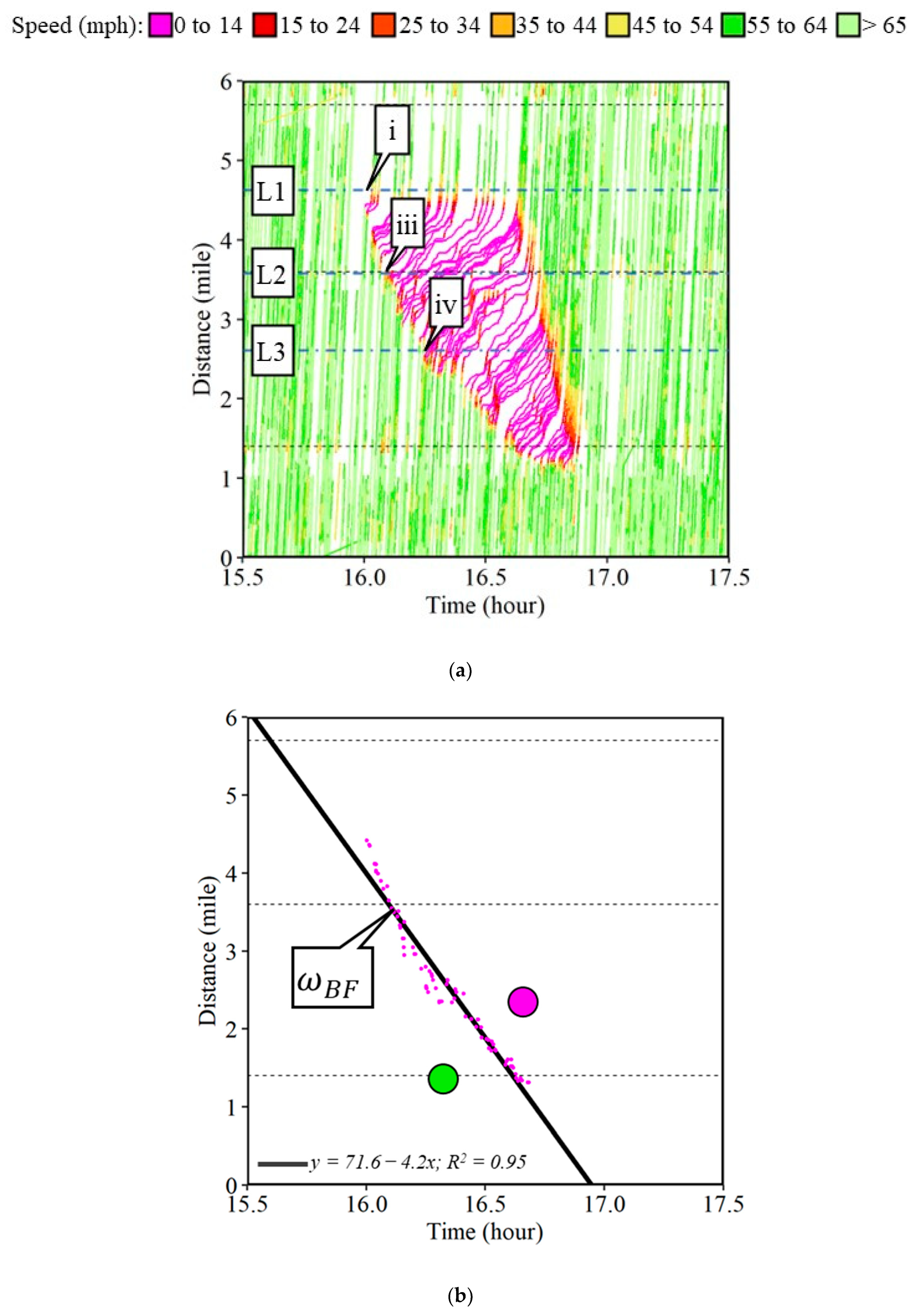
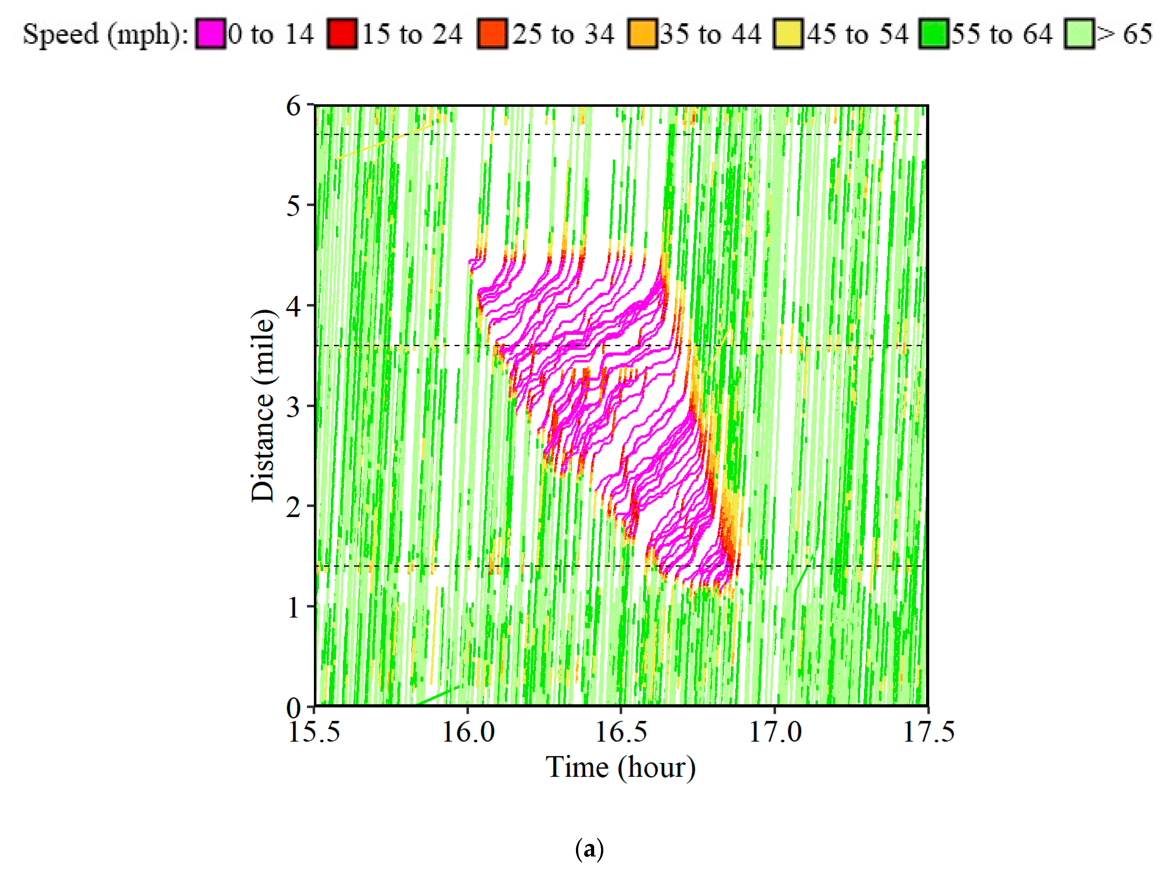
Figure 2a shows the space–time diagram of all CV trajectories along a six-mile section of the Interstate 465 (I-465) Inner Loop (IL) in Indiana for a two-hour period between 3:30 PM and 5:30 PM on Sunday, 16 January 2022. The individual waypoints for the respective trajectories are connected to each other and color-coded by the speed bins. The horizontal axis represents the time and the vertical axis shows the distance. The horizontal black dotted lines denote the locations of the interstate exists. Waypoints registering a speed below 15 mph are assumed to be in the congested region highlighted in pink. The high-density region was formed due to the incident caused on the interstate shown by callout i in
Figure 3b, with its respective location in
Figure 2a.
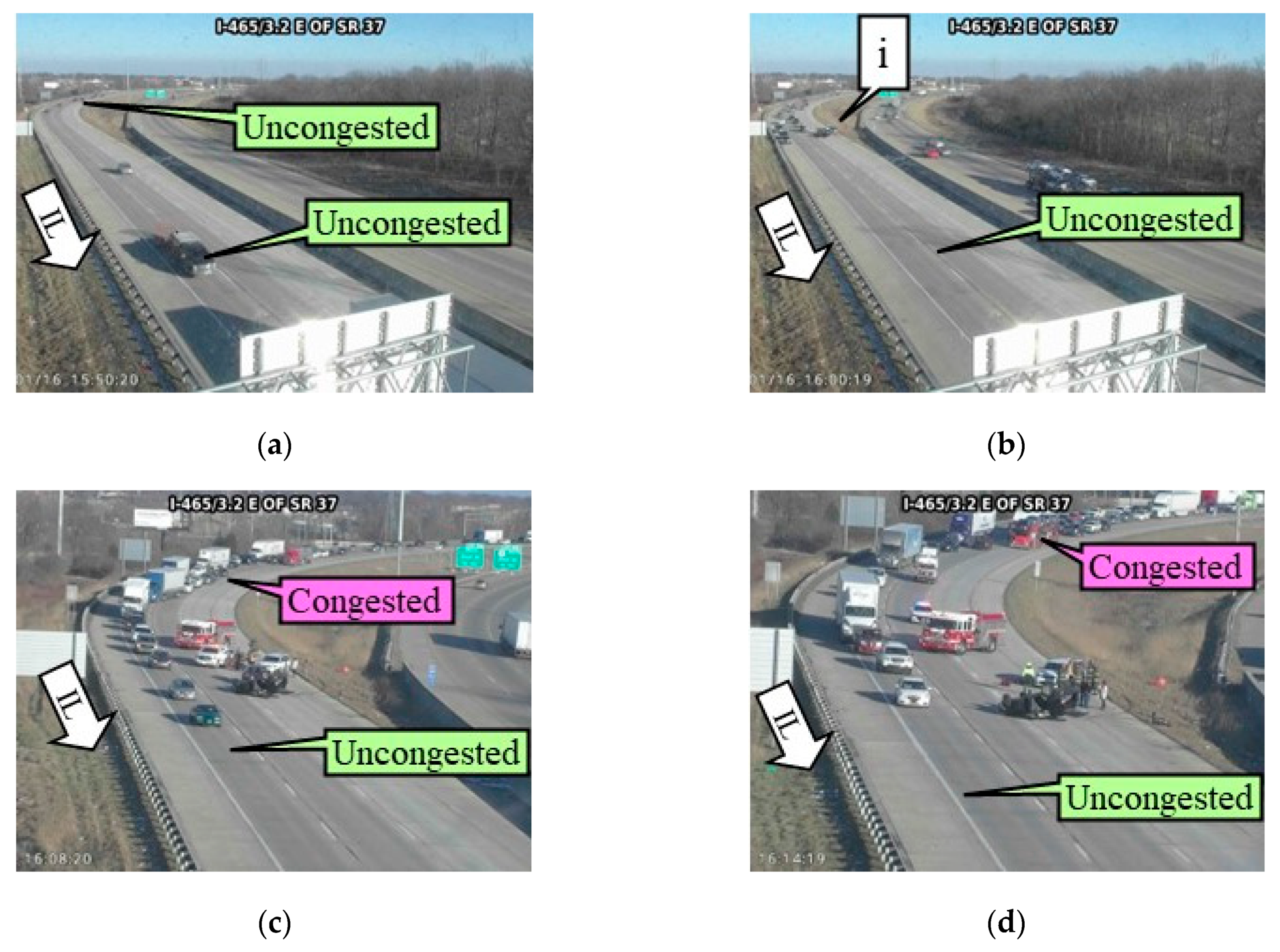
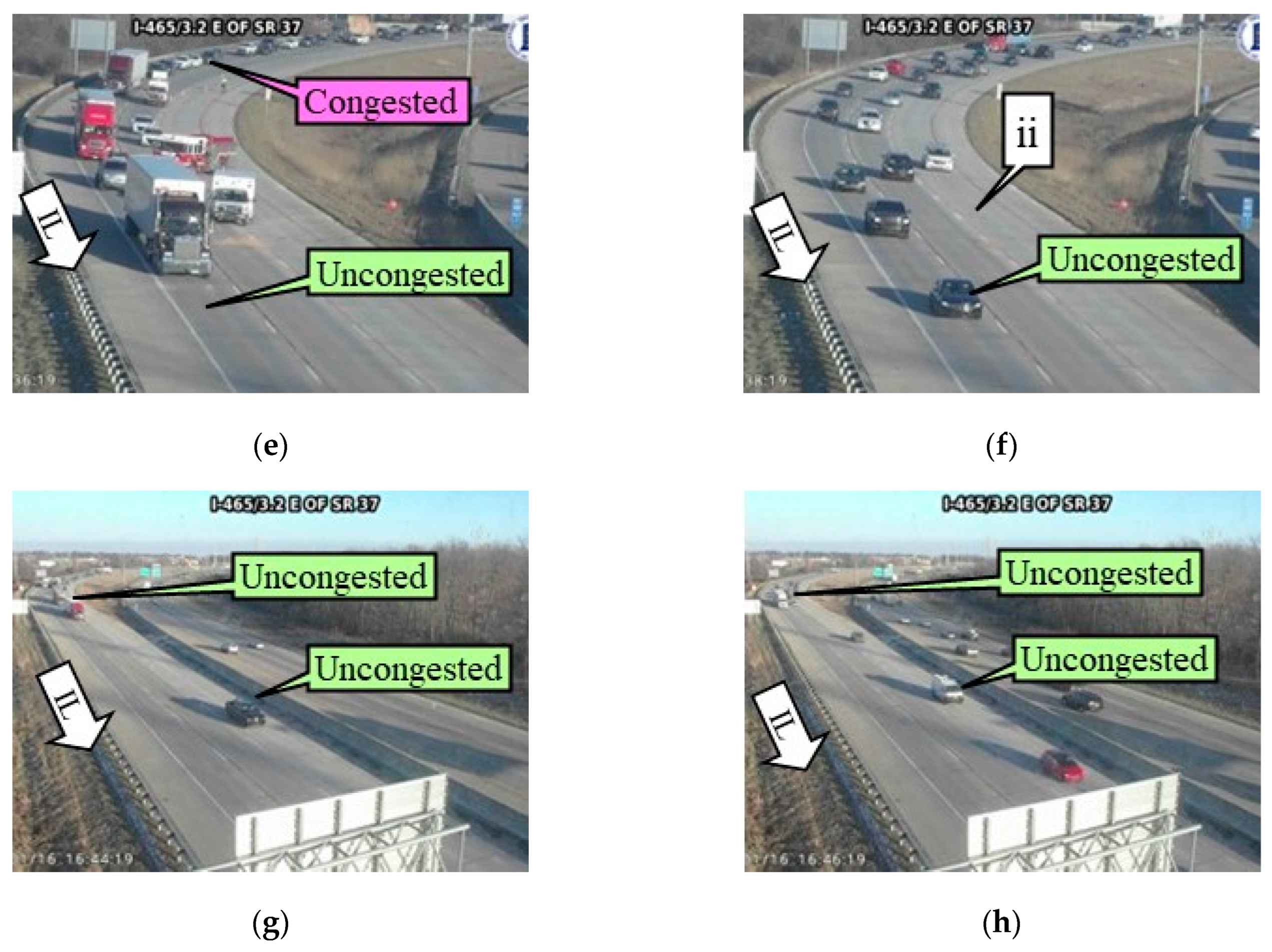
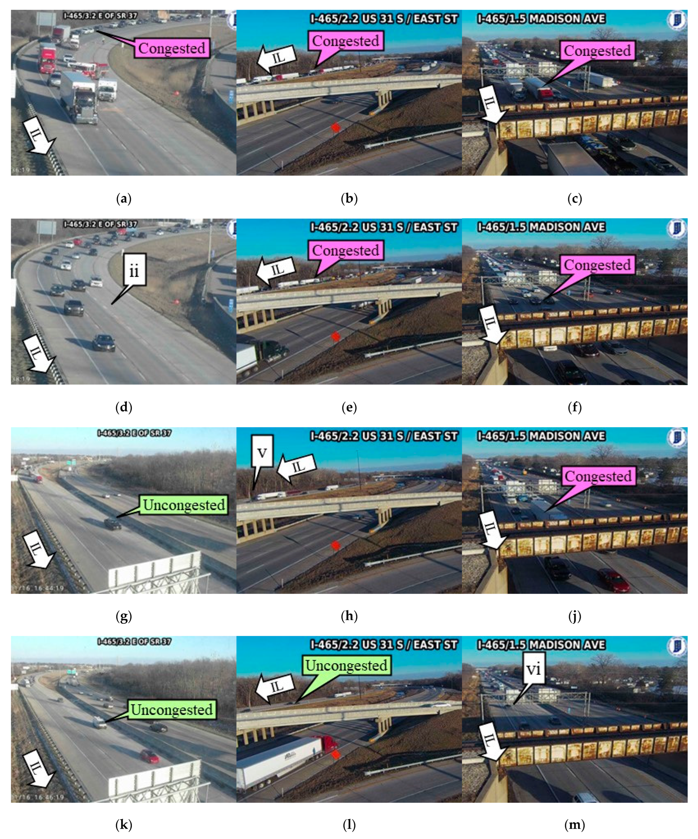
Figure 3 shows a series of camera images at location L1 in
Figure 2a. More than 500 ITS cameras across state highways are used by the Indiana Department of Transportation (INDOT) for surveillance. Callout IL denotes the Inner Loop direction of travel. Free flow traffic, i.e., uncongested conditions, can be observed at 3:50 PM (
Figure 3a) just before the occurrence of the incident around 4:00 PM (
Figure 3b). The incident blocked the left two lanes of traffic, suddenly reducing the capacity of the interstate (
Figure 3c–e). The bottleneck created due to the partial closure of the interstate initiated the shock waves seen in the time–space diagram (
Figure 2a). Upstream of the incident location, traffic is congested whereas it is uncongested downstream of the incident location. The incident was cleared and traffic started to flow freely after 4:38 PM (callout ii in
Figure 2a and
Figure 3f).
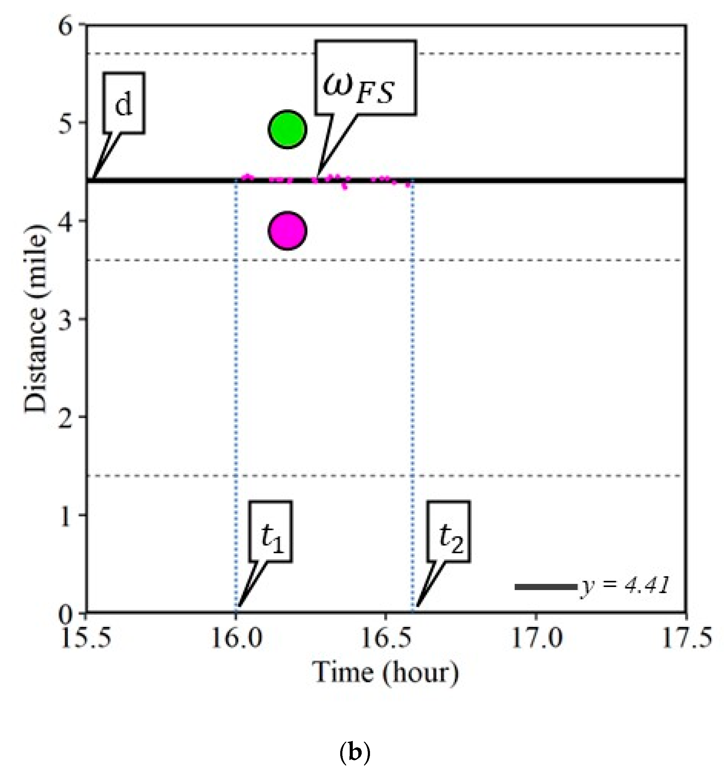
Individual waypoints from CV data with speeds below 15 mph are used for the identification of the bottleneck location, the formation of the shock wave, and the corresponding attributes of the shock waves. In the case of the frontal stationary shock wave, the latest waypoints with speeds below 15 mph before the incident clearance are chosen. When drivers turn their vehicles off, the key-off event creates separate short duration journeys within the queue, for the same vehicle, which are filtered. When information regarding the incident clearance is not available, a difference in the distance of more than 0.1 miles, i.e., the distance traveled by a vehicle travelling at 70 mph in 5 s, can be used as a limiting threshold. Twenty-two such waypoints were identified as shown by the pink dots in
Figure 2b. The average of the distances of all such waypoints gives the location of the bottleneck (callout d), with the horizontal line denoting the frontal stationary shock wave (
) estimated at distance mark 4.41. The earliest and latest waypoints at this location would roughly provide the start (callout t
1) and the end (callout t
2) of the frontal stationary shock wave. The green circle and pink circle represent the uncongested and congested regions. The schematic presented in
Figure 1 for the frontal stationary shock wave (
) closely matches the on-scene CV data in
Figure 2b.
5.2. Example 1(b): Backward Forming (BF) Shock Wave
By definition, a backward forming shock wave has a speed less than zero (
). Backward forming shock waves must always be present if congestion occurs and indicates the area in the time–space domain where demand exceeds capacity. The term backward means that over time the shock wave is moving in the opposite direction of traffic. The term forming implies that over time the congestion is gradually extending upstream. This is illustrated by the time–space domain at callout
in
Figure 1: to the left and below this shock wave has lower densities, i.e., uncongested conditions, and to the right and above, the density levels are higher, i.e., congested traffic conditions.
The case study shown In
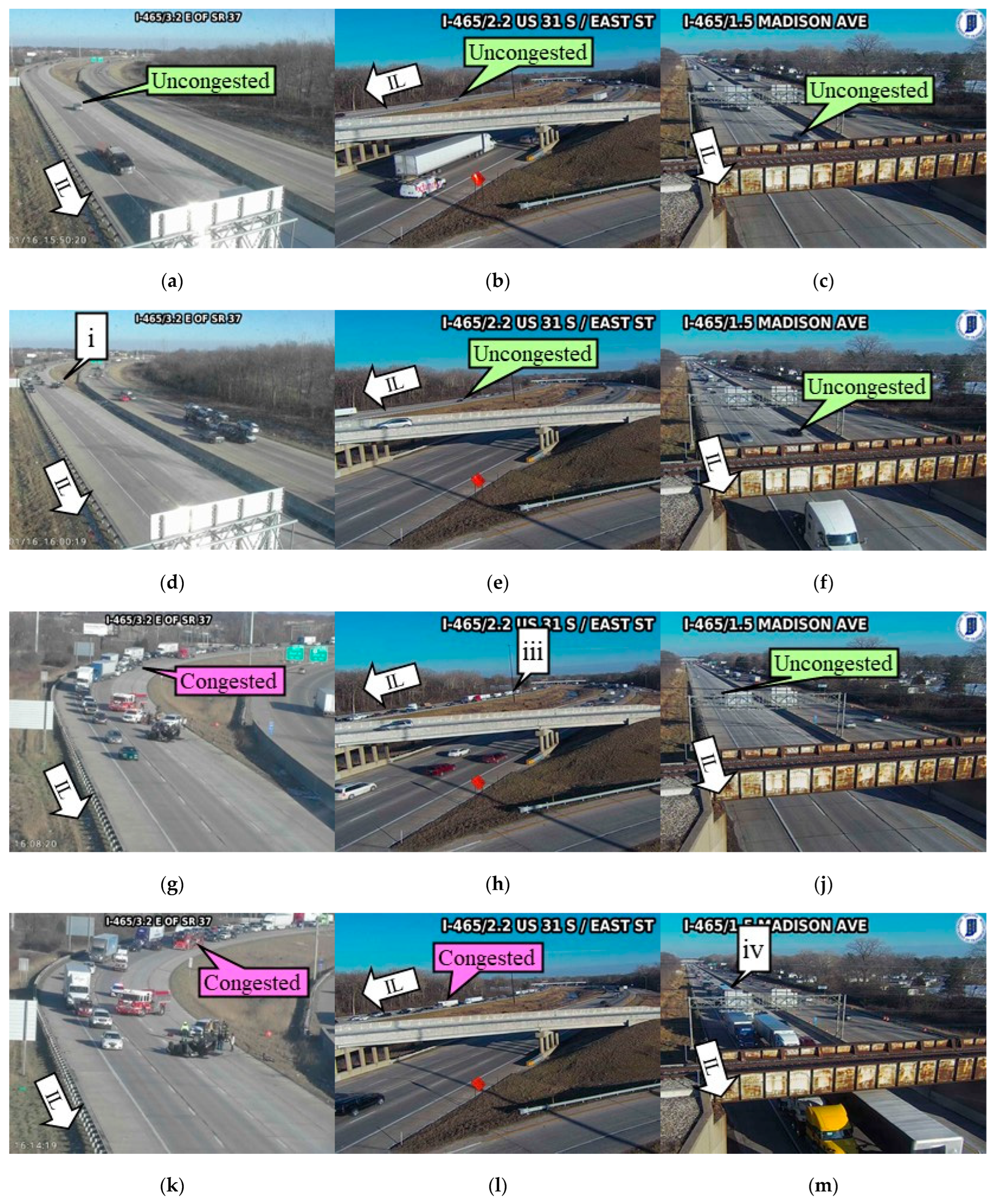
Figure 2a also shows a backward forming shock wave. Additional camera images from three different locations denoted by L1, L2, and L3 (
Figure 4a) are shown in
Figure 5. Callout iii and callout iv point to the back of the queue at locations L2 and L3 as the queue is building.
In case of a backward forming shock wave, the first waypoints with speeds below 15 mph are selected. Any waypoints that are not related to the backward forming queue are filtered. Eighty such waypoints were identified in this case shown by pink dots in
Figure 4b. A linear regression model was fitted through these waypoints. The slope was estimated as negative 4.2 mph for the linearly regressed line with a coefficient of determination (R
2) value of 0.95, showing a strong fit. The negative sign indicated that with time the shock wave is propagating upstream, opposite to the direction of traffic flow. For the backward forming shock wave, the congested region is on the right (denoted by the pink circle) and the uncongested region on the left (denoted by the green circle) in the time–space diagram. The propagation velocity for a backward forming shock wave of 4.2 mph means that every 1 hour of additional clearance time would increase the queue length by 4.2 miles. It is assumed that the backward forming shock wave has a constant speed. As the queue starts forming, the traffic tends to take alternate available routes and the traffic flow rate changes at the interstate exit locations. These exits are denoted by black horizontal dotted lines. It is important to note that, if a low R
2 value is observed for the linear regression model, the identified waypoints can be divided at the interstate exits, and separate linear regression models can be fitted at each link to identify shock wave speeds downstream and upstream of such exit locations separately.
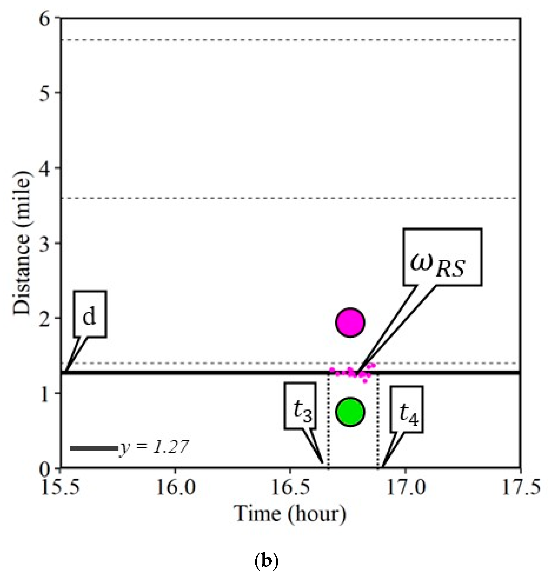
5.3. Example 1(c): Rear Stationary (RS) Shock Wave
By definition, a rear stationary shock wave has a speed equal to zero (). A rear stationary shock wave may be encountered when the arriving traffic demand is equal to the flow in the congested region for some period of time. Rear stationary shock waves might not be encountered for every instance of sudden change in the traffic and are not very common.
A rear stationary shock wave was observed for a short duration along the I-465 (
Figure 6a). Waypoints that registered a speed below 15 mph were used. Instead of using the latest waypoint as in the frontal stationary shock wave case, the earliest waypoint for every trajectory below the speed threshold was selected that was around the location of the stationary backend of the queue. Seventeen such waypoints were observed and are shown by pink dots in
Figure 6b. The average distance would give the location of the rear stationary shock wave denoted by callout d, estimated at distance mark 1.27. The minimum and the maximum timestamp of the selected waypoints provide the estimate of the start (callout t
3) and end (callout t
4) of the rear stationary shock wave. The span between the horizontal line of the rear stationary shock wave and that of the frontal stationary shock wave is the location of the congested or high-density region indicated by a pink circle.
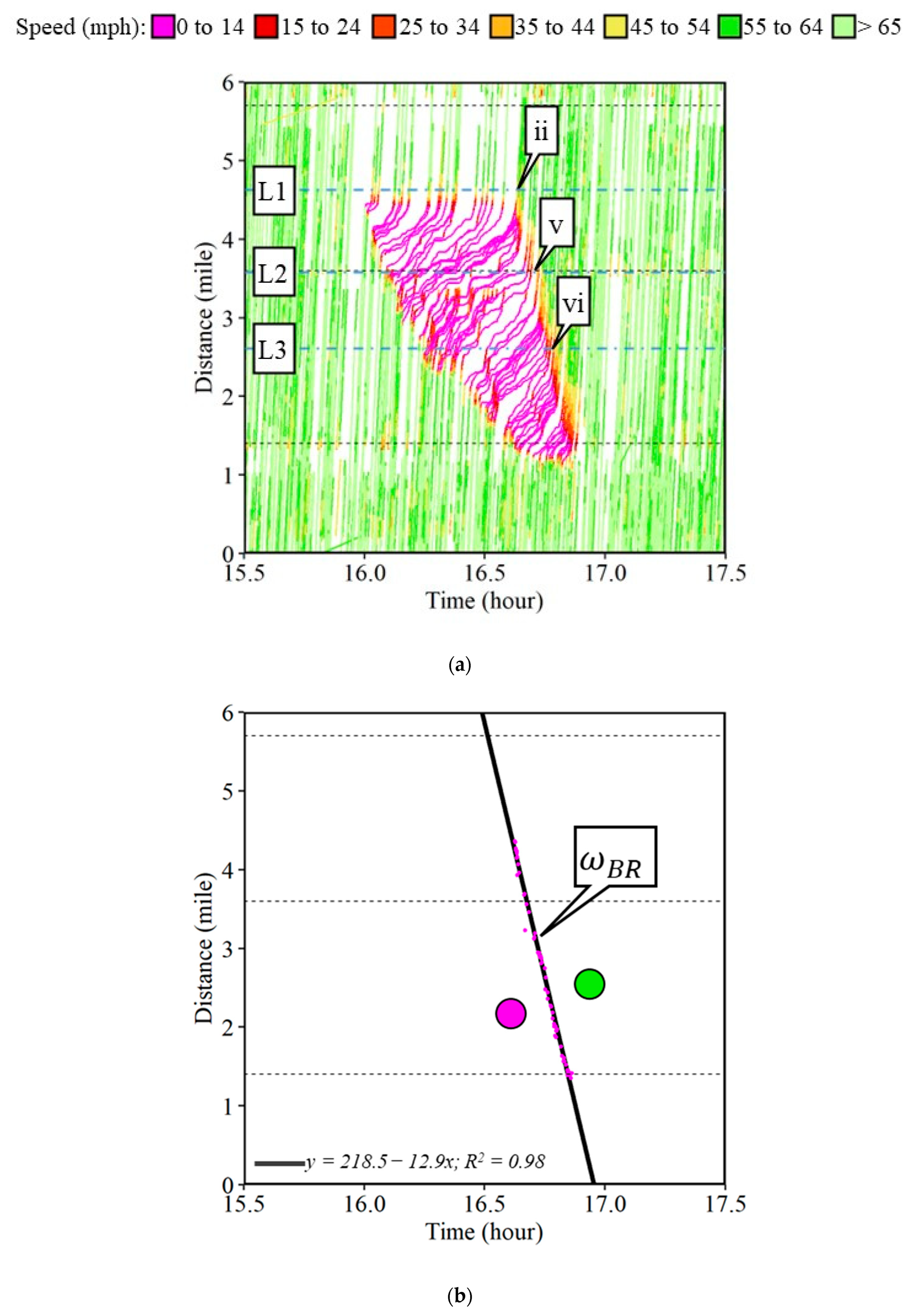
5.4. Example 1(d): Backward Recovery (BR) Shock Wave
By definition, a backward recovery shock wave has a speed less than zero (). A backward recovery shock wave is encountered when congestion has occurred but then due to increased capacity at the bottleneck after the clearance, the discharge rate exceeds the flow rate within the congested region. The term backward means that over time the shock wave is moving backward or upstream in the opposite direction of the traffic. The term recovery implies that over time free-flow conditions are extending upstream from the previous bottleneck location.
The incident along the I-465 is used to estimate the backward recovery shock wave in
Figure 7a. As soon as the incident cleared (callout ii), the roadway returned to normal capacity and created the recovery shock wave. A series of camera images from locations L1, L2, and L3 in
Figure 8 show the traffic recovery. The last waypoints with a speed less than 15 mph for every trajectory after the reopening of the entire interstate are selected for the identification of the backward recovery shock wave. Sixty such waypoints were identified, shown by pink dots in
Figure 7b. A linear regression model was fitted with a slope of negative 12.9 mph and an R
2 value of 0.98. The difference between the negatively slopped fitted regressed backward recovery shock wave and the backward forming shock wave is the location of the congested region (denoted by a pink circle). For the backward recovery shock wave, the congested region is on the left compared to that of the backward forming shock wave. A backward recovery shock wave speed of 12.9 mph suggests that every mile of queue will be dissipated in about 4.7 minutes.
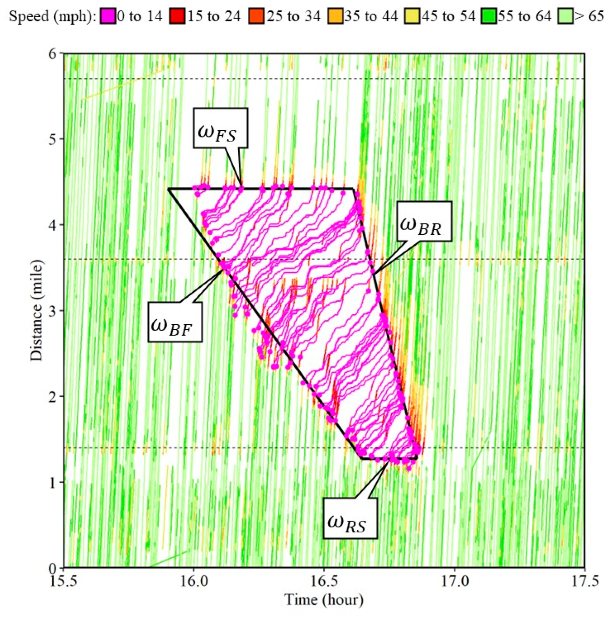
Four different types of shock waves were observed during the incident along the I-465 in Indiana.
Figure 9 summarizes the frontal stationary (callout
), backward forming (callout
), rear stationary (callout
), and backward recovery (callout
) shock waves. The individual waypoints at the boundary of the 15 mph threshold are also highlighted on top of the trajectories that were used to estimate each of the shock waves. For this incident case, the frontal stationary shock wave existed for nearly 40 min. The speed of the backward forming shock wave was 4.2 mph. The rear stationary shock wave existed for 12 min before complete recovery. The speed of the backward recovery shock wave was 12.9 mph. The queue propagation speed preliminarily depends on the traffic flow rate on the roadway and the reduction in the capacity of the roadway, i.e., full closure or partial lane closure.
5.5. Example 2(a): Forward Forming (FF) Shock Wave
By definition, a forward forming shock wave has a speed greater than zero (). Forward forming shock waves are commonly observed during rolling slowdown operations or any other slow moving vehicle such as an oversized heavy vehicle, or a maintenance vehicle impeding the traffic flow.
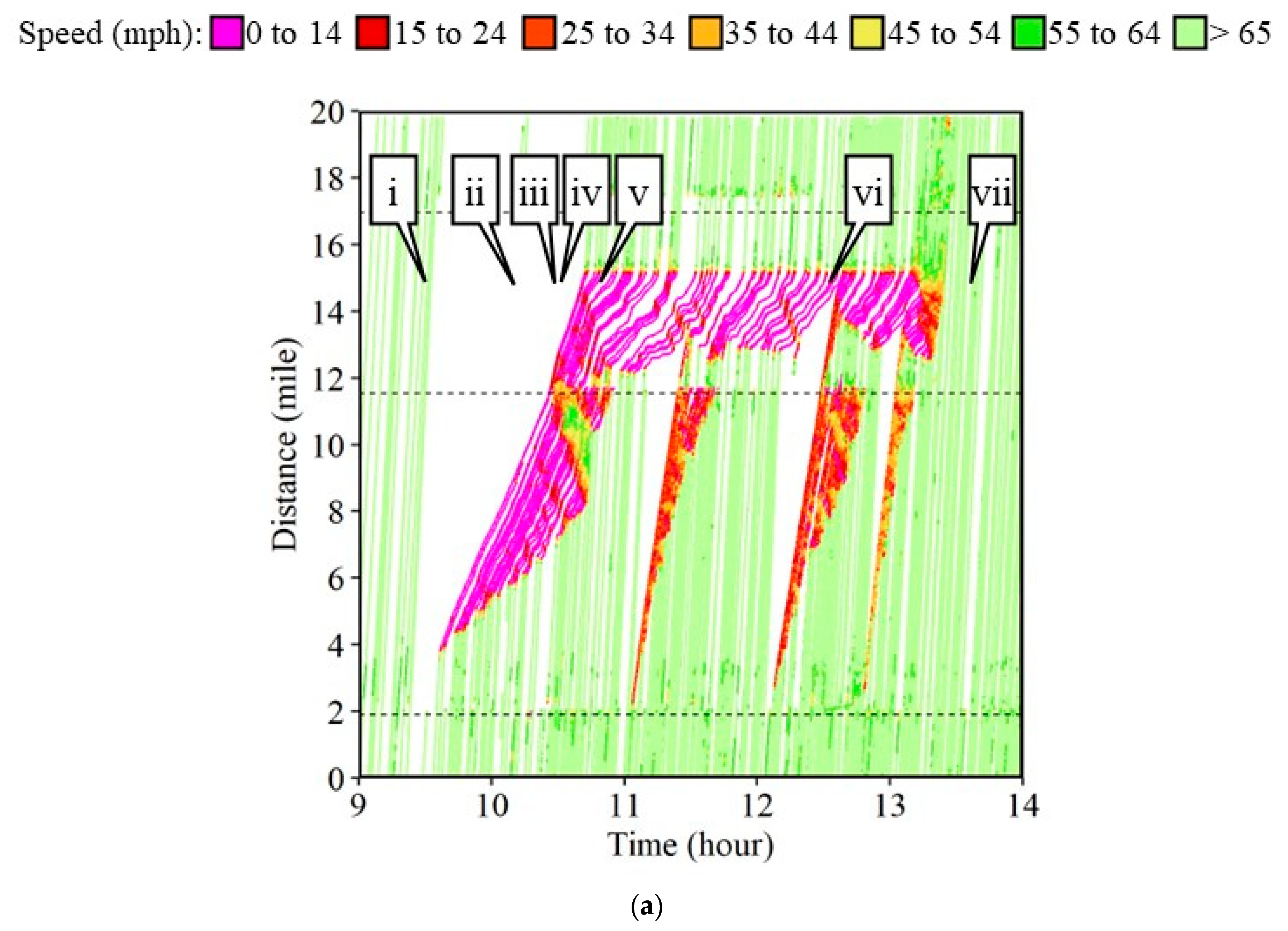
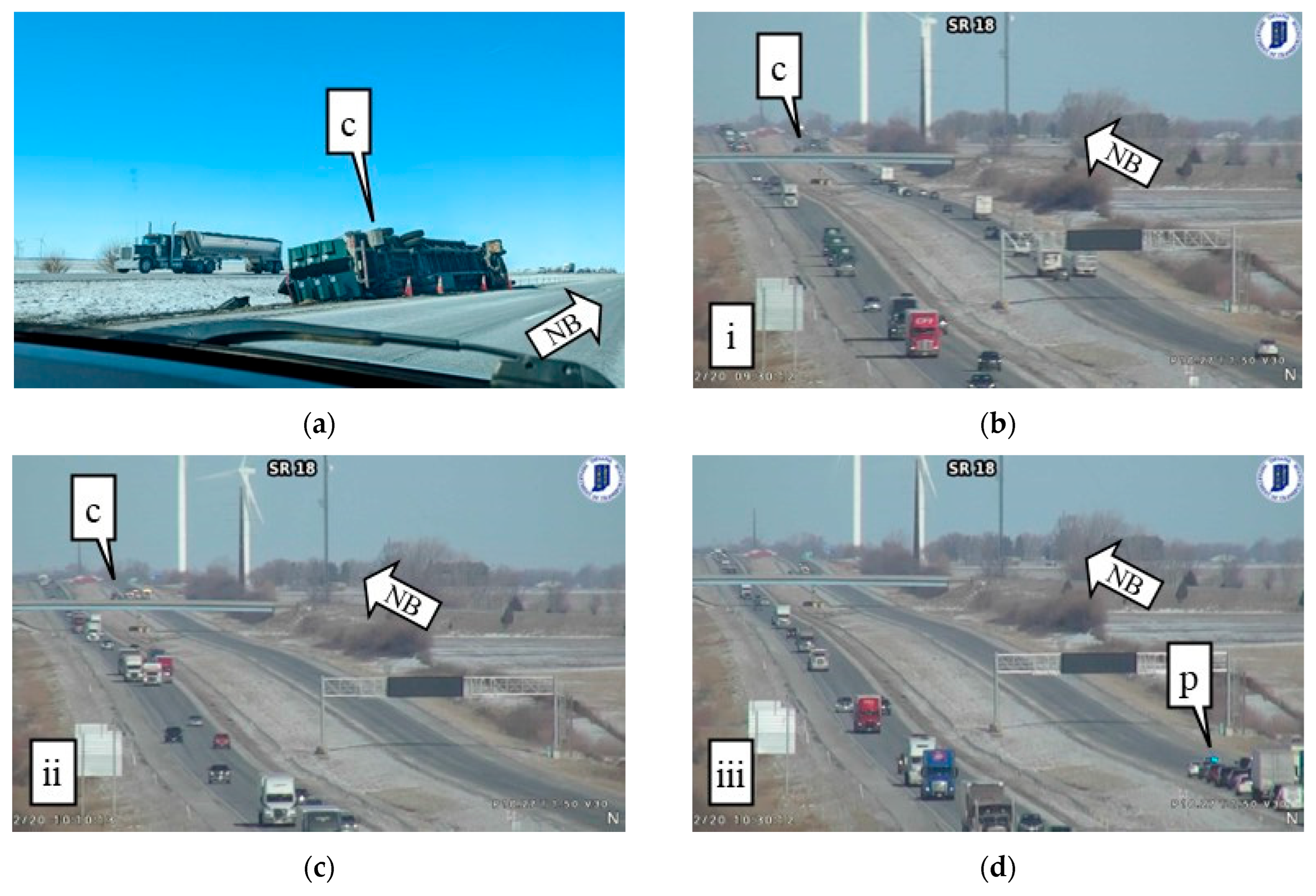
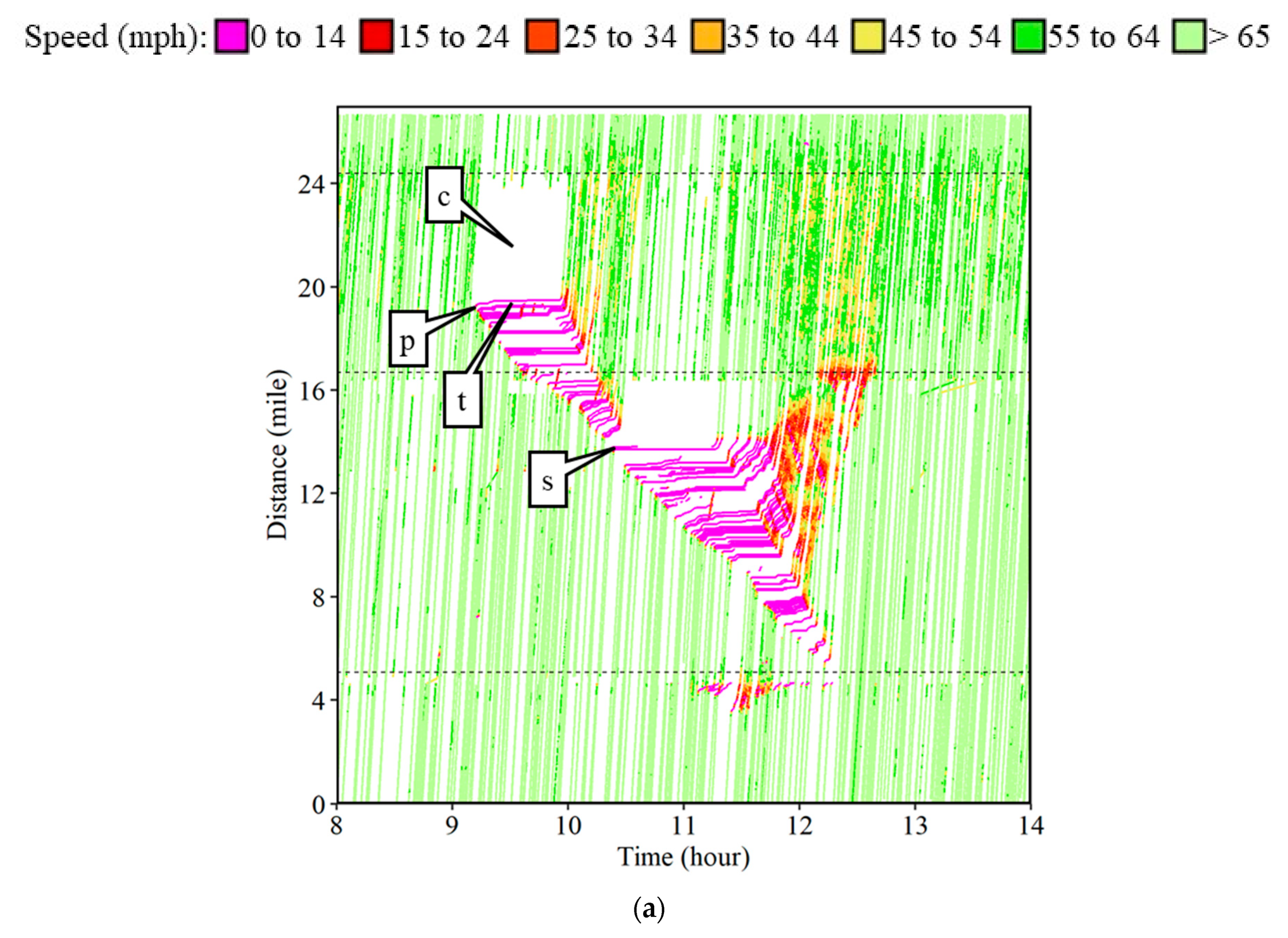
Figure 10a shows a rolling slowdown operation on the I-65 northbound (NB) direction in Indiana conducted on 20 February 2022. The operation was scheduled for clearing a truck that had rolled over during a winter storm two days prior (
Figure 11a, callout c). A patrol vehicle started to slow vehicles down shortly after it entered the interstate at mile marker (MM) 178 to MM 188 shown by the two black dotted lines around distance 2 and 12, respectively, on
Figure 10a. The patrol vehicle performed four rolling slowdown runs at various speeds.
Figure 11b–h show camera images at different times of the day near the location of the rolled-over vehicle.
Figure 11b (callout i) shows free flowing traffic when the rolled over vehicle (callout c) was still present and there were no interruptions to the traffic flow. The first run of the rolling slowdown operation started around 9:35 AM. Camera images at 10:10 AM (callout ii), 10:30 AM (callout iii), and 10:32 AM (callout iv), shown in
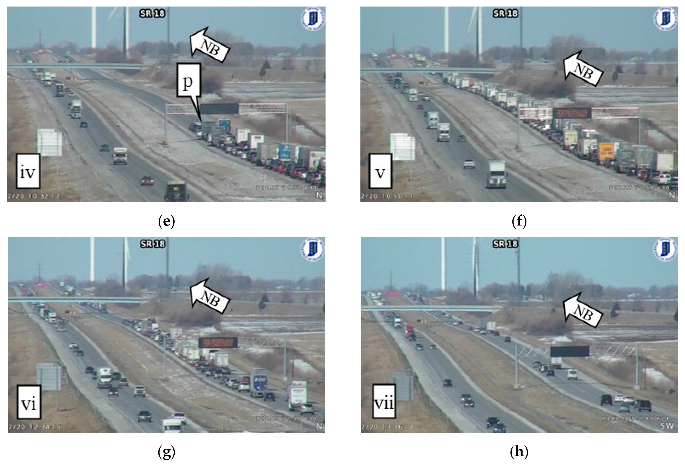
Figure 11c–e, have no flowing traffic near the location of the incident. The response vehicles working at the incident location can be observed in these images near callout c. The patrol vehicle that was conducting the rolling slowdown operation and leading the slow moving vehicles was observed in camera images at 10:30 AM and 10:32 AM in
Figure 11d,e (callout p). However, the traffic did have to slow down again as the clearance operation was not completed after the first two runs.
Figure 11e shows a camera image at 12:34 PM when it was observed that a third run of the rolling slowdown was merging with the existing congestion caused at the incident location. Traffic flow was back to normal, as seen at 1:36 PM (
Figure 11h), shortly after the completion of the fourth run of the rolling slowdown.
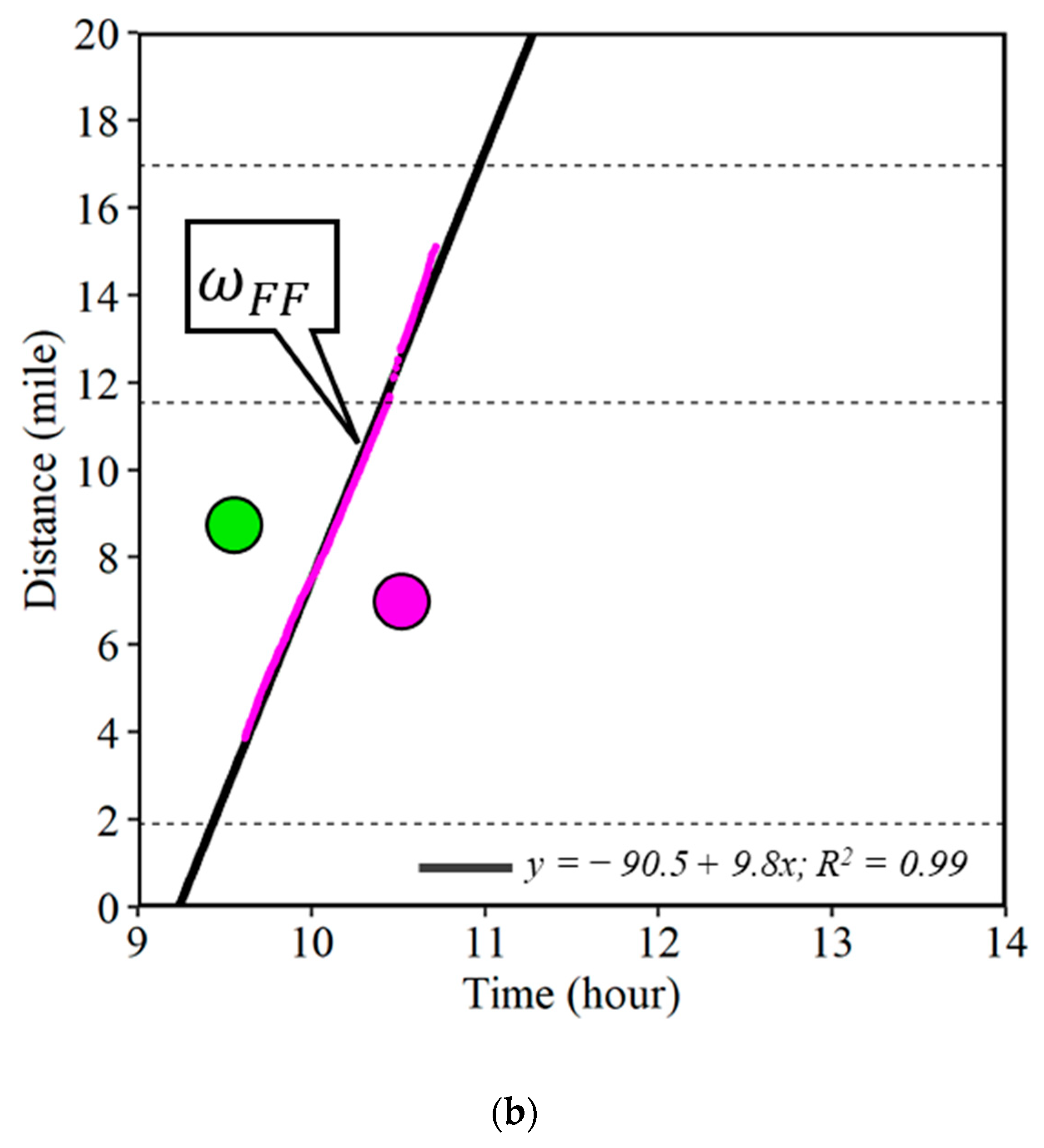
The patrol vehicle leading the rolling slowdown operation determines the speed of the forward forming shock wave. In this case, all the waypoints from the first leading trajectory are selected and shown by pink dots in
Figure 10b. A linear regressed line is fitted through these points which has a slope of 9.8 mph with an R
2 value of 0.99.
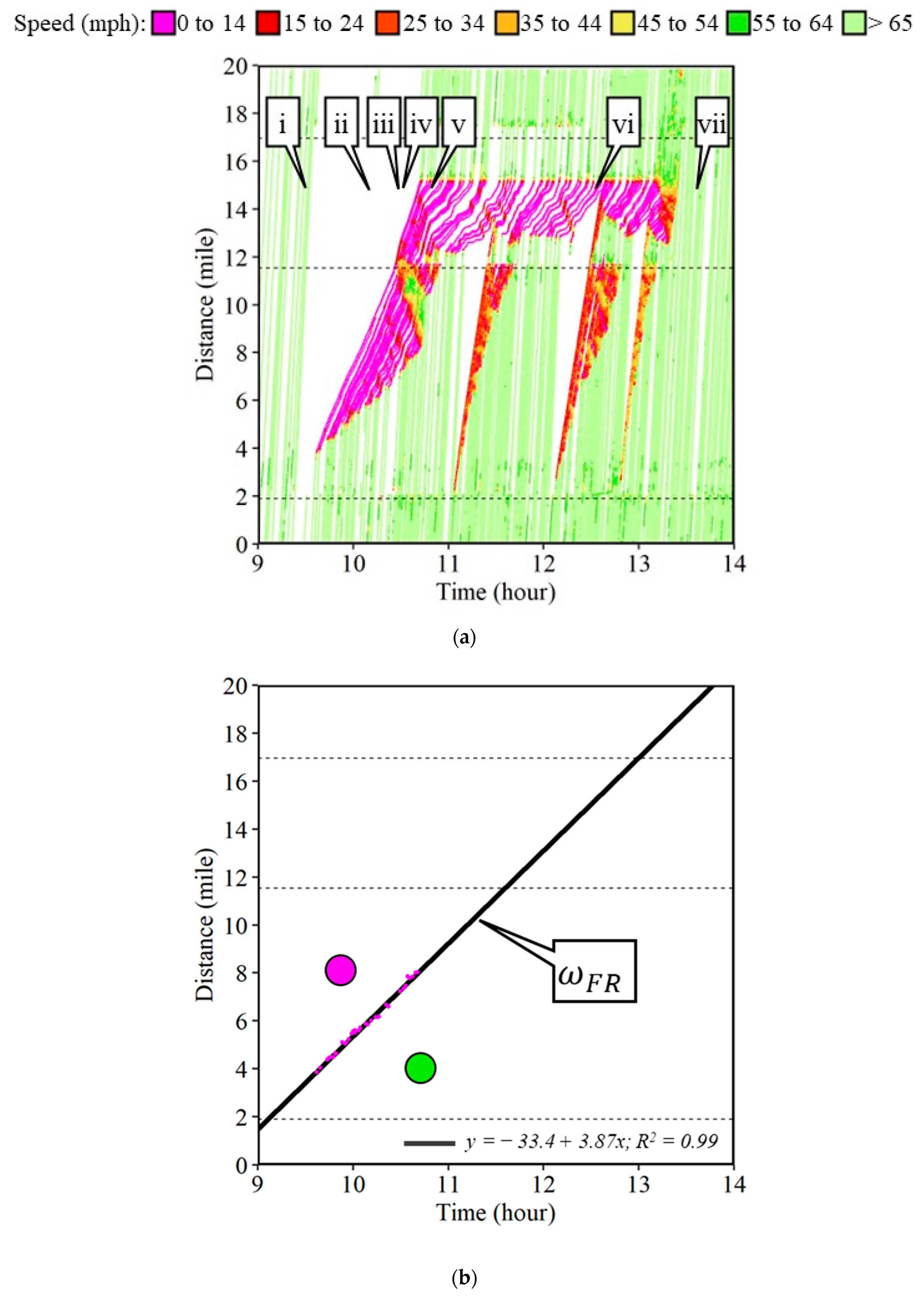
5.6. Example 2(b): Forward Recovery (FR) Shock Wave
By definition, a forward recovery shock wave has a speed greater than zero (). A forward recovery shock wave occurs when there has been congestion, but the demand decreases below the bottleneck capacity and the length of the queue is being reduced. Examples of situations where forward recovery shock waves are observed include moving operations such as a rolling slowdown or a slow-moving vehicle. The entire congestion region moves at the speed of the leading vehicle and hence the forward recovery shock wave also originates at the same time but at a slower speed compared to the slow-moving vehicle.
The rolling slowdown example from the I-65 (
Figure 12a) is also used for identifying the forward recovery shock wave. The first waypoints for the individual trajectories after the start of the rolling slowdown that have speeds below 15 mph are collected. Thirty-seven such waypoints for the first run were identified and are shown by pink dots in
Figure 12b. A linear regression model fitted through these points had a slope of 3.87 mph (callout
) with an R
2 value of 0.99. The congested region is formed between the forward forming and forward recovery shock waves.
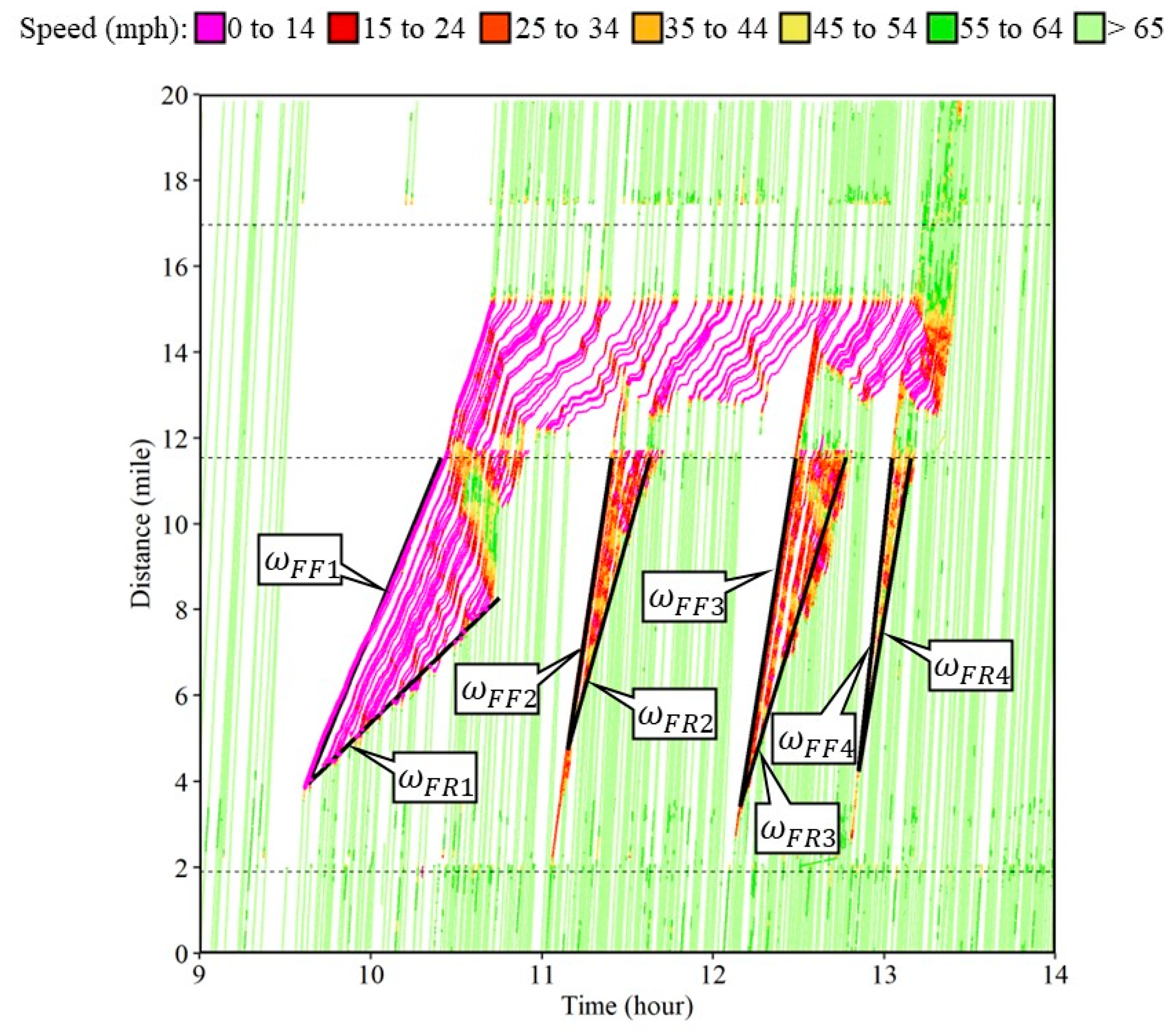
Forward forming and forward recovery shock wave speeds were also estimated for the later runs of the rolling slowdown, as shown in
Figure 13. The summary of each of the shock wave speeds is tabulated in
Table 1. The forward forming shock wave of the first run was the slowest among the four runs at 9.8 mph, and the last one was the fastest at 37.02 mph. Recovery also followed a similar trend, with the slowest recovery during the first run at 3.87 mph and the fastest recovery during the last run at 23.78 mph. The net queue formation speed is estimated as the difference between the forward forming and forward recovery shock wave speed. This will be the speed at which queues will be forming for the rolling slowdown operations. For the slower runs, a longer queue is generated. The total queue length formed for the 8-mile stretch between the two exits was 4.84 miles, 3.69 miles, 3.77 miles, and 2.86 miles for each run, respectively.
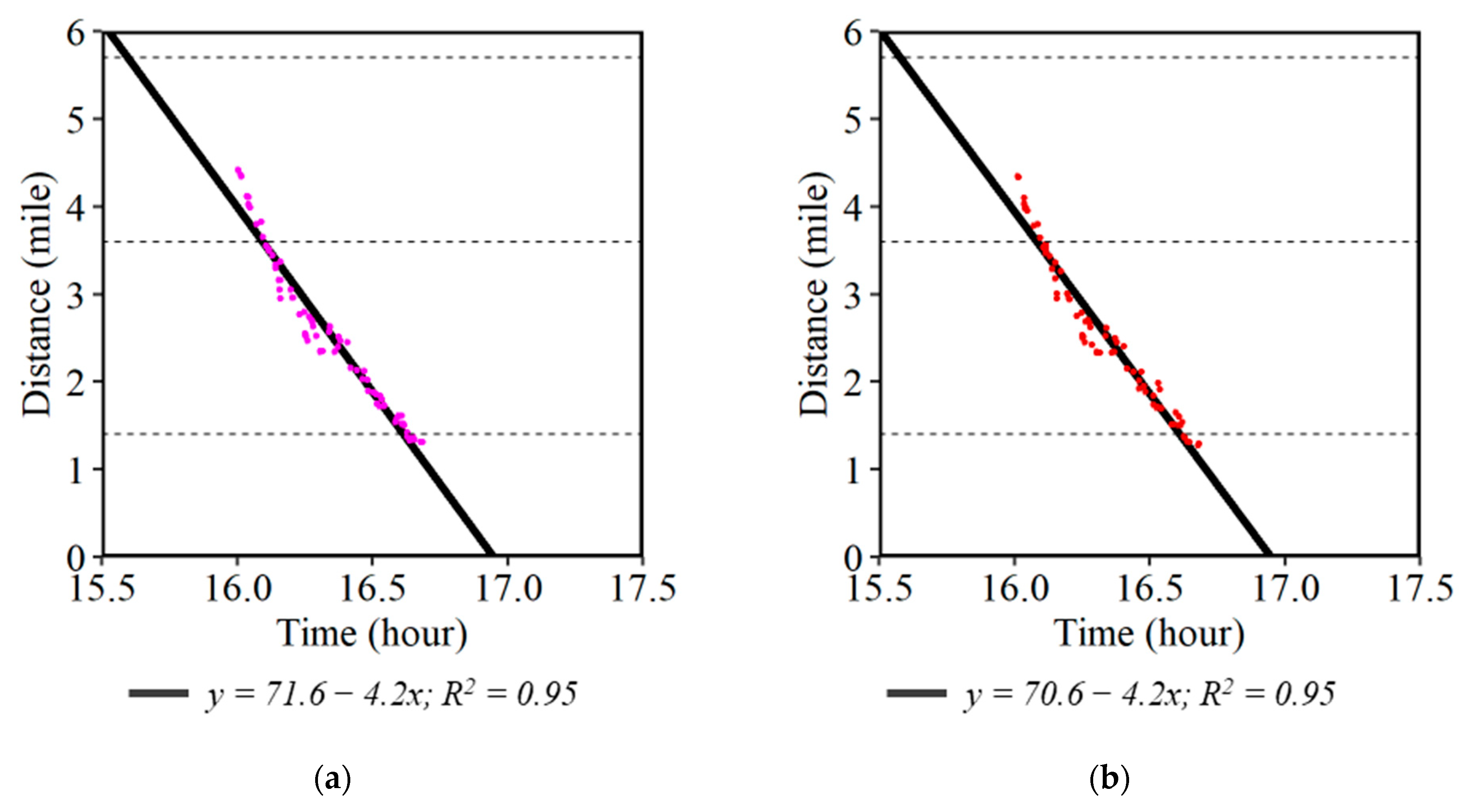
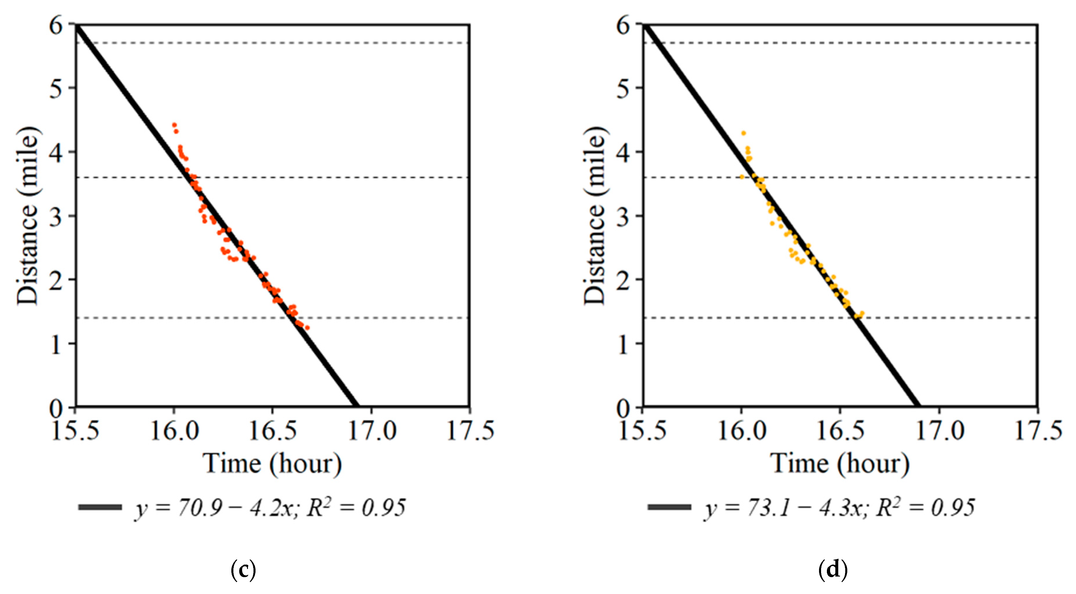
6. Sensitivity of Speed Thresholds for Estimating Shock Wave Boundaries
Some reference works, such as the Traffic Flow Fundamentals text, assume a density of 60 vehicles per lane-mile as the discontinuity boundary between the non-congested and congested flow [
2]. It is difficult to accurately measure the traffic density when 5–6% of the vehicles are providing CV data. However, it is reasonable to empirically identify this boundary by observing where and when speeds change significantly.
Figure 14 shows the estimation of backward forming shock wave speeds using four different speed boundary conditions for the same incident case shown in
Figure 4. Using a speed threshold of 15 mph or below (
Figure 14a), i.e., considering the first waypoints with speeds below this threshold at the upstream of the incident location, the estimated backward forming shock wave speed was found to be 4.2 mph. The same estimated backward forming shock wave speed using a 16–25 mph, 26–35 mph, and 36–45 mph thresholds was 4.2 mph, 4.2 mph and 4.3 mph, respectively. In all cases the R
2 value was greater than 0.95. This indicated that the choice of speed boundary threshold did not have a significant impact on the estimated shock wave speed. However, the CV data are collected at a frequency of every 3 to 5 s. If a vehicle decelerates at more than 3.3 m/s
2, the change in velocity will be more than 10 mph within the 3 s interval, and waypoints for the same vehicle might not be captured in a particular speed bin. Hence, the lowest speed threshold of 0 to 15 mph was used for selecting the boundary condition waypoints.
7. Shock Wave Speed Analysis with Varying Traffic Volumes
Fifty-nine cases of shock waves associated with incidents along three different interstates, I-465, I-65 and I-70, in Indiana were analyzed. The analysis included partial and full interstate closures for incident clearance. This analysis represents approximately 200 hours of congested conditions and used over 3.7 million connected vehicle records.
Table 2 summarizes the backward forming and backward recovery shock wave speeds for each of the cases along with the directional volume of traffic. Traffic volume data were obtained from the nearest available count station from the Indiana Department of Transportation’s (DOT’s) traffic count database system [
36] for the hour before the occurrence of the incident. It is important to note that, in some cases, the available count station was several miles away from the incident location along the same interstate. The backward forming and recovery shock wave speeds ranged from 1.75 to 11.76 mph and from 5.78 to 16.54 mph, respectively.
Traffic volume is one of the significant factors that impact the backward forming shock wave speed; however, other factors such as the type of closure, i.e., partial or full closure, the geometry, and the location of the interstate also affect the shock wave speed.
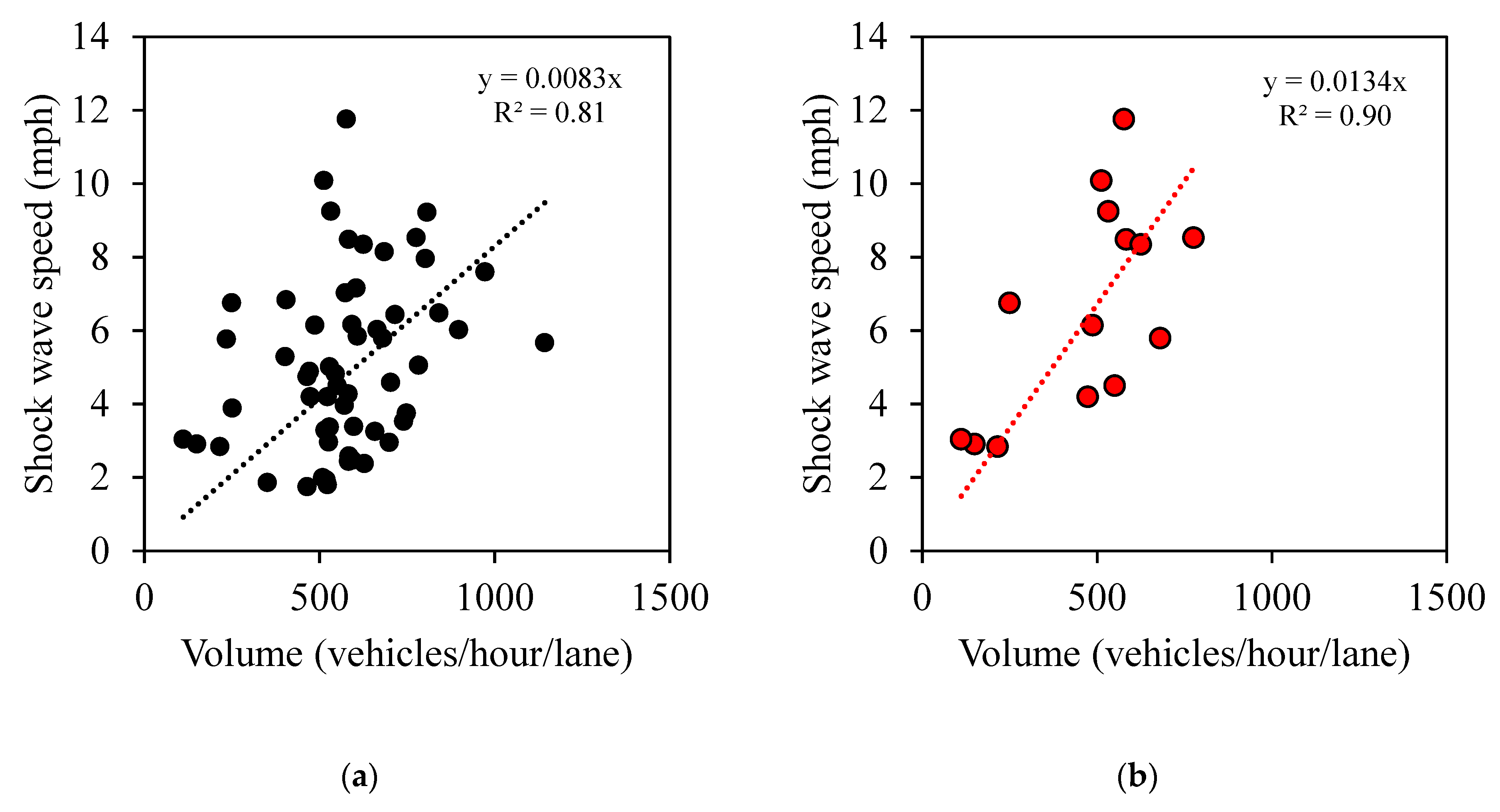
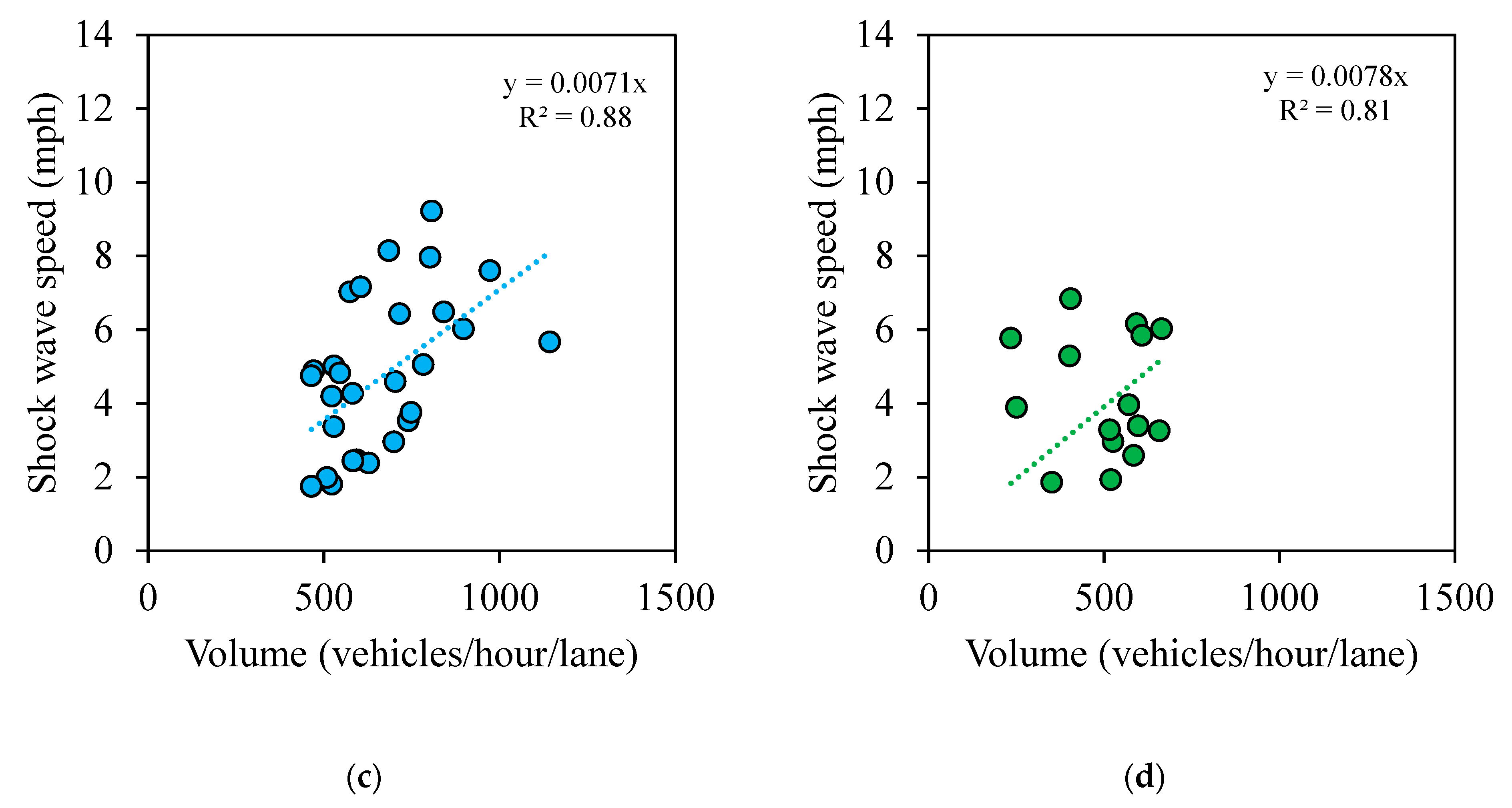
Figure 15a shows a comparison of backward forming shock wave speeds and the traffic volume for all fifty-nine cases across three interstates. Variation is observed due to other factors; however, a trend of increasing shock wave speed can be observed with an increase in traffic volume. Individual cases and the trendline for the respective interstates, I-465, I-65, and I-70, are shown in
Figure 15. The inclusion of more cases with varying volume conditions could improve the fit but, for a quick assessment, it can be assumed that every 100 vehicles per hour per lane would increase the backward forming shock wave speed by 1.34 mph on the I-465 (
Figure 15b), 0.71 mph on the I-65 (
Figure 15c), and 0.78 on the I-70 (
Figure 15d). This would help practitioners quickly gauge the length of the queue that will be formed for a given traffic volume and clearance time to plan accordingly.
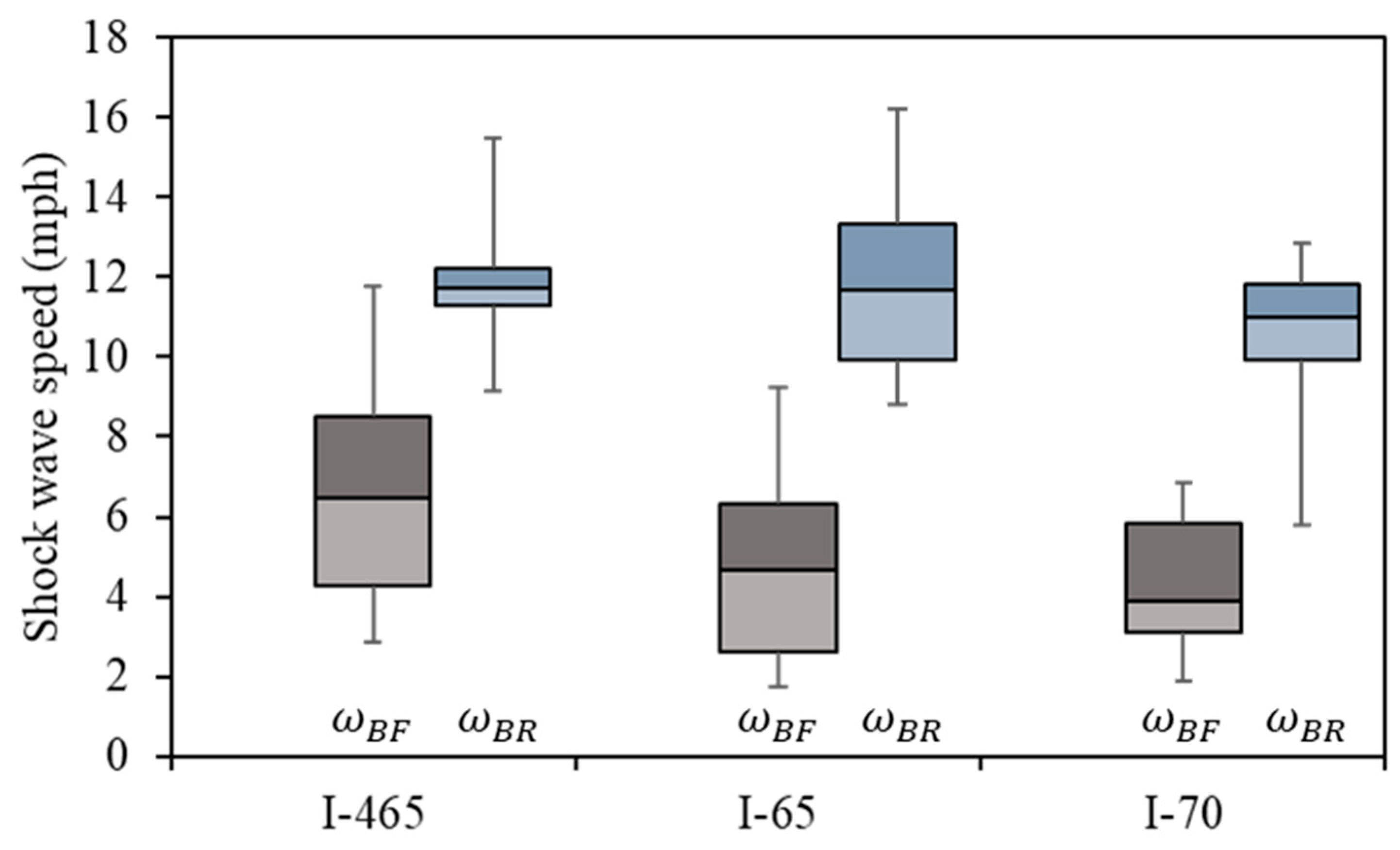
Backward forming shock wave speeds were found to have been impacted by traffic volume. Once a scene is cleared, there tends to be less variation in the shock wave speed, and it is predominantly influenced by driver distraction at the site of the incident that was cleared.
Figure 16 shows the box-and-whisker plot for both backward forming and recovery shock wave speeds by interstate. The backward forming shock wave speeds were higher along the I-465 compared to the other interstate, as was the traffic volume. The backward forming shock wave speed also did not vary much across interstates; the backward recovery shock wave speed was between 8.7 and 13.7 mph for 47 out of the 59 cases.
Some data limitations are as follows:
Traffic volume obtained from count stations might be different than the actual volume at the location and time of the incident.
Change in the number of lanes, geometry of the interstates, and/or presence of the interstate exit inside the queue region.
Presence of work zone activities or regions with reduced speed limits.
8. Application of Shock Wave Speed for Assessing Incident Response
Practitioners can utilize shock wave speeds to estimate queue formation or queue dissipation rates at specific roadways for after-action applications. Responders can estimate how long the queue will keep forming for every incremental delay in the clearance time. Traffic operators would also be able to estimate the time required for the traffic flow to get back to normal after the reopening of a route.
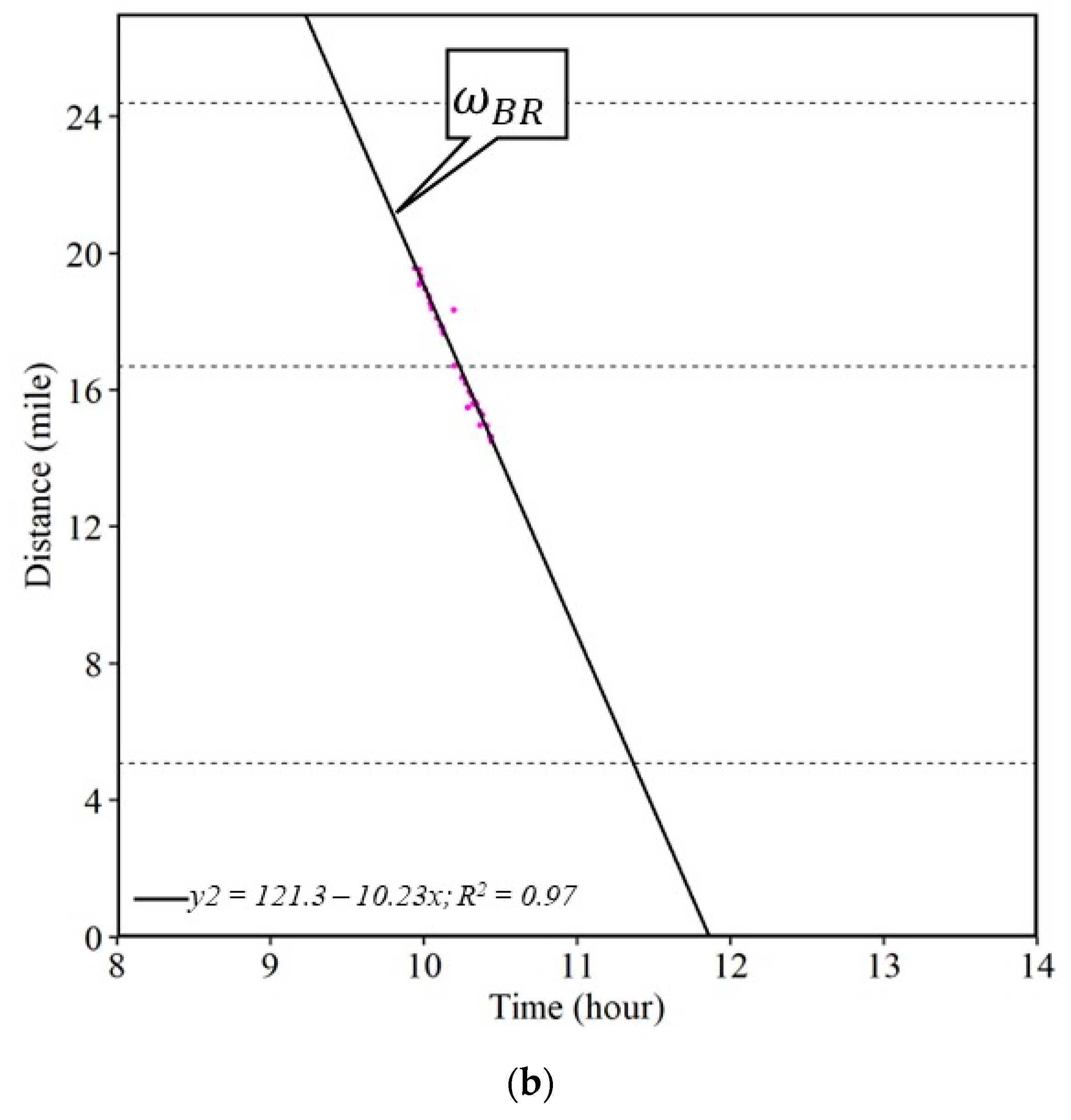
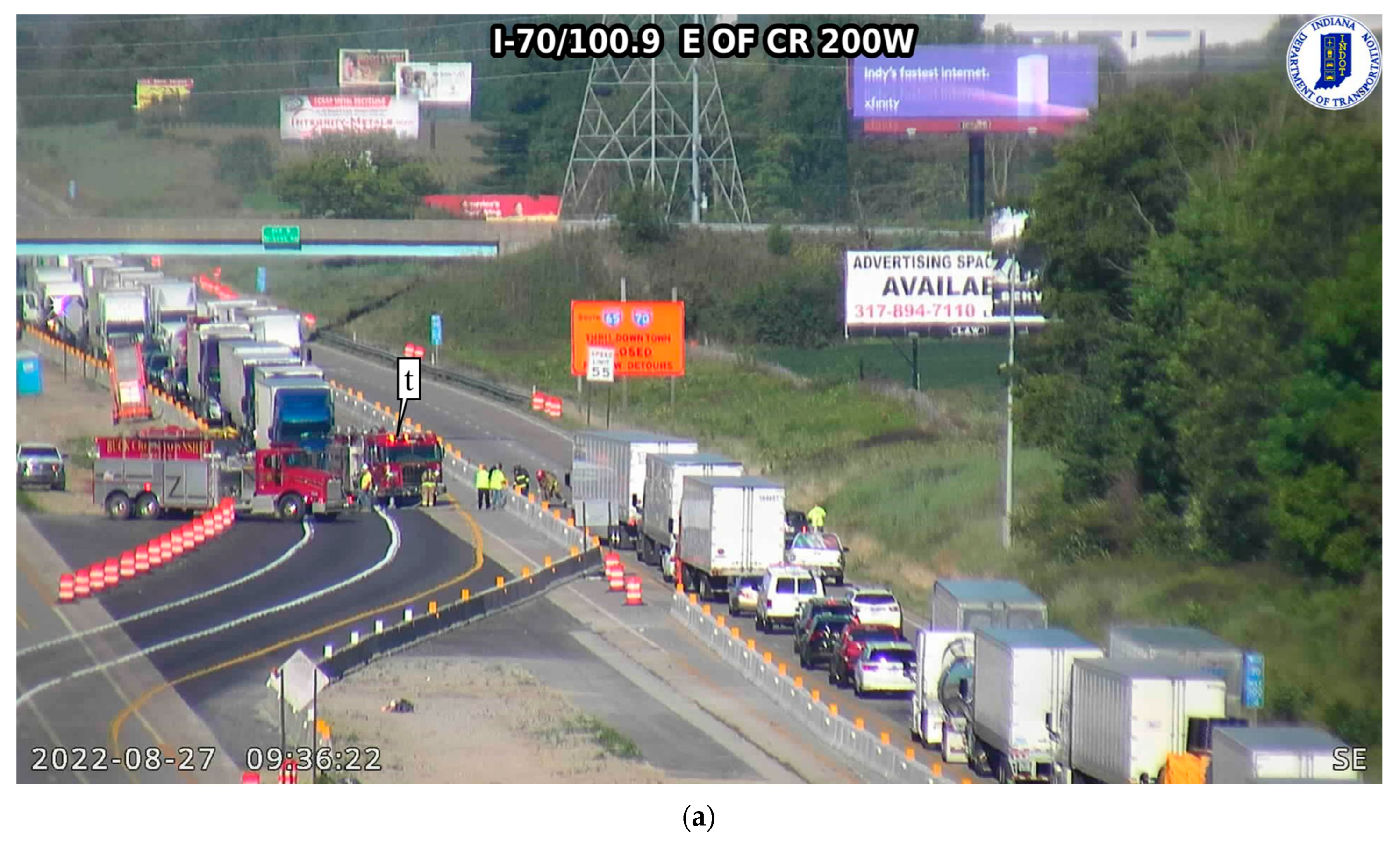
Figure 17a shows one such example of an engine fire (callout p) that caused shock waves along the I-70 on Saturday, 27 August 2022. The engine fire incident occurred around 9:08 AM and closed the eastbound interstate for about 48 min.
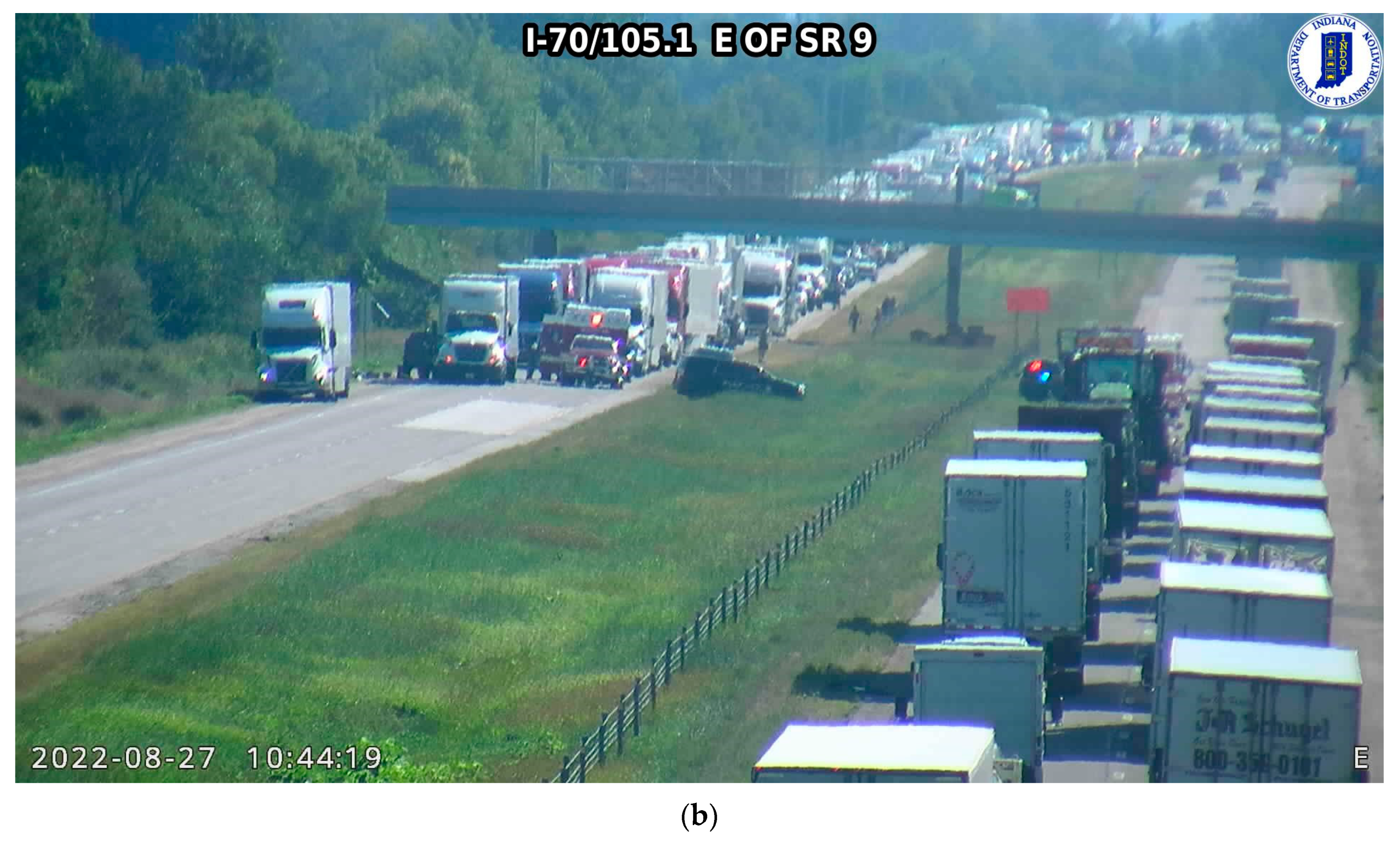
Figure 18a shows the fire trucks responding at the incident location (callout t) with stopped traffic in both directions of travel. The interstate closure can also be observed from the white patch (callout c) with no trajectories downstream of the incident location after the engine fire broke out. A secondary crash occurred, as seen in
Figure 18b, at the back of the queue around 10:15 AM, almost five miles upstream of the engine fire location (callout s). The interstate exits are denoted by black dotted lines in
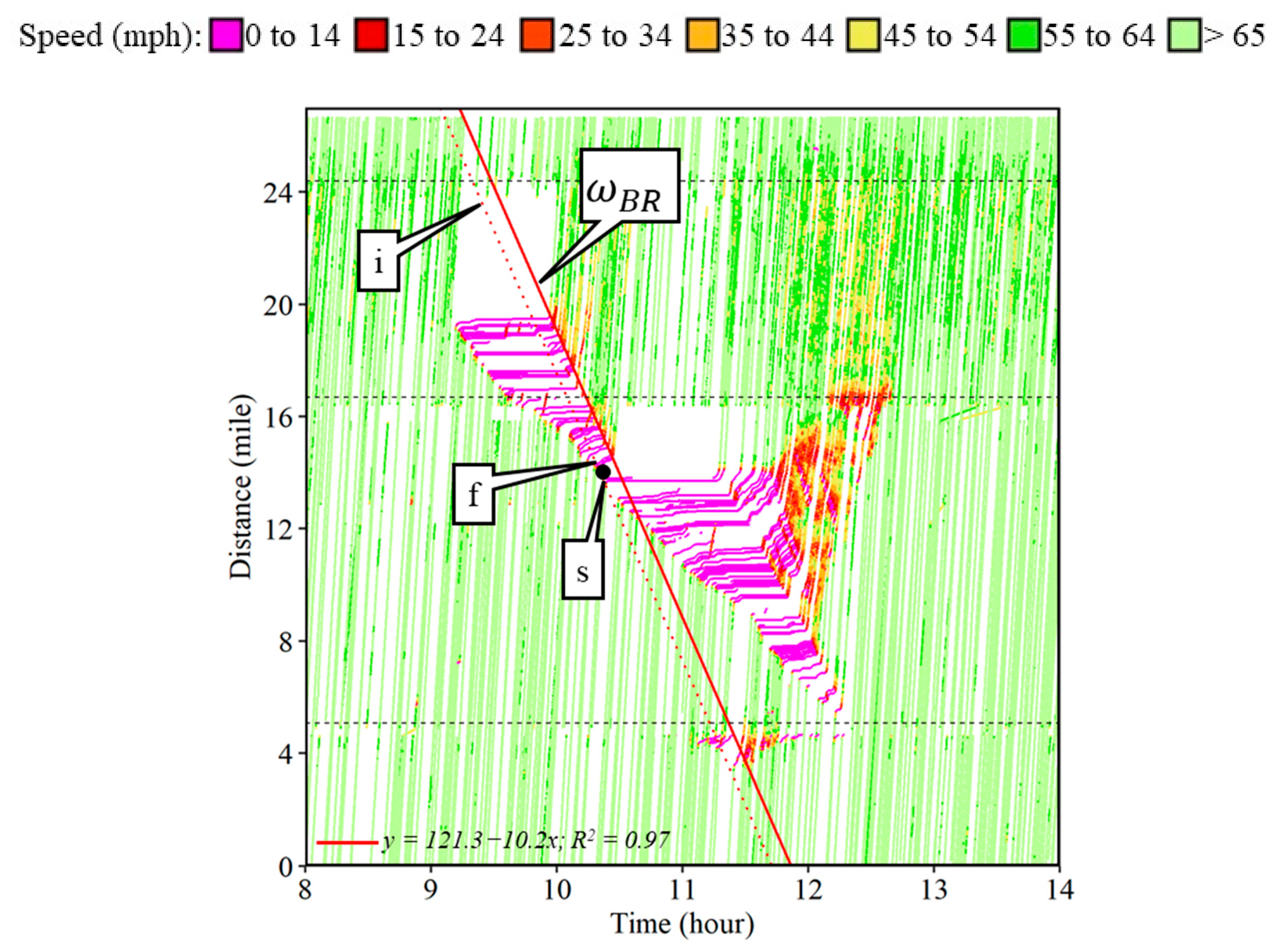
Figure 17. After the engine fire was completely extinguished and the incident was cleared, the interstate was opened back up around 9:56 AM starting the recovery shock wave. The backward recovery shock wave speed was estimated to be 10.23 mph (callout
in
Figure 17b), i.e., almost 1 mile of queue recovered every 6 min.
Figure 19 shows the backward recovery shock wave (
) overlaid on top of the trajectories. The secondary crash incident is indicated by callout s. The secondary crash incident occurred just a few minutes before the recovery had reached this location. The sooner the bottleneck is cleared, the sooner the recovery would reach the back of the queue, while the queue will also be shorter. The likelihood of a secondary crash incident at the back of the queue is then reduced.
For this case study, an early recovery by time (
t) was estimated such that the location of the secondary crash incident had free flowing conditions up to the time of the secondary incident, given by equation
where
is the early recovery time in hours,
is the time coordinate of the secondary crash incident,
is the location coordinate of the secondary crash incident,
is the intercept, and
is the slope for the backward recovery shock wave as estimated in
Figure 17b. The early recovery time (
t) was estimated to be 8.79 min. If the engine fire incident had been cleared 9 min earlier, the secondary crash incident could have been prevented. Callout i denotes the potential recovery shock wave given the interstate was reopened 9 min earlier. Callout f points to the location of free flow conditions where downstream of that location traffic would not experience any congestion.
9. Conclusions
The shock waves of three case studies involving traffic incidents along Indiana Interstates were analyzed in detail using CV data. The CV data provide an opportunity to identify and measure shock wave forming or recovery speed anywhere across the roadway network.
Typical backward forming shock wave speeds ranged from 1.75 to 11.76 mph.
Typical backward recovery shock wave speeds were between 5.78 and 16.54 mph.
The estimated backward forming shock wave speed was found to be insensitive to the choice of speed threshold.
It was also estimated that every 100 vehicles per hour per lane would increase the backward forming shock wave speed by 1.34 mph on the I-465, 0.71 mph on the I-65, and 0.78 on the I-70 in Indiana (
Figure 15).
Practitioners can use this information to quickly gauge the length of the queue that will be formed for a given traffic volume and clearance time, and plan accordingly.
The analysis of a case study involving a secondary crash showed that an estimated early incident clearance by 9 min (
Figure 19) could have prevented the secondary crash incident that occurred at the back of the queue. The capability of identifying and measuring such shock wave speeds can be utilized by various stakeholders for traffic management decision making, particularly when training first responders (fire departments, EMS, police) on the importance of minimizing lane closure times. Near real-time estimation of shock waves using CV data can recommend travel time prediction models and serve as input variables to navigation systems to identify alternate route choice opportunities ahead of a driver’s time of arrival.
Author Contributions
Conceptualization: R.S.S., H.L. and D.M.B.; Methodology: R.S.S.; Validation: H.L.; Formal Analysis: R.S.S.; Resources: H.L. and D.M.B.; Data curation: R.S.S.; Writing—original draft: R.S.S.; Writing—review & editing: D.M.B., H.L. and R.S.S.; Visualization: R.S.S.; Supervision: D.M.B. All authors have read and agreed to the published version of the manuscript.
Funding
This research received no external funding.
Institutional Review Board Statement
Not applicable.
Informed Consent Statement
Not applicable.
Data Availability Statement
Not applicable.
Acknowledgments
The connected vehicle data between January and October 2022 used in this study were provided by Wejo Data Services, Inc. The contents of this study reflect the views of the authors, who are responsible for the facts and the accuracy of the data presented herein, and do not necessarily reflect the official views or policies of the sponsoring organizations. These contents do not constitute a standard, specification, or regulation.
Conflicts of Interest
The authors declare no conflict of interest.
References
- Lighthill, M.J.; Whitham, G.B. On kinematic waves II. A theory of traffic flow on long crowded roads. Proc. R. Soc. Lond. A Math. Phys. Sci. 1955, 229, 317–345. [Google Scholar] [CrossRef]
- Adolf, D.M. Traffic Flow Fundamentals; Prentice Hall: Englewood Cliffs, NJ, USA, 1990. [Google Scholar]
- Gerlough, D.L.; Huber, M.J. Traffic Flow Theory A Monograph. Transp. Res. Board Spec. Rep. 1975, 165, 53903265. [Google Scholar]
- Richards, P.I. Shock Waves on The Highway. Oper. Res. 1956, 4, 42–51. [Google Scholar] [CrossRef]
- Stephanopoulos, G.; Michalopoulos, P.G.; Stephanopoulos, G. Modelling and analysis of traffic queue dynamics at signalized intersections. Transp. Res. Part A Gen. 1979, 13, 295–307. [Google Scholar] [CrossRef]
- Wirasinghe, S.C. Determination of traffic delays from shock-wave analysis. Transp. Res. 1978, 12, 343–348. [Google Scholar] [CrossRef]
- Edie, L.C. Flow theories. Traffic Sci. 1974, 1–108, (Edited by Gazis, D. C.). Available online: https://scholar.google.com/scholar_lookup?&title=Flow%20Theories&pages=1-108&publication_year=1974&author=Edie%2CL.%20C (accessed on 10 September 2023).
- Burghout, W.; Koutsopoulos, H.N.; Andreasson, I. Hybrid mesoscopic–microscopic traffic simulation. Transp. Res. Rec. 2005, 1934, 218–225. [Google Scholar] [CrossRef]
- Daamen, W.; Buisson, C.; Hoogendoorn, S.P. Traffic Simulation and Data: Validation Methods and Applications; CRC Press: Boca Raton, FL, USA, 2014. [Google Scholar]
- Hegyi, A.; Hoogendoorn, S.P.; Schreuder, M.; Stoelhorst, H.; Viti, F. SPECIALIST: A dynamic speed limit control algorithm based on shock wave theory. In Proceedings of the 2008 11th International IEEE Conference on Intelligent Transportation Systems, Beijing, China, 12–15 October 2008; IEEE: Piscataway, NJ, USA, 2008; pp. 827–832. [Google Scholar]
- Elfar, A.; Xavier, C.; Talebpour, A.; Mahmassani, H.S. Traffic shockwave detection in a connected environment using the speed distribution of individual vehicles. Transp. Res. Rec. 2018, 2672, 203–214. [Google Scholar] [CrossRef]
- Qiao, F.; Yang, H.; Lam, W.H.K. Intelligent simulation and prediction of traffic flow dispersion. Transp. Res. Part B Methodol. 2001, 35, 843–863. [Google Scholar] [CrossRef]
- Talebpour, A.; Mahmassani, H.S.; Hamdar, S.H. Speed harmonization: Evaluation of effectiveness under congested conditions. Transp. Res. Rec. 2013, 2391, 69–79. [Google Scholar] [CrossRef]
- Zheng, L.; Sayed, T.; Essa, M. Bayesian hierarchical modeling of the non-stationary traffic conflict extremes for crash estimation. Anal. Methods Accid. Res. 2019, 23, 100100. [Google Scholar] [CrossRef]
- Shams, A.; Day, C.M. Advanced Gap Seeking Logic for Actuated Signal Control Using Vehicle Trajectory Data: Proof of Concept. Transp. Res. Rec. J. Transp. Res. Board 2023, 2677, 610–623. [Google Scholar] [CrossRef]
- Sakhare, R.S.; Desai, J.C.; Mahlberg, J.; Mathew, J.K.; Kim, W.; Li, H.; McGregor, J.D.; Bullock, D.M. Evaluation of the Impact of Queue Trucks with Navigation Alerts Using Connected Vehicle Data. J. Transp. Technol. 2021, 11, 561–576. [Google Scholar] [CrossRef]
- Coifman, B.; McCord, M.; Mishalani, R.G.; Iswalt, M.; Ji, Y. Roadway traffic monitoring from an unmanned aerial vehicle. IEEE Proc. Intell. Transp. Syst. 2006, 153, 11. [Google Scholar] [CrossRef]
- Wagner, F.A.; May, A.D. Use of Aerial Photography in Freeway Traffic Operations Studies. Highw. Res. Rec. 1963, 19, 24–34. [Google Scholar]
- Everall, P.F. Urban Freeway Surveillance and Control: The State of the Art; U.S. Department of Transportation, Federal Highway Administration: Washington, DC, USA, 1973. [Google Scholar]
- Epps, J.W. Remote Sensing Applications for Transportation and Traffic Engineering Studies: A Review of the Literature; Northwestern University: Evanston, IL, USA, 1973. [Google Scholar]
- Makigami, Y.; Sakamoto, H.; Hayashi, M. An analytical method of traffic flow using aerial photographs. J. Transp. Eng. 1985, 111, 377–394. [Google Scholar] [CrossRef]
- McCasland, W.R. Comparison of Two Techniques of Aerial Photography for Application in Freeway Traffic Operations Studies; Texas Transportation Institute: Bryan, TX, USA; Texas A & M University: College Station, TX, USA, 1964. [Google Scholar]
- Coifman, B. Time Space Diagrams for Thirteen Shock Waves. California. 1997. Available online: https://escholarship.org/content/qt7wr8w6zk/qt7wr8w6zk.pdf (accessed on 10 September 2023).
- Yang, D.; Chen, Y.; Xin, L. Real-Time Detection and Tracking of Traffic Shock Waves by Conjugated Low-Angle Cameras. Transp. Res. Rec. J. Transp. Res. Board 2013, 2380, 36–47. [Google Scholar] [CrossRef]
- Yang, D.; Chen, Y.; Xin, L.; Zhang, Y. Real-time detecting and tracking of traffic shockwaves based on weighted consensus information fusion in distributed video network. IET Intell. Transp. Syst. 2014, 8, 377–387. [Google Scholar] [CrossRef]
- Yang, D.; Xin, L.; Chen, Y. A robust detection method of vehicle queue and dissipation during evening rush hour. In Proceedings of the 2011 International Conference on Electric Information and Control Engineering, Wuhan, China, 15–17 April 2011; IEEE: Piscataway, NJ, USA, 2011; pp. 1104–1107. [Google Scholar] [CrossRef]
- Zanin, M.; Messelodi, S.; Modena, C.M. An efficient vehicle queue detection system based on image processing. In Proceedings of the 12th International Conference on Image Analysis and Processing, Mantova, Italy, 17–19 September 2003; IEEE: Piscataway, NJ, USA, 2003; pp. 232–237. [Google Scholar] [CrossRef]
- Fathy, M.; Siyal, M.Y. A window-based image processing technique for quantitative and qualitative analysis of road traffic parameters. IEEE Trans. Veh. Technol. 1998, 47, 1342–1349. [Google Scholar] [CrossRef]
- Khan, M.; Ectors, W.; Bellemans, T.; Janssens, D.; Wets, G. Unmanned Aerial Vehicle-Based Traffic Analysis: A Case Study for Shockwave Identification and Flow Parameters Estimation at Signalized Intersections. Remote Sens. 2018, 10, 458. [Google Scholar] [CrossRef]
- Khan, M.A.; Ectors, W.; Bellemans, T.; Janssens, D.; Wets, G. UAV-based traffic analysis: A universal guiding framework based on literature survey. Transp. Res. Procedia 2017, 22, 541–550. [Google Scholar] [CrossRef]
- Khan, M.A.; Ectors, W.; Bellemans, T.; Janssens, D.; Wets, G. Unmanned aerial vehicle–based traffic analysis: Methodological framework for automated multivehicle trajectory extraction. Transp. Res. Rec. 2017, 2626, 25–33. [Google Scholar] [CrossRef]
- Elloumi, M.; Dhaou, R.; Escrig, B.; Idoudi, H.; Saidane, L.A. Monitoring road traffic with a UAV-based system. In Proceedings of the 2018 IEEE Wireless Communications and Networking Conference (WCNC), Barcelona, Spain, 15–18 April 2018; IEEE: Piscataway, NJ, USA, 2018; pp. 1–6. [Google Scholar]
- Sakhare, R.S.; Hunter, M.; Mukai, J.; Li, H.; Bullock, D.M. Truck and Passenger Car Connected Vehicle Penetration on Indiana Roadways. J. Transp. Technol. 2022, 12, 578–599. [Google Scholar] [CrossRef]
- Sakhare, R.S.; Desai, J.; Li, H.; Kachler, M.A.; Bullock, D.M. Methodology for Monitoring Work Zones Traffic Operations Using Connected Vehicle Data. Safety 2022, 8, 41. [Google Scholar] [CrossRef]
- Sakhare, R.S.; Zhang, Y.; Li, H.; Bullock, D.M. Impact of Rain Intensity on Interstate Traffic Speeds Using Connected Vehicle Data. Vehicles 2023, 5, 133–155. [Google Scholar] [CrossRef]
- Indiana Department of Transportation. Traffic Data. 2022. Available online: https://www.in.gov/indot/resources/traffic-data/ (accessed on 19 June 2022).
Figure 1.
Illustration for the classification of shock waves [
2] (High-density/congested region denoted by pink circles and uncongested region denoted by green circles).
Figure 1.
Illustration for the classification of shock waves [
2] (High-density/congested region denoted by pink circles and uncongested region denoted by green circles).
Figure 2.
Frontal stationary shock wave. (a) Time–space diagram; (b) 22 waypoints for the identification of the shock wave.
Figure 2.
Frontal stationary shock wave. (a) Time–space diagram; (b) 22 waypoints for the identification of the shock wave.
Figure 3.
Camera images along the I-465 IL at the location highlighted by L1 in
Figure 2a. (
a) 3:50 PM; (
b) 4:00 PM; (
c) 4:08 PM; (
d) 4:14 PM; (
e) 4:36 PM; (
f) 4:38 PM; (
g) 4:44 PM; and (
h) 4:46 PM.
Figure 3.
Camera images along the I-465 IL at the location highlighted by L1 in
Figure 2a. (
a) 3:50 PM; (
b) 4:00 PM; (
c) 4:08 PM; (
d) 4:14 PM; (
e) 4:36 PM; (
f) 4:38 PM; (
g) 4:44 PM; and (
h) 4:46 PM.
Figure 4.
Backward forming shock wave. (a) Time–space diagram; (b) 80 waypoints for the identification of the shock wave.
Figure 4.
Backward forming shock wave. (a) Time–space diagram; (b) 80 waypoints for the identification of the shock wave.
Figure 5.
Camera images along the I-465 at the locations denoted by L1, L2, and L3 in
Figure 4a. (
a) L1 at 3:50 PM; (
b) L2 at 3:50 PM; (
c) L3 at 3:50 PM; (
d) L1 at 4:00 PM; (
e) L2 at 4:00 PM; (
f) L3 at 4:00 PM; (
g) L1 at 4:08 PM; (
h) L2 at 4:08 PM; (
j) L2 at 4:08 PM; (
k) L1 at 4:14 PM; (
l) L2 at 4:14 PM; and (
m) L3 at 4:14 PM.
Figure 6.
Rear stationary shock wave. (a) Time–space diagram; (b) 17 waypoints for the identification of the shock wave.
Figure 6.
Rear stationary shock wave. (a) Time–space diagram; (b) 17 waypoints for the identification of the shock wave.
Figure 7.
Backward recovery shock wave. (a) Time–space diagram; (b) 60 waypoints for the identification of the shock wave.
Figure 7.
Backward recovery shock wave. (a) Time–space diagram; (b) 60 waypoints for the identification of the shock wave.
Figure 8.
ITS camera images showing the recovery shock wave. (a) L1 at 4:36 PM; (b) L2 at 4:36 PM; (c) L3 at 4:36 PM; (d) L1 at 4:38 PM; (e) L2 at 4:38 PM; (f) L3 at 4:38 PM; (g) L1 at 4:44 PM; (h) L2 at 4:44 PM; (j) L2 at 4:44 PM; (k) L1 at 4:46 PM; (l) L2 at 4:46 PM; and (m) L3 at 4:46 PM.
Figure 8.
ITS camera images showing the recovery shock wave. (a) L1 at 4:36 PM; (b) L2 at 4:36 PM; (c) L3 at 4:36 PM; (d) L1 at 4:38 PM; (e) L2 at 4:38 PM; (f) L3 at 4:38 PM; (g) L1 at 4:44 PM; (h) L2 at 4:44 PM; (j) L2 at 4:44 PM; (k) L1 at 4:46 PM; (l) L2 at 4:46 PM; and (m) L3 at 4:46 PM.
Figure 9.
Shock waves caused by the incident on the interstate.
Figure 9.
Shock waves caused by the incident on the interstate.
Figure 10.
Forward recovery shock wave. (a) Time–space diagram; (b) 1225 waypoints from the leading trajectory.
Figure 10.
Forward recovery shock wave. (a) Time–space diagram; (b) 1225 waypoints from the leading trajectory.
Figure 11.
Camera images along the I-65 at MM 188 from 20 February 2022. (a) 1:12 PM on 19 February (a day before); (b) 9:30 AM; (c) 10:10 AM; (d) 10:30 AM; (e) 10:32 AM; (f) 10:50 AM; (g) 12:34 PM; and (h) 1:36 PM.
Figure 11.
Camera images along the I-65 at MM 188 from 20 February 2022. (a) 1:12 PM on 19 February (a day before); (b) 9:30 AM; (c) 10:10 AM; (d) 10:30 AM; (e) 10:32 AM; (f) 10:50 AM; (g) 12:34 PM; and (h) 1:36 PM.
Figure 12.
Forward forming shock wave. (a) Time–space diagram; (b) 37 waypoints for the identification of the shock wave.
Figure 12.
Forward forming shock wave. (a) Time–space diagram; (b) 37 waypoints for the identification of the shock wave.
Figure 13.
Series of rolling slowdown operations.
Figure 13.
Series of rolling slowdown operations.
Figure 14.
Estimation of the backward shock wave speed using different speed boundary thresholds. (a) 0–15 mph; (b) 16–25 mph; (c) 26–35 mph; and (d) 36–45 mph.
Figure 14.
Estimation of the backward shock wave speed using different speed boundary thresholds. (a) 0–15 mph; (b) 16–25 mph; (c) 26–35 mph; and (d) 36–45 mph.
Figure 15.
Backward forming shock wave speeds against traffic volume. (a) All three interstates (59 cases); (b) I-465 (14 cases); (c) I-65 (30 cases); and (d) I-70 (15 cases).
Figure 15.
Backward forming shock wave speeds against traffic volume. (a) All three interstates (59 cases); (b) I-465 (14 cases); (c) I-65 (30 cases); and (d) I-70 (15 cases).
Figure 16.
Box-and-whisker plot of shock wave speeds by interstate.
Figure 16.
Box-and-whisker plot of shock wave speeds by interstate.
Figure 17.
Shock waves caused due to the engine fire incident along the I-70 near MM 100 on Saturday, 27 August 2022. (a) Time–space diagram; (b) backward recovery shock wave.
Figure 17.
Shock waves caused due to the engine fire incident along the I-70 near MM 100 on Saturday, 27 August 2022. (a) Time–space diagram; (b) backward recovery shock wave.
Figure 18.
Camera images along the I-70. (
a) Engine fire incident causing a queue with responding fire trucks (callout t in
Figure 17a); (
b) secondary crash incident at the back of the queue (callout s in
Figure 17a).
Figure 18.
Camera images along the I-70. (
a) Engine fire incident causing a queue with responding fire trucks (callout t in
Figure 17a); (
b) secondary crash incident at the back of the queue (callout s in
Figure 17a).
Figure 19.
Recovery shock wave speed for assessing incident response.
Figure 19.
Recovery shock wave speed for assessing incident response.
Table 1.
Summary of the rolling slowdown operation.
Table 1.
Summary of the rolling slowdown operation.
| Rolling Slowdown Operation Sequence | Shock Wave Identifier | Shock Wave Speed (mph) | | Maximum Queue Length (Miles) |
|---|
| First run | | 9.80 | 5.93 | 4.84 |
| 3.87 |
| Second run | | 26.39 | 12.18 | 3.69 |
| 14.21 |
| Third run | | 24.88 | 11.71 | 3.77 |
| 13.17 |
| Fourth run | | 37.02 | 13.24 | 2.86 |
| 23.78 |
Table 2.
Summary of backward forming and backward recovery shock waves.
Table 2.
Summary of backward forming and backward recovery shock waves.
| Interstate | Mile Marker | Date | Day | Hours | Total Waypoints
Analyzed | Backward
Forming | Backward
Recovery | Directional Volume
(v/h/lane) |
|---|
| Speed (mph) | R2 | Speed (mph) | R2 |
|---|
| I-465 IL | 0–5 | 1/16/2022 | Sunday | 15–18 | 54,640 | 4.20 | 0.95 | 12.90 | 0.98 | 474 |
| I-465 IL | 0–8 | 8/8/2022 | Monday | 13–16 | 105,180 | 8.49 | 0.94 | 12.22 | 0.98 | 583 |
| I-465 IL | 0–10 | 10/13/2022 | Thursday | 12–16 | 199,185 | 11.76 | 0.92 | 11.93 | 0.96 | 577 |
| I-465 IL | 0–7 | 10/24/2022 | Monday | 6–10 | 139,984 | 6.15 | 0.93 | 9.12 | 0.89 | 487 |
| I-465 IL | 2–7 | 10/11/2022 | Tuesday | 4–7 | 46,846 | 2.91 | 0.94 | 11.25 | 0.98 | 150 |
| I-465 OL | 3–8 | 8/27/2022 | Saturday | 18–22 | 76,272 | 8.53 | 0.83 | 11.27 | 0.99 | 776 |
| I-465 IL | 12–22 | 3/18/2022 | Friday | 6–9 | 162,440 | 10.09 | 0.94 | 11.92 | 0.97 | 512 |
| I-465 IL | 12–16 | 7/5/2022 | Tuesday | 5–8 | 46,600 | 2.84 | 0.85 | 15.67 | 0.82 | 216 |
| I-465 OL | 13–19 | 8/22/2022 | Monday | 6–9 | 102,271 | 4.51 | 0.92 | 9.86 | 0.78 | 551 |
| I-465 OL | 22–29 | 8/8/2022 | Monday | 13–15 | 51,500 | 9.25 | 0.96 | 11.55 | 0.62 | 532 |
| I-465 OL | 24–34 | 10/10/2022 | Monday | 5–9 | 172,611 | 3.04 | 0.95 | 12.17 | 0.95 | 111 |
| I-465 OL | 28–32 | 10/7/2022 | Friday | 9–11 | 44,892 | 8.35 | 0.96 | 15.51 | 0.95 | 625 |
| I-465 IL | 32–42 | 8/4/2022 | Thursday | 6–9 | 170,710 | 6.76 | 0.95 | 11.44 | 0.93 | 250 |
| I-465 IL | 42–48 | 2/14/2022 | Monday | 6–9 | 92,743 | 5.80 | 0.96 | 11.00 | 0.89 | 681 |
| I-65 SB | 0–10 | 8/18/2022 | Thursday | 8–11 | 51,613 | 4.89 | 0.98 | 14.41 | 0.98 | 472 |
| I-65 SB | 23–33 | 8/9/2022 | Tuesday | 12–15 | 26,074 | 5.02 | 0.96 | 10.69 | 0.94 | 529 |
| I-65 SB | 24–30 | 10/7/2022 | Friday | 8–11 | 35,715 | 4.75 | 0.98 | 13.09 | 0.96 | 465 |
| I-65 NB | 35–41 | 8/7/2022 | Sunday | 16–18 | 48,342 | 6.48 | 0.85 | 9.20 | 0.92 | 841 |
| I-65 SB | 49–54 | 8/5/2022 | Friday | 13–16 | 51,347 | 3.53 | 0.96 | 14.01 | 0.98 | 741 |
| I-65 NB | 60–74 | 8/10/2022 | Wednesday | 14–18 | 79,045 | 7.03 | 0.99 | 8.81 | 0.98 | 574 |
| I-65 NB | 62–68 | 10/30/2022 | Sunday | 12–15 | 70,141 | 4.83 | 0.93 | 9.48 | 0.99 | 546 |
| I-65 SB | 64–72 | 8/24/2022 | Wednesday | 11–13 | 19,902 | 3.37 | 0.90 | 13.29 | 0.88 | 529 |
| I-65 SB | 68–74 | 8/23/2022 | Tuesday | 14–17 | 22,814 | 4.28 | 0.95 | 9.28 | 0.82 | 582 |
| I-65 NB | 78–88 | 8/2/2022 | Tuesday | 13–16 | 57,860 | 6.44 | 0.99 | 13.28 | 0.92 | 716 |
| I-65 SB | 92–98 | 10/11/2022 | Tuesday | 13–16 | 39,232 | 2.96 | 0.97 | 12.58 | 0.67 | 699 |
| I-65 SB | 175–190 | 8/2/2022 | Tuesday | 10–14 | 75,725 | 4.20 | 0.98 | 10.16 | 0.98 | 523 |
| I-65 SB | 175–190 | 8/17/2022 | Wednesday | 10–13 | 65,834 | 7.16 | 0.98 | 10.86 | 0.99 | 605 |
| I-65 NB | 196–202 | 7/31/2022 | Sunday | 15–18 | 54,881 | 5.67 | 0.86 | 13.77 | 0.96 | 1143 |
| I-65 NB | 200–206 | 10/4/2022 | Tuesday | 15–18 | 14,866 | 2.47 | 0.96 | 11.82 | 0.99 | 594 |
| I-65 NB | 204–212 | 6/18/2022 | Saturday | 13–16 | 64,951 | 7.60 | 0.99 | 9.74 | 0.98 | 973 |
| I-65 NB | 206–216 | 10/21/2022 | Friday | 12–16 | 84,520 | 5.06 | 0.94 | 14.66 | 0.91 | 783 |
| I-65 SB | 208–218 | 6/5/2022 | Sunday | 12–16 | 118,951 | 3.76 | 0.98 | 9.82 | 0.99 | 748 |
| I-65 SB | 208–216 | 7/23/2022 | Saturday | 14–17 | 59,509 | 9.22 | 0.92 | 10.37 | 1.00 | 807 |
| I-65 SB | 218–228 | 5/27/2022 | Friday | 14–17 | 90,347 | 6.02 | 0.98 | 10.73 | 1.00 | 898 |
| I-65 NB | 228–234 | 2/6/2022 | Sunday | 16–20 | 44,618 | 2.38 | 0.99 | 11.49 | 0.98 | 628 |
| I-65 NB | 228–236 | 5/29/2022 | Sunday | 12–15 | 48,274 | 4.59 | 0.95 | 8.77 | 0.99 | 704 |
| I-65 SB | 228–234 | 4/17/2022 | Sunday | 10–12 | 26,148 | 1.81 | 0.99 | 9.69 | 0.98 | 523 |
| I-65 NB | 230–238 | 7/9/2022 | Saturday | 12–15 | 67,163 | 7.97 | 0.99 | 16.52 | 0.96 | 803 |
| I-65 NB | 230–240 | 8/8/2022 | Monday | 13–16 | 45,446 | 8.15 | 0.98 | 11.52 | 0.95 | 685 |
| I-65 SB | 230–236 | 9/17/2022 | Saturday | 7–10 | 27,444 | 1.99 | 0.91 | 12.27 | 0.99 | 509 |
| I-65 SB | 234–239 | 1/15/2022 | Saturday | 18–21 | 24,333 | 2.44 | 0.94 | 13.32 | 0.99 | 583 |
| I-65 SB | 234–240 | 2/5/2022 | Saturday | 8–12 | 42,455 | 1.75 | 0.97 | 16.54 | 0.86 | 465 |
| I-65 SB | 234–239 | 1/15/2022 | Saturday | 18–21 | 24,333 | 2.45 | 0.94 | 13.32 | 0.99 | 583 |
| I-65 SB | 234–240 | 2/5/2022 | Saturday | 8–12 | 42,455 | 1.75 | 0.97 | 16.54 | 0.86 | 465 |
| I-70 WB | 20–45 | 10/4/2022 | Tuesday | 7–15 | 162,303 | 3.89 | 0.95 | 11.56 | 0.91 | 251 |
| I-70 EB | 35–45 | 8/13/2022 | Saturday | 15–18 | 34,304 | 3.39 | 0.92 | 12.97 | 0.97 | 598 |
| I-70 WB | 45–55 | 10/20/2022 | Thursday | 17–19 | 16,414 | 1.93 | 0.95 | 8.71 | 0.97 | 520 |
| I-70 WB | 45–55 | 10/22/2022 | Saturday | 15–19 | 35,195 | 2.97 | 0.98 | 10.51 | 0.91 | 526 |
| I-70 EB | 55–65 | 8/31/2022 | Wednesday | 9–13 | 45,759 | 6.84 | 0.97 | 12.02 | 0.99 | 405 |
| I-70 EB | 58–63 | 10/2/2022 | Sunday | 12–15 | 30,400 | 2.59 | 0.95 | 14.06 | 0.99 | 585 |
| I-70 WB | 60–68 | 10/20/2022 | Thursday | 15–18 | 53,631 | 5.29 | 0.97 | 13.01 | 0.95 | 402 |
| I-70 WB | 104–114 | 8/1/2022 | Monday | 16–21 | 66,099 | 6.03 | 0.98 | 11.28 | 0.96 | 665 |
| I-70 EB | 108–124 | 10/29/2022 | Saturday | 15–22 | 74,351 | 3.97 | 0.92 | 6.68 | 0.86 | 571 |
| I-70 EB | 110–115 | 10/27/2022 | Thursday | 20–22 | 9,307 | 3.29 | 0.99 | 9.46 | 0.86 | 516 |
| I-70 EB | 126–131 | 10/3/2022 | Monday | 7–10 | 15,360 | 1.86 | 0.97 | 11.00 | 0.99 | 352 |
| I-70 EB | 128–138 | 10/17/2022 | Monday | 12–16 | 41,593 | 6.16 | 0.94 | 11.61 | 0.99 | 593 |
| I-70 EB | 130–146 | 10/25/2022 | Tuesday | 12–16 | 39,804 | 5.77 | 0.93 | 5.78 | 0.99 | 235 |
| I-70 EB | 150–156 | 10/13/2022 | Thursday | 14–18 | 34,808 | 3.26 | 0.91 | 10.62 | 0.99 | 658 |
| I-70 EB | 150–156 | 10/16/2022 | Sunday | 11–16 | 70,721 | 5.85 | 0.94 | 10.35 | 0.97 | 608 |
| Disclaimer/Publisher’s Note: The statements, opinions and data contained in all publications are solely those of the individual author(s) and contributor(s) and not of MDPI and/or the editor(s). MDPI and/or the editor(s) disclaim responsibility for any injury to people or property resulting from any ideas, methods, instructions or products referred to in the content. |
© 2023 by the authors. Licensee MDPI, Basel, Switzerland. This article is an open access article distributed under the terms and conditions of the Creative Commons Attribution (CC BY) license (https://creativecommons.org/licenses/by/4.0/).


