2. Tidal-Flow Lanes
This section discusses tidal-flow lanes and their present use, as well as guidelines that have an effect on this work and, as a result, minimise the amount of trial and error in determining parameters for models and algorithms. The expressions buffer lane and tidal-flow lanes will be used interchangeably, while, strictly speaking, tidal-flow lanes refer to the overall idea and buffer lane describes the actual lane that is reversible.
2.1. Tidal-Flow-Lane Control
Tidal-flow-lane control is a traffic-management strategy for mitigating traffic congestion, by reversing the direction of a variable number of so-called “buffer lanes”. This increases the vehicle capacity significantly, without adding extra lanes, as described by [
2] and illustrated in
Figure 1. Therefore, already existing infrastructure can be used more efficiently, while postponing or removing the need to use more land and other resources for additional roads [
8]. This is the reason for the majority of tidal-flow-lane installations to be employed in critical bottleneck locations, where expanding the road is simply not feasible, as in the cases of tunnels and bridges [
4]. According to the Institute of Transportation Engineers, tidal-flow lanes are, also, one of the most efficient ways to increase road capacity during rush hours and decrease traffic congestion [
9].
2.2. Background
The most prevalent methods of tidal-flow-lane operation are manual or fixed-schedule control [
10]. However, both have their drawbacks. In the first case, a team of operators monitors the state of traffic and makes decisions about the reversal of a buffer lane, based on branch-specific guidelines or on their personal experience. The most prevalent issue with manual-schedule management is that a human operator cannot estimate the impact of a lane reversal on the global travel time in the network [
5]. On the other hand, fixed-schedule control simply reverses the buffer lane at predetermined times. To find the appropriate reversal schedule, a large amount of data is required. This method is, also, incapable of dealing with non-recurring traffic congestion. Furthermore, both methods frequently tend to result in a direction reversal that is either too early or too late, thereby considerably reducing overall system performance [
11].
An alternative would be an adaptive-lane-reversal algorithm that can be used to reverse the direction of a buffer lane in response to real-time traffic demand. Moreover, compared to the manual tidal-flow-lane approach, there is far less maintenance necessary once the initial setup is complete.
2.3. Requirements
Tidal-flow lanes are not suitable for all road types, and certain requirements must be satisfied before considering tidal-flow lanes for traffic mitigation. The requirements presented in this section will be used later, to develop the models in
Section 4.
According to the American Association of State Highway and Transportation Officials (AASHTO) [
12], tidal-flow lanes have advantages and are applicable only on bi-directional undivided streets, when 65% or more of the traffic moves in one direction during peak periods. In addition, at least five lanes are required for the most efficient use of tidal-flow operations. In case of only three or four lanes in total, just one lane is available for the direction of lighter flow. A turning vehicle in that direction, then, might completely obstruct traffic, which could cause more congestion than if no reversal approach had been used in the first place. To avoid this from happening and to keep emergency vehicles from being obstructed, at least two lanes in each direction must be maintained. The AASHTO, also, advises closely monitoring left turns, as they can clog traffic and negate the benefits of tidal-flow lanes. This was later confirmed in
Section 4. Introducing tidal-flow lanes in urban road networks is, therefore, only feasible for continuous street segments with a high number of lanes but without a median strip. It should, also, be possible to restrict left turns and on-street parking [
12].
2.4. Reversal Management
A recurring statement in the literature is that traffic participants must be informed of the reversal, without any delay. They must, also, be given sufficient time to depart the buffer lane safely and orderly.
There are several methods for notifying vehicles in both directions, to minimise confusion and/or head-on collisions. Variable-message signs (VMS) are a more advanced version of the analogue street sign. They mark accessible lanes with a red cross and non-accessible lanes with a green arrow (see
Figure 2). There is usually no physical separation of traffic in both directions, but a VMS allows lanes to be closed adaptively, making it the most popular kind of lane separation for tidal-flow lanes. This is, also, the type of traffic management assumed in this paper.
2.5. Transition Time
According to [
4], the transition time of the buffer lane from one direction to the other is the most critical time period for the safety of traffic participants. This is similar to the intersection-clearance times in urban-traffic control. It was mentioned that the transition period should be as short as feasible, to avoid losing the intended benefits that the tidal-flow lane is meant to provide. At the same time, it must be long enough for other traffic participants to observe, understand, and respond to the lane change. Each driver must be allowed to safely depart the buffer lane.
An example, provided by [
4], is the city of Edmonton, UK, where the transition time is defined as the time necessary to traverse the whole buffer lane plus the complete cycle duration of traffic signals within the road segment. In this work, the transition periods will all be based on this example, as this is a tested and used standard in real-world circumstances.
3. Algorithms
In this paper, four algorithms are presented, which all operate similarly. The applied decision logic is based on a window of the last
x minutes, commonly known as the aggregation time.
Section 6.2 describes additional factors, such as the transition time. To obtain reliable traffic information, the models described in
Section 4 will include simulated detectors that represent, for instance, induction loops within the road. When the traffic in one direction reaches a specified critical value and, while the opposite direction is below the same threshold, the buffer lane is reversed in favour of the first direction. The main distinction between the algorithms is the traffic parameter used for this comparison, such as speed or density. In the following, each algorithm will be explained in detail.
3.1. Flow Density
The first algorithm used in this work is an adapted version of the one proposed by [
2], which uses the flow-density graph to find the optimal reversal time (see
Figure 3). The original algorithm was intended to reverse several lanes, which is not necessary for this context, as any improvements on just one lane translate to multiple lanes. In [
2], a set of pre-specified critical densities is employed. These are derived from traffic data collected from a highway over the course of one month in 2016, where the algorithm was only tested on a continuous route. To deal with the ambiguity in the data, a set of variables was created. As a result, the technique depends on an approximation for finding the set of critical densities. This is unnecessary for this work because the theoretical optimal critical density was calculated using the fixed formula in Equation (1). This adapted algorithm was later improved using a “flatting” technique, which favours more recent data over older data (see
Section 6.2.3).
Based on the flow-density diagram in
Figure 3, some observations regarding the connection between traffic flow and density can be made.
A first, trivial insight is that there is no flow while no vehicles are on the road. Second, the density and flow of vehicles will progressively increase as cars enter the road segment, and vehicles will eventually begin to travel at a slower pace to maintain a safe distance from the car in front of them.
This suggests that there is a critical point
, where more vehicles are added to the road section than it can handle, and the flow decreases due to a lack of room for vehicles to travel at free-flow speed. The critical point
is located at the maximum flow
of the road section. Finally, as more vehicles enter the road segment beyond the point
, there will be a period when no vehicle is able to move, defined as
in
Figure 3.
The average length of the standard car inside Aimsun Next is 4 m. Cars, also, leave an average clearance of 1 m even amid traffic congestions. The maximum density (
) of a road segment can, thus, be computed as:
According to [
7],
for vehicles of known length can be calculated as follows:
V represents the free-flow speed in km/h,
R represents the vehicle’s reaction time (0.8 s), and
represents the maximum-density parameter in
[
14].
V and
R must use the same time unit.
3.2. Speed
The speed algorithm will assess the free-flow speed in each direction, reversing the buffer lane if the cars’ average speed falls below a certain level (e.g., 40 km/h). This algorithm implements the basic concept of reversible lanes, which asserts that buffer lanes make sense only if the operating speed is reduced by more than 25%, over an extended time period [
4]. To determine the point of reversal, the main assumptions of the speed-density diagram are used (see
Figure 4). As more cars are added to the road segment, speed decreases proportionally. Monitoring the present speed provides a good indication of the road’s condition. The reversal for this algorithm is meant to occur when the speed falls below a critical threshold, rather than when it climbs over a critical threshold.
3.3. Ratio
The ratio algorithm counts the cars travelling in each direction and adds them up to be the total number of vehicles travelling in both directions during the aggregation time frame. The ratio (percentage) of cars travelling in each direction may be determined using this sum. A reversal occurs when a directions ratio surpasses a specific threshold (e.g., 70%). This algorithm implements the basic concept of reversible lanes, as described in
Section 2.3: For a reversible lane to be effective, directional traffic should be at least 65% in the direction of the heavier flow over an extended length of time.
3.4. Occupancy
Finally, the occupancy algorithm uses the percentage of time a detector was active during the aggregation time. When the total “duration of activation” exceeds a critical threshold (e.g., 70% activation in the previous 15 min), a reversal is initiated, unless the opposite direction is running under the same critical occupancy.
4. Models
Three models were created, based on the requirements in
Section 2.3, to test the algorithms under various traffic conditions. In all cases, the primary road segment is one kilometre long and features a variable number of intersections. In these models, the free-flow speed is set to 50 km/h, since this offers good comparability between the models.
In the following, we will use the terms simulation and replications, as used in the context of Aimsun Next. In simple terms, a simulation is a whole test case with multiple traffic demands, whereas a single replication is a randomised traffic scenario produced from a single traffic demand. Each simulation includes three demands and five replications, which are based on random seeds to generate averages. This is done to obtain more consistent findings, which are not simply outliers owing to a poor seed selection, to gain more reliable results. The five replications are then averaged internally in Aimsun Next, by summing up the results and dividing by the number of replications. The resulting average for a single-parameter set is then saved in an external database for further analysis.
As mentioned in
Section 3, the models feature induction loops (“detectors”) to obtain information on the current traffic. For the following model descriptions, motorways are called an uninterrupted-flow infrastructure, whereas urban arterial routes are termed interrupted-flow infrastructures, since cars come to a complete stop at traffic signals [
15].
4.1. Turning Traffic
The amount of turning traffic in the models is kept to a minimum, to maximise the efficiency of the tidal flow lanes without imposing left-turn restrictions. The sum of left- and right-turning traffic is set to 15% (each turning direction features 7.5%). Those numbers are derived from the fact that, at least for the models in this work, the algorithms ceased to work as the amount of left-turning traffic rose above 15%. This is because, as the share of turning traffic rises, potentially more cars will remain in the turning lane and block the buffer lane or the detectors, which prevents or delays reversals. Moreover, stop lines are put in place to prevent cars from pulling into the junction while waiting for oncoming traffic to stop, as this reduces the advantage of the buffer lanes.
4.2. Signalisation
The traffic lights in
Figure 5 have a fixed signalisation cycle of 90 s, with a 3 s yellow phase and a 2 s red phase between the signalisation groups. Horizontal traffic and cars exiting a horizontal section through a right turn are served for 25 s, while left-turning traffic is served for 10 s. These four signal groups then add up to the signalisation cycle of 90 s.
4.3. Aimsun Next
Aimsun Next features a multitude of settings that may be tweaked. In this work, the default parameters for an urban-street section and a standard car were used, which are outlined in the extensive documentation [
7]. Aimsun Next is a traffic simulation for perfect situations in which drivers are not distracted, and each traffic participant is fully aware of the intentions of the other traffic participants as well as the distances between them. However, this is all within the scope of expectations. It is professional simulation software that is used by experts all around the world for the construction of real-world roadways.
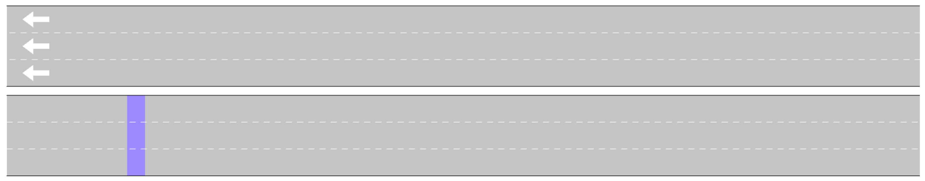
4.4. 0-Intersections
The model in
Figure 6 depicts a motorway environment with no intersections or traffic signals, implying that the traffic is uninterrupted and the only way to cause delays is to significantly increase the number of cars attempting to enter the network. This model was created to assess the difference of the adaptive approach on a motorway to that in an urban area with intersections. It features three lanes in each direction, with the innermost lane in each direction acting as a buffer lane for one direction of traffic at a time. This is the only feasible workaround to implement buffer lanes in Aimsun Next.
The traffic in this section traverses in a west–east or an east–west direction. The detectors are placed 10 m after the start of a street segment in each direction (the purple line in
Figure 6). Other models, such as the one represented in [
2], were also explored, but in order to have comparable findings for models with and without intersections, the models’ schemas were kept as basic and identical as feasible.
4.5. 1-Intersections
The network model in
Figure 7 represents an urban environment with an interrupted traffic flow. It is similar to the 0-Intersection model, as it contains three lanes in both directions, with the innermost lane acting as a buffer lane for one direction of traffic at a time as well as an intersection with an arterial-road section, with two lanes in each direction of traffic. Each section is 482 m long: one kilometre minus the width of the junction, which is placed directly in the middle. Again, the detectors were placed 10 m after the beginning of each horizontal section. It was later discovered that the distance between the detectors and the traffic lights influences how well the algorithms perform in this model. This will be discussed in
Section 7.3.
4.6. 2-Intersections
The significant difference from
Figure 8 to the 1-Intersection model is that there are two intersections evenly spaced along a road of one kilometre (310 m for each section). Each junction features two arterial roads with two lanes in each direction, as in the 1-Intersection model. The detectors were placed 10 m after the start of each horizontal section. However, unlike the 1-Intersection model, moving the detectors closer to the traffic signals had no discernible benefit.
4.7. Demands
Traffic demands can be represented as an origin–destination matrix in Aimsun Next, which defines how many cars travel from each origin to each destination on an hourly basis. In order to create traffic congestion, the capacity of a road section was manually determined, by evaluating various increased traffic demands. The road capacity, then, was periodically exceeded, as it is normal during rush hours in cities (see
Table 1 for the amount of vehicles to exceed the capacity of the roads). Minor flow refers to typical traffic flow that does not exceed the capacity of the road segment, whereas major flow refers to rush-hour traffic that exceeds the capacity of the road section. The terms upper and lower will be used to address the two ways in which the buffer lane might shift. The upper one represents the traffic direction of the primary street segment from east to west, while the bottom one represents the traffic direction from west to east (see
Figure 6).
A rush hours will always start with more traffic in the upper section, followed by the next rush hour in the lower section, and so on. The beginning and ending timings of rush hours for each demand may be found in
Table 2. The difference in the simulated minor and major flow between the 0-Intersection model and the other models is due to the traffic characteristics in those models. The motorway setting provides for uninterrupted traffic flow, whereas the urban setting is an interrupted traffic flow. Both types of models have been pushed to the point that a virtual queue, as part of the simulation in Aimsun Next, has formed outside of the simulated network, causing traffic congestion. This virtual queue is intended (see
Section 6 for a rationale).
- Demand 1
reflects a normal workday, covering 10 h, with major rush hours in the morning and evening, and two shorter rush hours in between. This was set up, as the algorithms were designed to primarily enhance travel times during daily commuting.
- Demand 2
is a compressed version of Demand 1, as it no longer simulates a regular workday and instead seeks to stress test the algorithms over the period of four hours, with repeated rush hours in opposing directions. This is done to emphasise the advantages of an adaptable approach in the face of rapidly changing traffic demands.
- Demand 3
adds one rush hour to Demand 2 because adaptive-lane reversal should yield greater efficiency, with more directional shifts than the static one, for example.
4.8. Static
A static-reversal schedule was established for subsequent comparison, which misses part of the rush hours, demonstrating the static-reversal management’s shortcomings. The reversal times for Demand 1 are as follows: the upper half uses the buffer lane from 0:00–7:00, while the lower half uses the buffer lane from 7:00–10:00, clearly missing two rush hours, which represent shorter rush hours but are not periodic in the training dataset. As these rush hours are not periodic, the static-traffic-control method cannot handle them. For Demand 2 and 3, the reversal times are as follows: the upper section uses the buffer lane from 0:00 to 3:00, while the bottom section uses the buffer lane from 3:00 to 4:00, or rather 5:00, in the case of Demand 3. Again, some rush hours will be missed.
4.9. False Negatives
False negatives in this work indicate that the algorithm will initiate a reversal, even if there is no rush hour in the now-reversed direction. This can occur when there is a brief increase in traffic in one direction that lasts just for the duration of the aggregation time period and then fades. The traffic demands do not reflect false negatives, as they would have minimal influence on the results, since the buffer lane can only be positioned in one of two directions. S false negative shifts the lane away from the direction that will be under rush-hour conditions next, forcing the algorithm to shift the lane again, but this already occurs in the models because the rush hours are always in the opposite direction of the current buffer-lane direction. Alternatively, the false negative leads the buffer lane to point in the direction of the next rush hour, which even improves network performance.
A significant number of false negatives in rapid succession may decrease the overall network performance, since the buffer lane is continually blocked for a given time period, due to the transition time, leaving it unavailable in both directions. However, this may be fine-tuned using the aggregation time frame. During the evaluation phase, it was discovered that the algorithm reversed too frequently, resulting in little performance loss, and it was decided that as a result, false negatives are not relevant enough to be considered.
5. Client-Server Architecture
The lane-reversal algorithm is implemented as a client-server application, and the code can only be made available for academic research. For this, the Aimsun Next model is provided with an application programming interface (API) module, written in Python 3, which acts as the client side (see
Figure 9). The API module is used to receive network calls in this case. The client sends relevant data to a Java server, where the data are processed and assessed as well as decisions are made. Since the client and server will communicate via rest endpoints, it is possible to replace either of them while maintaining a viable program, as long as all of the endpoints stay the same. This allows for the programming language to be changed in the future and makes it possible to integrate it into the Organic Traffic-Control System (OTC). This traffic-management system proposes an Observer/Controller approach that optimises intersection signalization and a self-organizing coordination mechanism that enables the design of traffic-responsive progressive signal systems (“green waves”) [
16].
5.1. Client
The initial client-side code was generated using the quicktype code generator [
17], which takes specifications in a JSON file to create classes in a wide range of languages. The resulting client-side code then was populated with logic that interacts with the servers’ rest endpoints. The client implements the 13 high-level Aimsun Next API functions (see
Figure 10), but only
AAPIInit,
AAPIManage, and
AAPIFinish are used. The induction-loop-detector characteristics are sent to the server-side in
AAPIInit at the start of the simulation. This message also informs the server that a new simulation has begun.
Since the buffer lane has to be attributed to one direction of traffic, AAPIManage performs the first policy activation at time step 0.0, assigning the buffer lane to the lower direction of traffic in this work. Since the initial rush hour always occurs in the top part, the algorithms are forced to reverse the buffer lane. This was done to ensure that the algorithms receive no unintended benefits. However, it is irrelevant which direction the buffer lane is allocated to in the initial time step, as long as the direction is consistent throughout all test cases. Since AAPIInit is unable to handle policies owing to separation of concerns, AAPIManage is used to activate the first policy, instead of AAPIInit.
In addition to the current time and direction of the buffer lane, the following measurements are transferred to the server every 0.8 s (the Aimsun default) via AAPIManage: number of cars passing a detector, occupancy, speed, and current density, as measured by the detectors in the previous time step.
Following the data transfer, the client awaits a response from the server, containing the decision as to whether or not the buffer lane is supposed to be reversed. After this, the client side either reverses the buffer lane or does nothing, and the simulation proceeds as usual. Eventually, AAPIFinish informs the server about the ending of the simulation.
5.2. Server
Java 11 was chosen as the programming language, to simplify the future integration into the Organic Traffic-Control System [
16]. The Java server analyses the simulation data and makes real-time decisions about the reversal, based on a variety of variables, depending on which algorithm is utilised in the current simulation. It is responsible for the decision logic, while the client only passes the data through and potentially reverses the buffer lane.
7. Results
The findings obtained during the evaluation phase
Section 6 are provided here, together with the evaluation process, parameter combinations, and evaluation criteria. More than 1300 simulations were conducted and evaluated to arrive at these conclusions.
7.1. Base Cases
To assess the overall approaches, two cases must be compared: the ‘static base’, as described in
Section 4.8, with its static reversal timings was conducted for each model. In comparison, for the ‘no-strategy base’, the buffer lane was assigned to one of the directions during a simulation. This was done for each direction, to allow for a fair comparison, without having to completely remove the lane. Otherwise, introducing a lane would obviously result in better travel times.
7.2. Turning Traffic
At least for the models shown in this work, the algorithms ceased to work as the amount of left-turning traffic increased too much: Potentially more cars will remain in the turning lane and block the buffer lane, which prevents or delays reversals. Furthermore, all algorithms rely on precise detector readings, but as the queue in the left lane grows, cars will come to a halt on the induction loop, rendering the acquired data useless.
More than 7.5% of left-turning traffic during the rush-hour phase resulted in significantly longer waiting times, until the reversal was completed. Once 15% left-turning traffic was achieved, the models failed totally because both ways were congested the whole time after the first few rush hours. This was due to a lack of space for left-turning traffic to relocate to, after a reversal commenced, as well as the detectors being occupied the entire time, due to the long line of turning vehicles.
This effect even occurred when there is no right-turning traffic. A possible solution for future work could be contraflow left-turn lanes, which allow for more free flow of left-turning traffic [
18]. As a result, it is advised to either limit the amount of left-turning traffic to a maximum of 10% or restrict it entirely.
7.3. Detector Placement
The distance between the detectors and the traffic lights affects how well each algorithm performs: the optimal for each method, however, was not identified in this work, since this would need significantly more experiments. For the 1-Intersection model, distances of 370 m and 470 m from the traffic light were tested to confirm the assumption that detector placement is more important for some algorithms than others. Generally, by moving the detector further away by 100 m, the ratio algorithm saw an improvement of up to 78%, while all the other algorithms performed worse, by up to 13%.
Based on this, the detectors should not be placed too close to the traffic lights. Cars stopping on the detector potentially trigger a reversal, even if the road segment is not congested. It is recommended that the appropriate distance is calculated by assessing the usual queue length at the traffic signal and then adding a few metres for safety.
7.4. Aggregation Time
While the 5 min aggregation time performed the best in all simulations, it was discovered to cause more reversals than the other aggregation times, perhaps contributing to driver confusion. It is better to choose a higher aggregation time based on the average length of a rush hour in the area, sacrificing some performance for the safety of all traffic participants. In the actual world, there may be false negatives, which are unlikely to be extremely long, since otherwise they would be considered actual rush hours.
7.5. Transition Time
When comparing the dynamic and fixed transition times for the 1-Intersection and 2-Intersection models, the dynamic-reversal-transition time, which waits for all vehicles to leave the buffer lane, performed best in most situations. It is also the safest option, as the entire lane in both directions is clear. Some of the static transition periods suffered performance losses when transitioning to the dynamic transition time. This suggests that the buffer lane was reversed while cars were still in the lane. This is unsafe in any situation.
If buffer-lane-clearance technology is not practicable and/or specific safety precautions are in place, static transition periods may be used in real-life situations. Instead of one traffic-signal cycle, the static transition time should then be based on two traffic-signal cycles, as this is the safer option.
7.6. Flattening
The flattening approach from the third evaluation phase only improved the performance of the flow-density algorithm, while all the other algorithms were unaffected.
7.7. Ratio Algorithm
The ratio algorithm beats any other algorithm presented in this work; with the proper parameter settings, this results in the algorithm regularly triggering up to 30 reversals on a four-rush-hour model. It is so sensitive that it can identify rush hours sooner than any other algorithm, but it will also trigger reversals when there is little to no traffic at all. As stated in
Section 6, the number of reversals must be kept to a minimum. Therefore, the parameter sets for the ratio algorithm were restricted to sets that resulted in an amount of reversals not more than twice the number of rush hours in the given model. With this constraints in place, the ratio method produced results equivalent to, if not outperforming, the other algorithms, at least on the 0-Intersection model. In the other scenarios, the ratio method consistently outperforms all other algorithms for Demands 2 and 3, while falling short for Demand 1 (the 10 h workday). This suggests a better performance, in case of quick reversals, that results in calm traffic rather than long periods of traffic surges.
However, due to the nature of the data acquired via induction loops, the ratio method has a severe flaw, making it the worst for Demand 1. Since vehicles travelling through the induction loop are counted, the number of vehicles passing through the induction loop falls when there is a traffic jam. This means that when fewer vehicles travel through the induction loop on a congested road, the ratio decreases. In other words, the buffer lane might be ‘reversed away’ from a busy road since it is no longer over the critical value.
Furthermore, in the 1-Intersection and 2-Intersection models, the ratio algorithm was the most sensitive to transition and aggregation times: In an urban traffic scenario, a little change might result in big performance increases but potentially massive performance losses. This implies a large effort in fine-tuning this algorithm to the specific location where it is being implemented. It was also established that detector positions have a substantial impact on this algorithm. Therefore, it might not be deployable at all street sections.
All of these points render this algorithm unsuitable for adaptive-lane reversal in urban areas.
7.8. Speed Algorithm
The speed algorithm failed completely on the uninterrupted-traffic model because the change in overall speed was not significant enough, making it unsuitable for such traffic situations. However, it performed well on the 1-Intersection and 2-Intersection models, almost always being second-best after the occupancy algorithm.
This algorithm, however, is quite sensitive to the critical value chosen. A change in value commonly causes additional reversals and dramatic variations in travel time.
7.9. Flow-Density Algorithm
With the exception of the aggregation time frame and transition time, which other algorithms must also deal with, there is no need to modify any critical value with this algorithm because it is calculated using a formula. This algorithm can be easily implemented in many locations with minimal adjustments. Regarding the aggregation time frame and the transition time, the algorithm is also highly robust: any changes cause only small fluctuations in the results. The most notable advantage of this approach is its improvability by flattening. This shrinks the gap between the best-performing algorithm while keeping its robustness.
However, the flattening approach, along with the 5 min aggregation time period, resulted in more reversals, while still being inferior to the occupancy algorithm.
7.10. Occupancy Algorithm
This algorithm performed the best in practically all of the examined cases (excluding the ratio algorithm), but only if very low values were used, which might lead to it being susceptible to false negatives. However, there is some leeway in adjusting the algorithm parameters and still having it be the best-performing algorithm. This algorithm also resulted in an almost ideal number of reversals in proportion to the rush hours.
Choosing a lower aggregation time frame nearly always had a positive effect, most commonly in the range of 1% to 13%, with each step. The algorithm gains more from a lower aggregation time, whereas the flow density, for example, only exhibits minor effects with the same steps.
7.11. Overall Results
All presented algorithms improved the performance of the travel time which can be seen in
Figure 11,
Figure 12 and
Figure 13. For the final evaluation, the occupancy algorithm will be used in comparison to the base cases, since it was consistently the best-performing algorithm: it resulted in an almost ideal number of reversals in proportion to the number of rush hours. The occupancy algorithm also performed better for Demand 1, which represents a normal working day. The final improvements obtained by the occupancy algorithm, in comparison to the base cases, are outlined in
Table 3, together with a conclusion of the results in
Section 8.
There is no mechanism to simulate driver urgency in Aimsun Next, making it difficult to compel all cars to exit the buffer lane right after a reversal. Even if the lane is closed for vehicles, according to an Aimsun policy, cars will remain in the lane and complete their intended current turn, despite the fact that other turning possibilities are available. In a real-world scenario, all of the results provided may be better, since human drivers might feel a sense of urgency when the buffer lane is about to reverse.
By setting the simulated cooperation level to 100%, this shortcoming was partly compensated for: other cars always let turning vehicles enter their lane without being selfish, but as certain cars have no desire to leave the lane, this does not solve the problem entirely.
8. Conclusions
Traffic congestion is a serious problem everywhere around the world. The alleviation of congestion would lead to a reduction in commuting stress, saving money and increasing productivity [
19]. To address this, four different tidal-flow-management algorithms were developed and evaluated using the traffic-simulation software Aimsun Next.
Three network situations were constructed to evaluate the performance of the algorithms: an extra lane for the upper direction, an additional lane for the lower direction, and a static approach. The total travel time, which includes waiting time outside of the network and driving time inside the network, as well as the number of reversals, was taken into account for the evaluation. To fine-tune the algorithm’s performance, three parameters were used: critical value, transition time, and aggregation time. The placement of a detector was identified as the fourth parameter. However, the potential of each algorithm having a perfect location was just noted and not investigated further.
Finally, after determining the best possible parameter combinations for each algorithm, the occupancy algorithm was identified as the best with regard to the criteria (travel time and number reversals), regardless of the fact that all algorithms improved travel time. Using the occupancy algorithm as the evaluation algorithm and depending on the compared base case, total travel time may be reduced in the 0-Intersection model by 0–81%, in the 1-Intersection model by 35–71%, and in the 2-Intersection model by 20–68%. With each additional simulated rush hour, the algorithms’ performance compared to the base cases increased.
8.1. Limitations
Although the algorithm performs well in a simulation, there are concerns regarding practical field implementation: an algorithm that repeatedly reverts the buffer lane, as the ratio method does, may cause driver confusion and impair the efficacy of the suggested solution. However, this issue could be mitigated by adjusting the aggregate timeframe as well as the transition time.
As previously noted, a longer aggregation period may result in minor performance losses of the suggested algorithms, which will, in turn, prevent the algorithms from triggering frequent oscillations. The transition time has little influence on total trip-time improvements and may, as indicated in this work, be changed within a reasonable range. A longer transition period will benefit traffic participants’ safety, since the danger of perplexing drivers will be minimised if adequate time is allowed for them to assess the new scenario.
These adjustments must all be taken into account during field implementation, which is why we have provided lower and upper constraints for algorithm improvements. We also created demand 2 and demand 3 to test how the algorithms react in case of frequent traffic directional changes. Since the safety of all traffic participants is essential, it is preferable to utilise the highest acceptable values for the aggregate timeframe as well as the transition time.
8.2. Future Work
Future plans include integrating the concept of adaptive-lane reversal in the Organic Traffic-Control (OTC) system—a self-adaptive and self-organised urban-traffic-management system that controls the green duration of traffic lights [
20], establishes progressive signal systems [
16] (“green waves”) and guides road users through the network using variable message signs [
21]. Possible challenges include devising a full decentralised extension of flow-lane reversal as well as using the OTC’s ability to adapt its control strategy for the improvements of such an extension.
Potentially, the results from this paper could be improved with some adjustments to the algorithms and the models chosen. Some of the improvements are described below.
8.2.1. Simulation Models
The models used in this work were as compact as possible, but larger models as well as real-life location models with real-life traffic data are required, to further investigate the influence of tidal-flow lanes in urban contexts. In this work, only five lanes in total were modelled. This number could be expanded to six or seven lanes, resulting in an algorithm that could reverse not one but several buffer lanes in each direction.
8.2.2. Algorithms
Ensemble techniques could be applied to combine the algorithms and mitigate their individual flaws. It could also be possible to learn the best set of parameters for each road segment automatically and individually. An algorithm that can decide on the reversal of several separate tidal-flow lanes that may interact with each other might be created to improve overall network performance.
8.2.3. Others
Additional studies in the field of reversible lanes could be conducted, as this work primarily focused on the everyday commute and associated traffic congestion. In addition, with usage of larger models, left turns and potential restrictions could be investigated. Furthermore, employing the algorithm from this paper, the topic of exclusive lanes, especially exclusive bus lanes, might be researched.
The premise of this work was that reversible lanes would be beneficial. Based on this, an additional procedure could prove for a given traffic flow that one party may receive higher benefits from a reversible lane than another.


