Article

Forecasting Survival Rates in Metastatic Colorectal Cancer Patients Undergoing Bevacizumab-Based Chemotherapy: A Machine Learning Approach

1
Department of Computer Science, Multimedia and Telecommunication, Universitat Oberta de Catalunya, 08018 Barcelona, Spain
2
Stanford Deep Data Research Computing Center, Department of Genetics, Stanford University School of Medicine, Stanford, CA 94305, USA
3
Research Center on Production Management and Engineering, Universitat Politècnica de València, 03801 Alcoy, Spain
4
Department of Telecommunications & Systems Engineering, Universitat Autònoma de Barcelona, 08202 Sabadell, Spain
*
Author to whom correspondence should be addressed.
BioMedInformatics 2024, 4(1), 733-753; https://doi.org/10.3390/biomedinformatics4010041
Submission received: 25 January 2024 / Revised: 20 February 2024 / Accepted: 29 February 2024 / Published: 2 March 2024
(This article belongs to the Special Issue Feature Papers in Computational Biology and Medicine)

Abstract

:
Background: Antibiotics can play a pivotal role in the treatment of colorectal cancer (CRC) at various stages of the disease, both directly and indirectly. Identifying novel patterns of antibiotic effects or responses in CRC within extensive medical data poses a significant challenge that can be addressed through algorithmic approaches. Machine Learning (ML) emerges as a promising solution for predicting clinical outcomes using clinical and heterogeneous cancer data. In the pursuit of our objective, we employed ML techniques for predicting CRC mortality and antibiotic influence. Methods: We utilized a dataset to examine the accuracy of death prediction in metastatic colorectal cancer. In addition, we analyzed the association between antibiotic exposure and mortality in metastatic colorectal cancer. The dataset comprised 147 patients, nineteen independent variables, and one dependent variable. Our analysis involved testing different classification-supervised ML, including an oversampling pool for classification models, Logistic Regression, Decision Trees, Naive Bayes, Support Vector Machine, Random Forest, XGBboost Classifier, a consensus of all models, and a consensus of top models (meta models). Results: The consensus of the top models’ classifier exhibited the highest accuracy among the algorithms tested (93%). This model met the standards for good accuracy, surpassing the 90% threshold considered useful in ML applications. Consistent with the accuracy results, other metrics are also good, including precision (0.96), recall (0.93), F-Beta (0.94), and AUC (0.93). Hazard ratio analysis suggests that there is no discernible difference between patients who received antibiotics and those who did not. Conclusions: Our modelling approach provides an alternative for analyzing and predicting the relationship between antibiotics and mortality in metastatic colorectal cancer patients treated with bevacizumab, complementing classic statistical methods. This methodology lays the groundwork for future use of datasets in cancer treatment research and highlights the advantages of meta models.

1. Introduction

Colorectal cancer (CRC) ranks as the third most prevalent cancer globally [1]. The development of CRC is associated with various risk factors [2,3]. Despite advancements in screening techniques and adjuvant therapy, metastasis remains the leading cause of death in CRC patients [4]. Approximately 50 percent of individuals diagnosed with colorectal cancer will eventually experience metastasis. Therapeutic interventions, such as chemotherapy, not only contribute to increased survival rates but also help alleviate symptoms in metastatic CRC (mCRC) patients [5]. In recent years, multiple studies have suggested a significant link between an imbalanced intestinal microbiome and the development of CRC. Microbial dysbiosis in the gut contributes to both the initiation and progression of CRC. Certain microbiota can promote carcinogenesis by producing carcinogenic toxins that manipulate inflammatory and tolerogenic pathways. The use of antibiotics has the potential to disrupt the normal microbiome, leading to an event known as dysbiosis. Indeed, various antibiotics have been shown to exert diverse effects on the density and diversity of the gut microbiota [6,7]. However, the gut microbiota can play dual roles, ranging from promoting tumorigenicity to exhibiting antitumorigenic effects. Manipulating the gut microbiota with antibiotics has shown promise in reducing tumour mass in mouse models of colon cancer. Moreover, previous studies have demonstrated that early exposure to antibiotics has significantly prevented tumorigenesis in a mouse model of inflammatory CRC. This approach holds practical therapeutic potential in managing CRC [8]. In a retrospective study involving 120 CRC patients, antibiotic treatment two weeks before commencing oxaliplatin-based therapy resulted in a significantly improved objective response rate (ORR) and disease control rate for progressive CRC. Additionally, in CRC patients, overall survival (OS) and progression-free survival (PFS) were notably higher in the group that received antibiotics [9,10].
Cancer analysis relies heavily on managing vast and variable datasets. However, there are many challenges that arise due to this data deluge, including noise, heterogeneity, sparseness, incomplete data fields, random errors, systematic biases, and the difficulty of extracting relevant clinical phenotypes. These challenges are partly generated by pharmaceutical and healthcare processes [11,12]. These complex data types come from diverse sources, including patient populations, environmental factors, medical procedures, and treatment protocols across different medical centers. The pathogenesis of CRC involves multiple factors, such as histopathology, genetics, and environmental factors. The intricate nature of this disease highlights the need for advanced and intelligent models, methodologies, and technologies to assist healthcare professionals in effectively combating it. Indeed, in order to navigate the complexities, uncertainties, and heterogeneity of today’s cancer landscape, it is crucial to employ agile, efficient, and intelligent solutions [13]. The application of Artificial Intelligence (AI) has the potential to enhance our understanding of various complex disease processes, enable personalized treatments, and optimize resources for individual patients.
Machine Learning (ML) models have demonstrated their effectiveness in predicting various clinical outcomes, such as acute renal damage, cardiovascular risk, and fracture risk, yielding promising results [14,15,16]. ML techniques have the potential to overcome the limitations associated with traditional statistical methods in risk prediction. These techniques can capture complex multidimensional relationships between features and clinical outcomes by leveraging algorithms to analyze extensive and diverse datasets [17]. ML approaches for cancer treatment are typically grounded in classification methods [18]. Many examples highlight the potential of ML in healthcare. For instance, classification methods have achieved a high accuracy in cancerous blood cell diagnostics for normal cells without the operator’s intervention in cell feature determination [19] or in dramatic situations like COVID-19 where deep learning methods, such as cutting-edge methods, have a significant tangible capacity for providing an accurate and efficient intelligent system for detecting and estimating the severity of COVID-19 [20]. And it can even be used for image analysis when analyzing brain Magnetic Resonance Imaging (MRI) data as a valuable, easier, and faster method for supporting healthcare professionals in examining MR images of newborn brains [21].
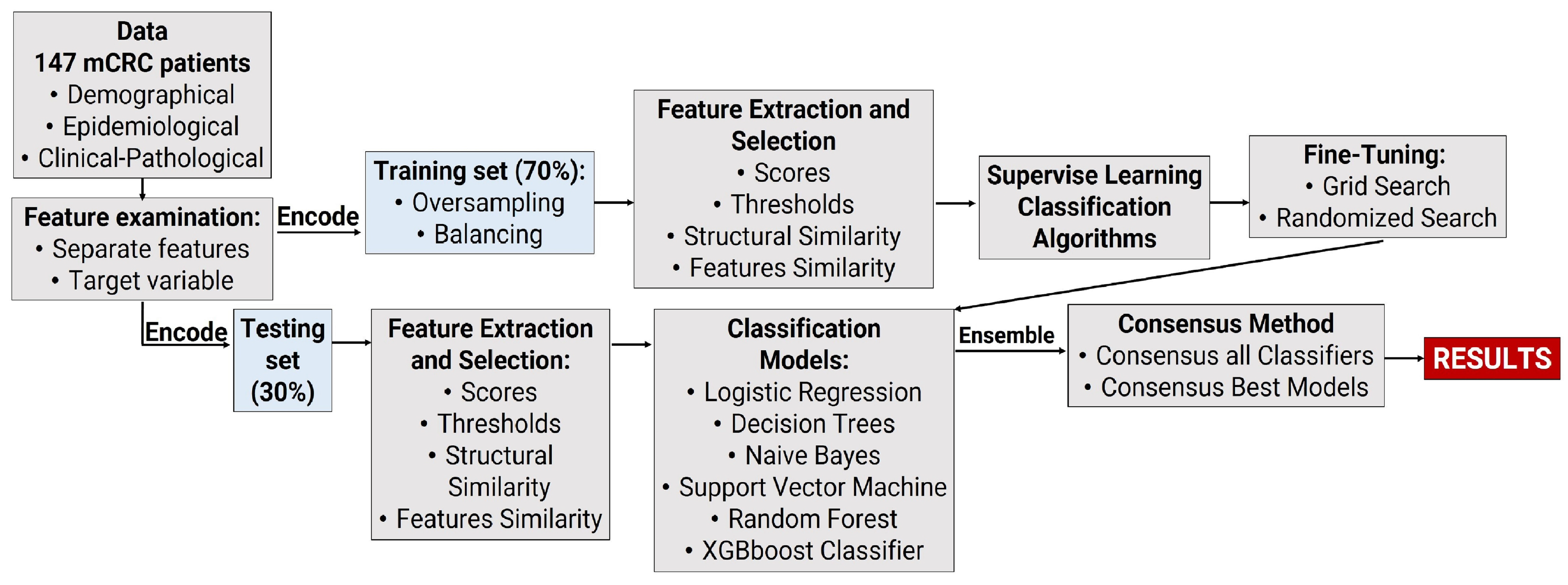
Classification methods are ML processes that group a set of input data into categories based on one or more variables. To achieve this, the model is trained with the training data and then tested with the test data before being deployed to make predictions on new data. Recent advancements in this field have introduced successful techniques like meta models. Meta models use the meta-learning methodology to learn the most appropriate algorithms and parameters for a particular ML task. These models aim to minimize the number of false positives and false negatives without compromising accuracy. The consensus learning approach is a variation of the ensemble methods that can be used to create multiple models and combine them to produce the best possible results. This technique is useful in improving predictability and reducing the variance within stochastic learning algorithms [22]. Ensemble methods differ from bagging (which combines many unstable predictors to create a stable ensemble predictor) and boosting (which combines many weak but stable predictors to create a strong ensemble predictor). It focuses on the use of a heterogeneous set of algorithms to capture even remote or weak similarities between the predicted sample and the training data [23].
The main objectives of this research are as follows: (i) develop predictive models that can forecast mortality in mCRC by using diverse data, including clinical and demographic information; (ii) create predictive meta-classification models that outperform supervised classification methods; (iii) construct predictive models utilizing clinical and demographic data to predict the connection between antibiotic medication and clinical outcomes in mCRC patients undergoing bevacizumab therapy, using the dataset from [24]; (iv) use ML methods to investigate potential correlations between the therapeutic outcomes of bevacizumab and various factors, including antibiotics, within the context of colorectal cancer and mortality; and (v) evaluate the potential of ML methods as an alternative for predicting the association between antibiotic medication and clinical outcomes in mCRC patients undergoing bevacizumab therapy in comparison to traditional statistical methods.
The rest of this paper is divided into different sections. In Section 2, the materials and methods used for the research are outlined. Section 3 describes the results obtained, followed by a comprehensive discussion in Section 4. Finally, Section 5 presents the research conclusions and discusses potential directions of future studies.
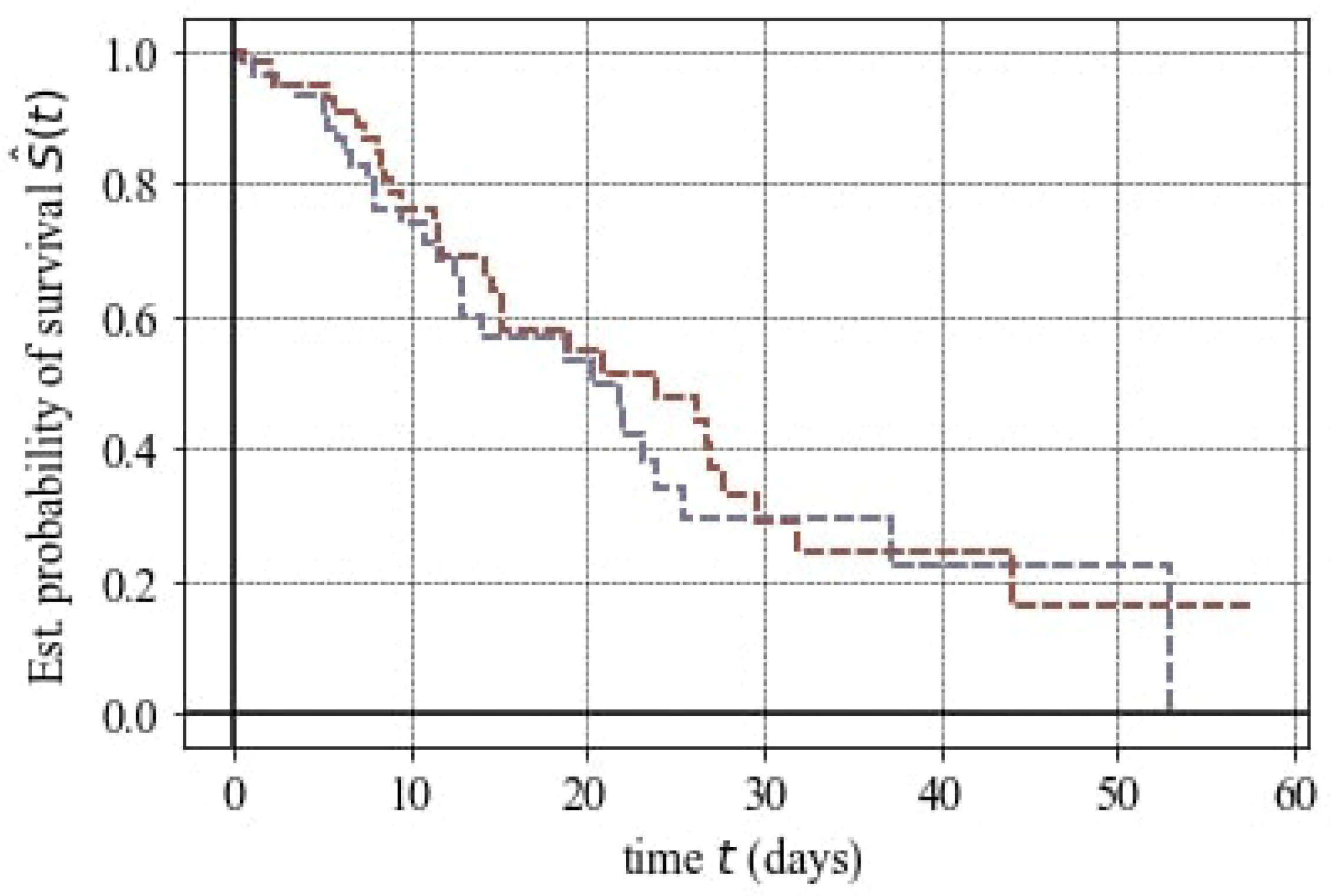
2. Materials and Methods

2.1. Sources of Data

A comprehensive search was conducted to find relevant research articles with clinical data on colorectal patients and information on antibiotic exposure during treatment. The search included databases like Scopus and MEDLINE, with a specific focus on open and freely accessible articles. The hospital-based retrospective cohort study conducted by [24] provided open-access data that were utilized. The dataset contains information from 147 mCRC patients, covering 18 independent variables and 1 dependent variable. These variables include demographic details, medical history, drug prescriptions, and disease outcomes. The specific variables used from this dataset are outlined in Table 1, and the workflow process used in the research is depicted in Figure 1. Although the type of antibiotic administered may have an impact, the dataset from [24] does not specify the antibiotic used. All pertinent data from the hospital-based retrospective cohort study conducted by [24] have been uploaded to Dryad at the following DOI: https://doi.org/10.5061/dryad.ft5sk66 (accessed on 11 December 2019).

2.2. Data Processing

All predictors consist of baseline characteristic data. The primary predicted outcome was mortality, while the remaining variables were considered secondary outcomes. For the outcome variable, Class 0 denoted the non-occurrence of the event, while Class 1 indicated the occurrence of a categorical effect. To address incomplete datasets, three options were considered for proceeding with the analysis: (i) removing data (partial deletion), (ii) imputation (assigning missing values by inference), or (iii) retaining the missing values and employing a model that incorporates them. It is noteworthy that no missing data were observed. Thus, the dataset was separated into features and target variable (Death) and then further split into test and train datasets. A kernel density estimate (KDE) analysis was created to visualize the distribution of observations in both the train and test datasets. KDE represents the data through a continuous probability density curve in one or more dimensions. This method was employed to ensure comparability between the datasets [25].

2.3. Software

All analyses in this study were conducted using Python, a cross-platform, free, and open-source programming environment. Python was utilized for data manipulation, visualization, and ML model training. Python programming language version 3.10.12 [GCC 11.4.0] was used to perform the analysis, along with its comprehensive libraries for data management, statistical computing, and graphical visualization. Default parameters were employed for each programming function unless explicitly specified. Our analysis made use of various Python libraries, including NumPy (Version 1.25.2) [26], pandas (version 1.5.3) [27], Statsmodels (version 0.14.1) [28], Matplotlib (version 3.7.1) [29], Seaborn (version 0.13.1) [30], and scikit-learn (version 1.2.2) [31].

2.4. Model Development

Different classification models and meta-classification models were analyzed. Classification models were based on a pool of models, such as GaussianNB [32], LogisticRegression [33], RandomForestClassifier [34], DecisionTreeClassifier [35], XGBClassifier [36], and SVC [37]. Afterwards, two meta models were developed based on all classifiers and top models’ classifiers. Their development was based on stacking methods, which represent a strong ensemble learning strategy in ML that combines the predictions of numerous base models to obtain a final prediction with better performance. Meta models aim to minimize the number of false negatives and false positives without compromising accuracy. It is a way to recognize and draw conclusions from connections among data and balance the generality of the solution and the overall performance of the trained model. The selection of these models was purposeful, aimed at harnessing their individual strengths and complementarity. GaussianNB and Logistic Regression were chosen for their simplicity and efficiency in handling linear relationships, while Random Forest Classifier and Decision Tree Classifier were selected for their capacity to capture complex non-linear patterns in the data. XGBoost Classifier and SVC were employed due to their robustness in managing imbalanced datasets and high-dimensional feature spaces. Additionally, meta models were integrated to aggregate predictions from multiple base models, thereby enhancing overall performance and interoperability. Despite recognizing the limitations of our dataset, including its relatively small size and lack of external validation, we remain vigilant about the importance of employing a robust methodology to ensure the reliability of our findings. Moreover, we have taken proactive measures to address potential biases in the analysis to the best of our ability.
Categorical features were encoded as a one-hot numeric array using OneHotEncoder [38], oversampling and balancing to balance the dataset [39]. Then, it was ensured through consistent encoding merging or concatenating multiple DataFrames in Python, to make sure that the encoding (character encoding) of the resulting DataFrame was consistent. As a consequence, this function increases the number of observations in a balanced manner. The cohort was randomly split into the development cohort ( 70 % ) and the validation cohort ( 30 % ), following the classical split-sample internal-validation approach. The development cohort was used for training ML models and tuning their parameters, while the validation cohort evaluated the developed models’ performance on unseen data.
ML models often involve essential parameters that cannot be directly estimated from the data. To optimize performance, tuning parameters allow adjustments to be made to settings within an algorithm. Tuning hyperparameters involved systematically testing different model parameters to optimize the performance of the ML models based on GridSearchCV and RandomizedSearchCV methods. GridSearchCV is a method provided by Scikit-learn [40] that allows you to perform an exhaustive search over a specified parameter grid for an estimator. It helps you find the best combination of hyperparameters for a given model. This is especially useful when you want to tune the hyperparameters of your models to achieve better performance. On the other hand, RandomizedSearchCV is another hyperparameter optimization technique provided by Scikit-learn [40], similar to GridSearchCV, but instead of trying all possible combinations of hyperparameters, it samples a fixed number of hyperparameter combinations from specified probability distributions. This can be more efficient when the search space is large. Finally, the following models have been used: Oversampling pool for models (M1), Logistic Regression (M2), Decision Trees (M3), Naive Bayes (M4), Support Vector Machine (M5), Random Forest (M6), XGBboost Classifier (M7), Consensus all meta-model (M8), Consensus top meta-models (M9). Throughout the training phase, the optimal ML model assesses each feature and assigns it a weight, determining the strength of its contribution to predicting the target variable. The objective is to clarify the prediction of a target variable, denoted as Y (Death), by quantifying the contribution of each feature to that prediction [41].

2.5. Model Evaluation

The evaluation criteria for binary factors typically encompass accuracy, precision, recall, F-beta, and the area under the curve (AUC) [42]. While achieving high accuracy might demand 99 % , industry standards for satisfactory accuracy generally exceed 70 % [43,44]. The same range was considered for the other model evaluation metrics. Table A1 in Appendix A presents the confusion matrix, delineating four distinct outcomes. A confusion matrix is a table used to define a classification algorithm’s performance. It visualizes and summarizes the performance of a classification algorithm. These include true positives (TP), where the prediction accurately indicates death; false negatives (FN), where the prediction inaccurately suggests no death; true negatives (TN), where the prediction correctly indicates no death; and false positives, where the prediction erroneously indicates death.
Accuracy, recall, precision, and F-beta are calculated as described in Equations (A1)–(A8) in the Appendix A. Recall is a crucial evaluation metric utilized in classification and information retrieval tasks. It quantifies the proportion of true positive cases correctly identified by the model among all positive cases in the dataset. Conversely, accuracy, often referred to as precision, serves as a metric for assessing the correctness of a classification model. It measures the proportion of correct predictions, encompassing both true positives and true negatives, among all predictions made by the model. Both accuracy and recall should be as high as possible. However, these two factors are inversely related, necessitating a balance. Consequently, the F-beta was employed to reflect the comprehensive performance of the model. The recall is also called sensitivity or true positive rate (TPR). The classification report visualizer displays the precision, recall, F1, and support scores for the model. In addition, the metrics extracted from the confusion matrix, such as precision, recall, and beta-score for each class and micro, macro, and weighted average of all classes, are used for measuring the overall performance of a classifier. In addition, other metrics related to the confusion matrix were defined to support the value number of occurrences of each particular class in the true responses (test set). This was calculated by summing the rows of the confusion matrix. Macro average is the mean of the recalls of classes, positive or negative. Also, the sum of the scores of all classes after multiplying their respective class proportions is called weighted average [45].
When both accuracy and recall are equally important (beta = 1, F-1 score), they are given the same weight. However, in this study, type II errors, specifically situations where patients with abnormal blood concentrations were not assessed, were of particular importance due to their negative impact on treatment outcomes. Type II errors are generally measured by recall. Therefore, this study assigned greater weight to recall (beta = 2, F-2 score). The F-beta score ranged between 0 and 1, with a larger value indicating better model performance. Ultimately, the model is deemed meaningful when the area under the curve (AUC) exceeds 0.5 . AUC can be calculated using the formula in Equation (A6), where true positive rate (TPR) and false positive rate (FPR) are calculated using Equations (A7) and (A8) in Appendix A, respectively.
The model’s performance was assessed using the receiver operating characteristic (ROC) curve with Sklearn.metrics and roc_curve roc_auc_score [46]. The ROC curve is a valuable tool for visualizing and quantifying the discrimination ability of a binary classification model, while the area under the ROC curve (AUC) provides a summary measure of the model’s performance.

2.6. Feature Importance and Partial Dependence Plots

The importance of different features on the model outcome was calculated using the SHAP package. SHAP values (SHapley Additive exPlanations) leverage cooperative game theory to enhance the transparency and interpretability of machine learning models. This method unveils the individual contribution of each feature, akin to a player in a game, to the output of the model for each example or observation [47].

2.7. Risk Stratification Using ML

The death prediction task was approached as a binary classification problem, with machine learning models generating a probability of death risk ranging from 0 to 1. The risk probabilities calculated by the best-performing machine learning model were utilized to determine optimal cutoff values, effectively stratifying patients into two risk groups (low and high). This stratification was achieved by maximizing the F1 score. Following this, the survival probabilities of these risk groups were assessed using the Kaplan–Meier method [48].

3. Results

This section provides an overview of the results obtained, encompassing essential patient characteristics, model performance, feature analysis, predictions, and the validation and comparison of the developed models.

3.1. Descriptive Analysis

The association between antibiotic exposure and cancer mortality has been a longstanding focus in cancer research [49,50,51,52]. However, drawing reliable conclusions for such associations has faced many challenges. Adding to the complexity, clinical data for analysis are often not openly accessible due to intricate privacy and ethical policies restricting their usage. Moreover, these datasets are frequently both heterogeneous and extensive. Despite these challenges, our analysis leveraged 147 observations, covering 19 variables, to investigate mortality in CRC, as detailed in Table 2. Continuous variables are presented as the mean ± standard deviation, along with corresponding p-values obtained from the t-test. Categorical variables are expressed as percentages, with associated p-values derived from the Chi-squared test. Importantly, no significant differences were observed in the demographic, clinical, or epidemiological data between the training group ( N = 102 ) and the test group ( N = 45 ).
For instance, our analysis reveals that, on average, the age at the time of diagnosis is 68 for men and 72 for women. This aligns with the understanding that the majority of colorectal cancers occur in individuals older than 50. Notably, for colon cancer, the average age is 63 for both men and women, as reported in [53]. Although Table 2 presents the distribution of sexes between males and females and underscores the importance of sex in colorectal cancer (CRC), our research analysis did not stratify the sexes. While up to 50 % of colon cancers may have a strong inherited factor, it is important to note that diet and lifestyle play essential roles in rectal cancer. Excess weight is associated with an increased risk of cancer. However, it is not considered an essential factor in this population group [54,55]. Additional characteristics outlined in Table 2 underscore that metastasis remains the leading cause of cancer-related mortality in CRC patients, primarily due to the spread of cancer to other body parts [4,56]. This is particularly significant in rectal cancer, where the overall survival (OS) for individuals diagnosed at a localized stage is significantly higher compared to cases where cancer has spread to distant parts of the body [57]. Consequently, metastases contribute to over 40 % of cancer-related mortality in CRC patients. Cancer data analysis often reveals high variability and influence among cancer variables. The interpretation of treatment effects is significantly impacted by PFS, introducing subjective biases related to treatments [58]. The location of the colorectal tumor is a crucial factor in disease progression and overall survival [59]. Notably, patients undergoing radical surgery have a higher likelihood of receiving a metastasis diagnosis. Combining the Bevacizumab monoclonal antibody with chemotherapy has demonstrated greater efficacy than treatments involving only chemotherapy or the monoclonal antibody. However, this combination may also elevate the risk of some adverse gastrointestinal adverse [60].
When analyzing different variables, one should consider whether the observations are independent or not. This is particularly important when no repeated measure design or matched data exist. In this analysis, we found no repeated observations. We calculated the correlation coefficient and presented it in a heatmap to better understand the relationship between each pair of independent variables (Figure 2). Based on the assumption of independence, we have excluded the following independent continuous variables: Age, OS, Dosage, Antibiotic Days, Weight, and BMI. These variables showed a high correlation coefficient ( 0.5 ) with each other. Generally, a weak positive correlation falls between 0.1 and 0.3 , a moderate correlation between 0.3 and 0.5 , and a strong correlation between 0.5 and 1.0 [61].
Figure 3 presents a heatmap plot illustrating the correlation coefficients among all variables, including both continuous and categorical ones. Positive correlations are notably observed between BMI and Weight (WT), as well as between Antibiotics, Antibiotic Range, and Antibiotic Days, reflecting their inherent dependencies. The remaining correlation coefficients are approximately zero, signifying an absence of statistically significant correlations.
KDE analysis was conducted for all variables utilized in the models, demostrating the distribution of observations across both the training and testing datasets. The consistency observed in these plots implies no notable disparities between the training and testing datasets, affirming their comparability. Detailed information regarding the dataset split, ensuring balance, is provided in Table 2, obviating the need for graphical representation in the KDE analysis.

3.2. Model Performance

The confusion matrix in Figure 4, as well as the one associated with the classification report, shows the performance of the nine classification models. The figure provides a comprehensive comparison of the models based on the test data for the actual and predicted counts of each class, while a classification report shows the calculated metrics of each class. Similar results were observed among the various models considered in terms of accuracy, precision, recall, F-Beta, and AUC. Although these metrics may not reach the typically defined standards, they align with results seen in other clinical research [42,62].
The confusion matrix for the Consensus Top Meta Models identifies the types and sources of errors a model makes, while the classification report helps to evaluate the quality and reliability of the model. As a result, the Consensus Top Meta Models demonstrated superior performance in terms of various metrics when compared to the other models. Operating as both a statistical approach and an ML algorithm tailored for classification problems, M9 is founded on the probability concept. Notably, M9 possesses the ability to map any real value onto a scale within the range of 0 to 1. M9 relies on several fundamental assumptions to maintain its effectiveness. Consensus Top Meta Models refers to a set of meta models that have been widely accepted or agreed upon as the most prominent in a particular domain. These models, having achieved a consensus within the community or industry, represent distinguished and effective approaches to addressing specific challenges or issues in the corresponding field. This term underscores the convergence of opinions and recognition surrounding these meta models as leading benchmarks in their application area [63]. The M9 model has met the benchmarks that are indicative of a valuable ML model. While the requirement for high accuracy may vary based on the specific objectives of the model, industry standards generally deem an accuracy above 90% as satisfactory. Similar criteria apply to other metrics, with values approaching 100 % or 1 considered more favorable. Consequently, the meta model has emerged as the optimal classification model. Table 3 displays the obtained model parameters, encompassing the coefficient for each independent variable, accompanied by its coefficient standard error, z-value, p-value, and 0.025 and 95 % confidence intervals (CI). Importantly, it is observed that three of the independent variables, Treatment, Site, and Differentiation, present p-values exceeding 0.05 , indicating that they are not deemed statistically significant predictors. To enhance the reliability of the model, a subsequent Consensus Top Meta Model was conducted, excluding the non-significant variables. Notably, the antibiotic variable exhibited a p-value larger than 0.05 ( 0.159 ), exposing no significance association with mortality in metastatic colorectal cancer (mCRC) patients treated with bevacizumab.
The refined M9, optimized by excluding the Treatment, Site, and Differentiation variables, as mentioned earlier, was constructed. Despite the acknowledged impact of differentiation grade on survival time [64], it is worth noting that poorly differentiated CRCs often exhibit heightened aggressiveness and a lack of targeted therapies [65]. The parameters of the optimized model were derived from the variables detailed in Table 4. Notably, the optimized M9 model reveals that the antibiotic variable has a p-value > 0.05 . It is significant to observe that the p-value for antibiotic exposure is 0.182 . Therefore, previous assumption related to mCRC and antibiotics could be maintained. Nevertheless, several questions remain unanswered, including details about the specific type of antibiotic, dosage, or mode of administration (oral or intravenous), which could offer more nuanced conclusions. Furthermore, while the meta model demonstrated the highest prediction accuracy, there is still room for improvement to enhance both accuracy and precision.
Scrutinizing these assumptions unveils that M9 can be applied with greater flexibility than conventional regression procedures, rendering it suitable for various therapeutic circumstances. In any given scenario, M9 computes the probability that a case with a specific set of values for the independent variables belongs to the modelled category [33]. Consequently, M9 finds frequent application in health sciences studies, particularly in models concerning illness conditions (diseased or healthy) and decision making (yes or no). To improve prediction accuracy, the meta model was analyzed with consideration of the number of independent variables required, ensuring that accuracy was not compromised. The influence of each independent variable on the model’s accuracy was evaluated by iteratively running the model, excluding one variable at a time to measure the impact of its omission on accuracy. The results are presented in Table 5. The table illustrates the effect of omitting each independent classification variable on the model’s accuracy, utilizing the test dataset. Notably, Hypertension, Differentiation, ECOG, and Treatment had a substantial impact (≥3) on the accuracy, designating them as significant predictors.
Generally, an AUC of 0.5 suggests no discrimination, 0.7 to 0.8 is considered acceptable, 0.8 to 0.9 is deemed excellent, and values above 0.9 are considered outstanding. The M9 model exhibited an AUC of 0.93 (Figure 5), indicating an acceptable level of discrimination. Nevertheless, there is room for improvement to achieve a higher AUC.

3.3. Feature Analysis

Figure 6 illustrates the significance of each model’s features. Nearly all of the models demonstrated a consistent significance in the structural aspects of each model’s features. All models incorporated OS, Age, and PFS, underscoring the relevance of dietary and lifestyle factors in colorectal cancer (CRC) [54,55]. However, the positions of ECOG, BMI, and Antibiotic Days were permuted in various models, as were Metastasis Organs and PFS, along with Site, Surgery, Sex, and Antibiotics. Despite these variations, similar significance values were observed for each model’s features across the nine models. Even though the Antibiotic variable does not present a high significance, Antibiotic Days do. For this reason, taking a cancer treatment at the same time as an antibiotic could have a high influence on survival [52].

Clinical Significance

The survival function derived from the Kaplan–Meier estimator provides a valuable quantification of survival analysis, depicting the relationship between time and the probability of surviving beyond a specific time point. Figure 7 visually represents the probability of survival over time. At any given moment, the survival function is computed as the ratio of patients surviving beyond that point to the total number of patients. The resulting curve takes the form of a step function, with steps occurring at time points where one or more patients have died. The plot distinctly indicates that there is no apparent difference between patients who took antibiotics and those who did not.
The findings illustrated in Figure 7 were supported by the Hazard Ratio (HR) value. Hazard Ratios were employed in survival analysis to compare the risk of death between patients who took antibiotics and those who did not. The obtained HR value was one, signifying that as the HR covariate increases by 0 % , there is no significant difference in event hazard between different Antibiotic groups.

4. Discussion

Our study suggests that a range of ML models can proficiently predict and classify cancer-related issues. The top meta models identified by consensus exhibited superior performance across various metrics. These consensus models introduce a novel weighted method explicitly crafted to minimize false negatives and false positives while maintaining accuracy. In the proposed weighted consensus model, we normalize the accuracy of individual classification models. During the prediction phase, these models might predict different classes. In the experimental evaluation of the weighted consensus model, we utilized classification algorithms, including Logistic Regression, Decision Trees, Naive Bayes, Support Vector Machines, Random Forest, and XGBoost. Our results indicate that the proposed meta-model performs comparably to the current state-of-the-art techniques, achieving an accuracy of 93 % . Notably, it effectively mitigates false negatives and false positives. One noticeable application of the meta-model in our study involved examining the association between antibiotic exposure and clinical outcomes in mCRC patients. This analysis, reminiscent of a hospital-based cohort study, confirmed a non-significant association, aligning with the findings of other studies [24]. However, an important observation emerged—the duration of antibiotic exposure during cancer treatment holds more significance than the mere presence or absence of antibiotic use [52]. Our study underscores that the period of antibiotic treatment could exert a substantial influence on survival outcomes. This insight adds depth to our understanding, suggesting that assessing the duration of antibiotic use is crucial for a more nuanced interpretation of its impact on clinical outcomes. ML methods have shown promising features in cancer prediction, as evident in studies related to breast cancer and large-B-cell lymphoma (DLBCL) [66,67,68]. These methods contribute to informed decision making in clinical practice for colorectal cancer. However, challenges such as dataset size, quality, and algorithm selection persist. The dataset’s quality and the algorithm’s appropriateness depend on factors like data types, sample size, time constraints, and desired prediction outcomes. Overall, the successful performance of the meta model suggests that they could be valuable tools in real-world clinical settings. By providing accurate predictions of cancer survival, these models can aid in individualized treatment strategies, optimizing dosage regimens, and ultimately improving therapeutic outcomes.
Antibiotics play a pivotal role in the management of colon cancer (CRC) across various disease stages, exerting both direct and indirect effects. However, their efficacy can vary based on the specific type utilized. Emerging research indicates that different antibiotic classes may elicit varied responses in certain cancers, potentially impeding tumour growth. Conversely, the effectiveness of previously administered antibiotics may diminish over time. Despite being commonly employed as adjuvant therapies alongside surgical, radiotherapeutic, chemotherapeutic, and immunotherapeutic interventions, concerns regarding antibiotic resistance and reproductive toxicity are mounting. Moreover, antibiotic usage can disrupt the balance of the intestinal microbiota, thus affecting the efficacy of combined cancer treatments [69]. Consequently, careful consideration must be given to selecting the optimal type, dosage, and administration route (oral or intravenous) of antibiotics to synergize with cancer therapies.
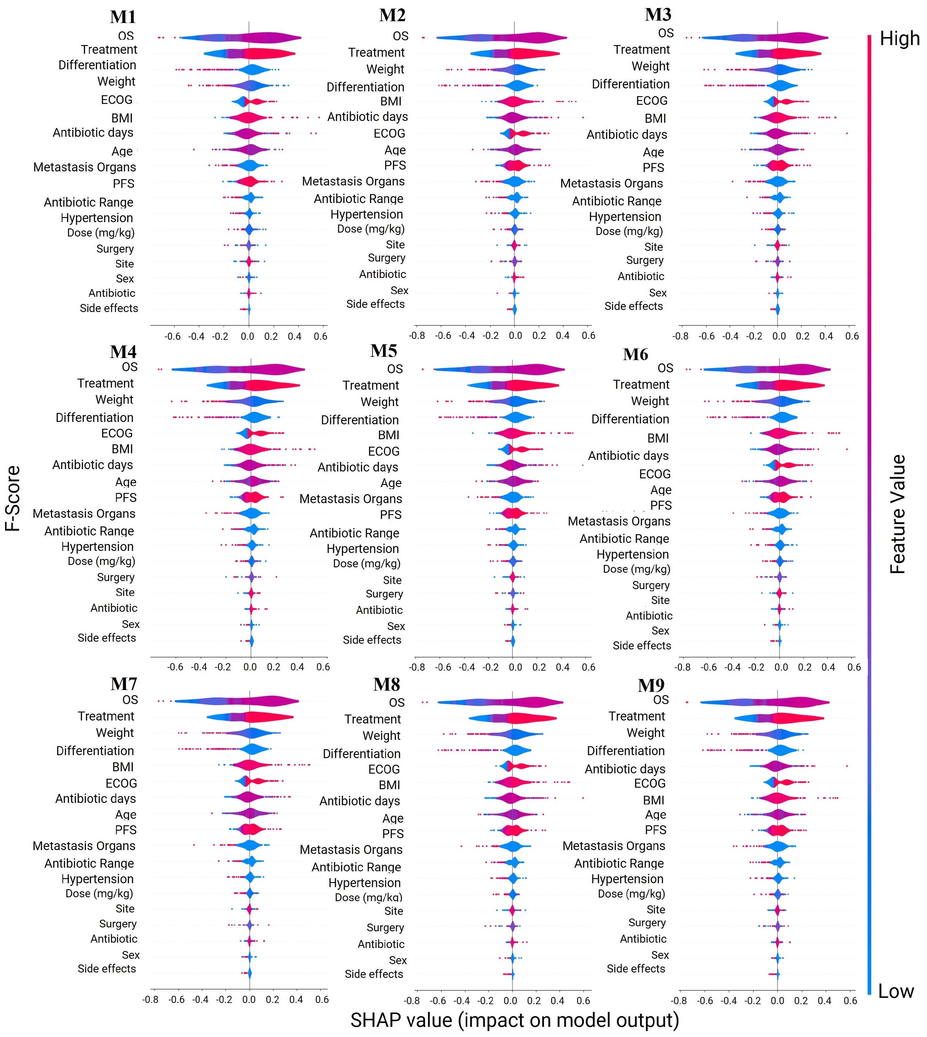
The feature importance analysis for the classification models has uncovered that certain antibiotic-related variables are more influential than the mere presence or absence of antibiotic use. This discovery aligns with the existing knowledge in the field, where the impact of antibiotics on cancer survival lacks clear significance. Our results expand on this understanding by evaluating the importance of the specific type of antibiotic used in cancer treatment. Indeed, different antibiotics have been shown to exert varying effects on the density and diversity of the microbiota [6,7]. This nuanced insight contributes to the ongoing discourse on the role of antibiotics in cancer treatment, highlighting the need for a more comprehensive consideration of the various factors at play.
While colorectal cancer can affect individuals of all genders, current evidence does not indicate a differential impact of gender on the incidence of colon cancer itself [70]. However, certain risk factors, such as the influence of sex hormones and age, may vary between genders and contribute to the development of colon cancer. Furthermore, variations in symptoms and clinical presentation have been observed between men and women diagnosed with colon cancer. Therefore, any analysis of colon cancer must take into account these gender-related factors. Consequently, future analyses should consider stratifying the data by sex to explore potential differences between females and males in colorectal cancer outcomes and the impact of antibiotics on their survival [71].
Unfortunately, different datasets present different variables, making it challenging to make comparisons between different studies. The analysis of cancer heavily relies on managing vast and variable datasets. Challenges arising from this data deluge include noise, heterogeneity, sparseness, incomplete data fields, random errors, systematic biases, and extracting relevant clinical phenotypes. All of these challenges are generated by pharmaceutical and healthcare processes [11,12]. Consequently, the comparable analysis makes it difficult to perform. For this reason, it is essential to acknowledge that these studies faced certain limitations. Firstly, they often dealt with a relatively limited amount of data, which may impact the generalizability of their models. Additionally, the lack of external validation in many of these studies raises concerns about the robustness and reliability of their findings. Finally, heterogeneity and not homogeneity between hospitals or research centres make it difficult to analyze the generalizability of the impact of these models. Even though a small-sample-size dataset may limit the ability to detect small size effects and can lead to overestimation or underestimation of size effects, our study relied solely on a small public dataset, which is a constraint of our research. While the dataset exhibits high accuracy, its generalizability is constrained by several limitations. These include its relatively small size and the lack of external validation. Recognizing and mitigating these limitations are crucial for a more precise interpretation of the findings. Additionally, it is essential to proactively address any potential biases in the analysis.
Working with larger and more diverse datasets, including private datasets, may lead to different or complementary findings, such as identifying other determining factors that can be significant in predicting the impact of bevacizumab in the treatment of mCRC patients. However, meta models can adaptively balance the effect of meta learning and task-specific learning within each task, minimizing the possibility of having imbalance and overfitting problems. In a published study, a meta-analysis on 2760 mCRC patients suggested that primary tumour resection was the critical factor in the improved survival of mCRC patients who received bevacizumab treatment [72]. A systemic review and meta-analysis of nearly 4000 previously untreated or advanced mCRC patients showed that the combination of chemotherapy and bevacizumab increased the survival rates of patients who had not received prior chemotherapy for metastatic colorectal cancer. The patients who received bolus 5-FU or capecitabine-based chemotherapy with bevacizumab showed higher progression-free survival and overall survival rates compared to those who received infusional 5-FU plus bevacizumab, where there was no difference in progression-free survival and overall survival [73]. In a study that examined the impact of primary tumour location on the efficacy of bevacizumab combined with CAPEOX (capecitabine and oxaliplatin) in the first-line treatment of metastatic colorectal cancer (mCRC), researchers found that patients with primary tumours in the sigmoid colon and rectum had significantly better outcomes in terms of progression-free survival (PFS) and OS compared to those with primary tumours from the cecum to the descending colon. This study included a cohort of 667 mCRC patients treated with CAPEOX and bevacizumab from 2006 to 2011, revealed a median PFS of 9.3 months and a median OS of 23.5 months for patients with sigmoid colon and rectal tumours, substantially better than the outcomes for patients with tumours in other locations. These findings were consistent even after adjusting for other prognostic factors in multivariate analyses. However, for patients treated solely with CAPEOX, no significant association between primary tumor location and treatment outcomes was observed. This suggests that the addition of bevacizumab to CAPEOX may predominantly benefit mCRC patients with primary tumors in the rectum and sigmoid colon, a hypothesis that warrants further validation through data from completed randomized trials [74]. These studies demonstrate that other factors, such as chemotherapy regimes, tumour resection, and primary tumour location, can change the outcome of using bevacizumab in mCRC patients. Thus, the impact and effectiveness of using this antibiotic in the treatment of mCRC patients cannot be predicted accurately without considering other factors that affect cancer pathophysiology as well as patients’ health and survival.

5. Conclusions

In this paper, we presented a weighted consensus model that achieves high accuracy in identifying potential mCRC-related deaths. We also investigated the impact of administrating an antibiotic, bevacizumab, on mCRC patients. To predict survival in mCRC, we employed machine learning classification algorithms. Our analysis was based on multi-source and heterogeneous clinical data obtained from openly accessible datasets. Our findings showed that the presence or absence of antibiotics did not have a significant predictive value for mCRC survival. However, upon closer examination, we found that the variable ‘Antibiotic Days’ was the most crucial predictor in our study. Our analyses suggest that an increase in ‘Antibiotic Days’ is positively correlated with cancer progression and mortality in mCRC patients, emphasizing the importance of not only considering the use of antibiotics but also paying attention to their duration. This phenomenon can be correlated to the cumulative bevacizumab dose (CBD) caused by increasing the ‘Antibiotic Days’ as it was reported in another study [75] considering the terminal half-life of bevacizumab is relatively long (about 20 days) in both men and women [76].
We used resampling techniques to overcome the limitations of the clinical data, such as data dependence and bias. Variables were screened based on their importance, and we compared the performance of ten different classification ML models. Although antibiotics had an impact on the study, they were not considered significant in terms of survival. Ultimately, we chose the logistic regression model as the best predictive model, with an accuracy of 93 % , indicating robust prediction capabilities across the clinical data. Our proposed consensus method is a novel technique that minimizes false negatives and false positives, depending on the requirements. This model has the potential to reduce the death of mCRC patients by minimizing false negatives and positives. In contrast, the rest of the classification methods exhibited an accuracy of 60 % to 87 % , suggesting that most of them were good predictors for this study, taking into account that industry standards for satisfactory accuracy generally exceed 70 % and can be up to 90 % [43,44].
Overall, our study sheds light on a potentially critical aspect of the intricate relationship between antibiotics and mCRC survival, offering valuable insights for future research and clinical considerations. This study further elaborates on the ability of ML to predict survival in mCRC. Our findings highlight the predictive potential of the implemented ML classification models in mCRC. While the capabilities of ML methods continue to enhance and more patient data become available to cancer researchers, future studies can uncover further details of associations between specific classes of antibiotics and chemotherapy regimens in mCRC treatment. Notably, future studies can analyze other datasets containing data such as antibiotics, mCRC, and survival, aiming to elucidate other possible significant relations.

Author Contributions

Conceptualization, S.S.-H., A.T., E.P.-B., A.A.J. and L.C.; methodology, S.S.-H., A.T. and L.C.; software, S.S.-H. and A.T.; validation, E.P.-B., A.A.J. and L.C.; writing—original draft preparation, S.S.-H. and A.T.; writing—review and editing, E.P.-B., A.A.J. and L.C.; supervision, E.P.-B., A.A.J. and L.C. All authors have read and agreed to the published version of the manuscript.

Funding

This research received no external funding.

Institutional Review Board Statement

Not applicable.

Informed Consent Statement

Not applicable.

Data Availability Statement

All data utilized in this study are publicly available.

Acknowledgments

We would like to express our gratitude to the authors whose references were utilized in this study, which aims to juxtapose our ML methodologies with real-world data from open publications.

Conflicts of Interest

The authors declare no conflicts of interest.

Abbreviations

The following abbreviations are used in this manuscript:
ABAdaBoost classifier
AIArtificial Intelligence
AUCArea under the curve
CRCColorectal cancer
CIConfidence intervals
DTDecision Tree
FNFalse negative
FPFalse positive
GNBGaussian Naive Bayes
HRHazard Ratio
KDEKernel density estimate
KNNK-Neighbors classifier
LGMBLGBM classifier
LRLogistic regressor
mCRCMetastatic CRC
MLMachine learning
ORRObjective response rate
OSOverall survival
PFSProgression-Free Survival
RFCRandom Forest classifier
ROCReceiver operating characteristic
SVCSupport Vector classifier
TNTrue negative
TPTrue positive
XGBXGB classifier

Appendix A

Table A1. Confusion matrix.
Predicted: TruePredicted: False
Actual: TrueTrue Positive (TP)False Negative (FN)
Actual: FalseFalse Positive (FP)True Negative (TN)
A c c u r a c y = T P + T N T P + T N + F P + F N
R e c a l l = T P T P + F N
F b e t a = 1 + β 2 P r e c i s i o n R e c a l l β 2 P r e c i s i o n + R e c a l l
P r e c i s i o n = T P T P + F P
F 1 = 2 P r e c i s i o n R e c a l l P r e c i s i o n + R e c a l l
A U C = 1 + T P R F P R 2
T P R = T P T P + F N
F P R = F P F P + T N

References

  1. Sawicki, T.; Ruszkowska, M.; Danielewicz, A.; Niedźwiedzka, E.; Arłukowicz, T.; Przybyłowicz, K.E. A review of colorectal cancer in terms of epidemiology, risk factors, development, symptoms and diagnosis. Cancers 2021, 13, 2025. [Google Scholar] [CrossRef] [PubMed]
  2. Marley, A.R.; Nan, H. Epidemiology of colorectal cancer. Int. J. Mol. Epidemiol. Genet. 2016, 7, 105. [Google Scholar]
  3. Granados-Romero, J.J.; Valderrama-Treviño, A.I.; Contreras-Flores, E.H.; Barrera-Mera, B.; Herrera Enríquez, M.; Uriarte-Ruíz, K.; Ceballos-Villalba, J.C.; Estrada-Mata, A.G.; Alvarado Rodríguez, C.; Arauz-Peña, G. Colorectal cancer: A review. Int. J. Res. Med. Sci. 2017, 5, 4667. [Google Scholar] [CrossRef]
  4. Hugen, N.; Van de Velde, C.; De Wilt, J.; Nagtegaal, I. Metastatic pattern in colorectal cancer is strongly influenced by histological subtype. Ann. Oncol. 2014, 25, 651–657. [Google Scholar] [CrossRef] [PubMed]
  5. Cremolini, C.; Loupakis, F.; Antoniotti, C.; Lupi, C.; Sensi, E.; Lonardi, S.; Mezi, S.; Tomasello, G.; Ronzoni, M.; Zaniboni, A.; et al. FOLFOXIRI plus bevacizumab versus FOLFIRI plus bevacizumab as first-line treatment of patients with metastatic colorectal cancer: Updated overall survival and molecular subgroup analyses of the open-label, phase 3 TRIBE study. Lancet Oncol. 2015, 16, 1306–1315. [Google Scholar] [CrossRef]
  6. Mohamed, A.; Menon, H.; Chulkina, M.; Yee, N.S.; Pinchuk, I.V. Drug–microbiota interaction in colon cancer therapy: Impact of antibiotics. Biomedicines 2021, 9, 259. [Google Scholar] [CrossRef] [PubMed]
  7. Thursby, E.; Juge, N. Introduction to the human gut microbiota. Biochem. J. 2017, 474, 1823–1836. [Google Scholar] [CrossRef]
  8. Zackular, J.P.; Baxter, N.T.; Chen, G.Y.; Schloss, P.D. Manipulation of the gut microbiota reveals role in colon tumorigenesis. MSphere 2016, 1, 10–1128. [Google Scholar] [CrossRef]
  9. Imai, H.; Saijo, K.; Komine, K.; Yoshida, Y.; Sasaki, K.; Suzuki, A.; Ouchi, K.; Takahashi, M.; Takahashi, S.; Shirota, H.; et al. Antibiotics improve the treatment efficacy of oxaliplatin-based but not irinotecan-based therapy in advanced colorectal cancer patients. J. Oncol. 2020, 2020, 1701326. [Google Scholar] [CrossRef]
  10. Aghamajidi, A.; Maleki Vareki, S. The effect of the gut microbiota on systemic and anti-tumor immunity and response to systemic therapy against cancer. Cancers 2022, 14, 3563. [Google Scholar] [CrossRef]
  11. Pesqueira, A.; Sousa, M.J.; Rocha, Á. Big data skills sustainable development in healthcare and pharmaceuticals. J. Med. Syst. 2020, 44, 197. [Google Scholar] [CrossRef]
  12. Primorac, D.; Bach-Rojecky, L.; Vađunec, D.; Juginović, A.; Žunić, K.; Matišić, V.; Skelin, A.; Arsov, B.; Boban, L.; Erceg, D.; et al. Pharmacogenomics at the center of precision medicine: Challenges and perspective in an era of Big Data. Pharmacogenomics 2020, 21, 141–156. [Google Scholar] [CrossRef]
  13. Cockrell, C.; An, G. Utilizing the heterogeneity of clinical data for model refinement and rule discovery through the application of genetic algorithms to calibrate a high-dimensional agent-based model of systemic inflammation. Front. Physiol. 2021, 12, 662845. [Google Scholar] [CrossRef]
  14. Huang, C.; Murugiah, K.; Mahajan, S.; Li, S.X.; Dhruva, S.S.; Haimovich, J.S.; Wang, Y.; Schulz, W.L.; Testani, J.M.; Wilson, F.P.; et al. Enhancing the prediction of acute kidney injury risk after percutaneous coronary intervention using machine learning techniques: A retrospective cohort study. PLoS Med. 2018, 15, e1002703. [Google Scholar] [CrossRef] [PubMed]
  15. Ambale-Venkatesh, B.; Yang, X.; Wu, C.O.; Liu, K.; Hundley, W.G.; McClelland, R.; Gomes, A.S.; Folsom, A.R.; Shea, S.; Guallar, E.; et al. Cardiovascular event prediction by machine learning: The multi-ethnic study of atherosclerosis. Circ. Res. 2017, 121, 1092–1101. [Google Scholar] [CrossRef] [PubMed]
  16. Wu, Q.; Nasoz, F.; Jung, J.; Bhattarai, B.; Han, M.V. Machine learning approaches for fracture risk assessment: A comparative analysis of genomic and phenotypic data in 5130 older men. Calcif. Tissue Int. 2020, 107, 353–361. [Google Scholar] [CrossRef] [PubMed]
  17. D’Ascenzo, F.; De Filippo, O.; Gallone, G.; Mittone, G.; Deriu, M.A.; Iannaccone, M.; Ariza-Solé, A.; Liebetrau, C.; Manzano-Fernández, S.; Quadri, G.; et al. Machine learning-based prediction of adverse events following an acute coronary syndrome (PRAISE): A modelling study of pooled datasets. Lancet 2021, 397, 199–207. [Google Scholar] [CrossRef] [PubMed]
  18. Bertsimas, D.; Wiberg, H. Machine learning in oncology: Methods, applications, and challenges. JCO Clin. Cancer Inform. 2020, 4, 885–894. [Google Scholar] [CrossRef] [PubMed]
  19. Ghaderzadeh, M.; Hosseini, A.; Asadi, F.; Abolghasemi, H.; Bashash, D.; Roshanpoor, A. Automated detection model in classification of B-lymphoblast cells from normal B-lymphoid precursors in blood smear microscopic images based on the majority voting technique. Sci. Program. 2022, 2022, 4801671. [Google Scholar] [CrossRef]
  20. Ghaderzadeh, M.; Asadi, F.; Ramezan Ghorbani, N.; Almasi, S.; Taami, T. Toward artificial intelligence (AI) applications in the determination of COVID-19 infection severity: Considering AI as a disease control strategy in future pandemics. Iran. J. Blood Cancer 2023, 15, 93–111. [Google Scholar] [CrossRef]
  21. Omidi, A.; Mohammadshahi, A.; Gianchandani, N.; King, R.; Leijser, L.; Souza, R. Unsupervised Domain Adaptation of MRI Skull-Stripping Trained on Adult Data to Newborns. In Proceedings of the IEEE/CVF Winter Conference on Applications of Computer Vision, Waikoloa, HI, USA, 3–7 January 2024; pp. 7718–7727. [Google Scholar]
  22. Sagi, O.; Rokach, L. Ensemble learning: A survey. Wiley Interdiscip. Rev. Data Min. Knowl. Discov. 2018, 8, e1249. [Google Scholar] [CrossRef]
  23. Bondugula, R.K.; Udgata, S.K.; Bommi, N.S. A novel weighted consensus machine learning model for COVID-19 infection classification using CT scan images. Arab. J. Sci. Eng. 2023, 48, 11039–11050. [Google Scholar] [CrossRef]
  24. Lu, L.; Zhuang, T.; Shao, E.; Liu, Y.; He, H.; Shu, Z.; Huang, Y.; Yao, Y.; Lin, S.; Lin, S.; et al. Association of antibiotic exposure with the mortality in metastatic colorectal cancer patients treated with bevacizumab-containing chemotherapy: A hospital-based retrospective cohort study. PLoS ONE 2019, 14, e0221964. [Google Scholar] [CrossRef]
  25. Chen, Y.C. A tutorial on kernel density estimation and recent advances. Biostat. Epidemiol. 2017, 1, 161–187. [Google Scholar] [CrossRef]
  26. Van Der Walt, S.; Colbert, S.C.; Varoquaux, G. The NumPy array: A structure for efficient numerical computation. Comput. Sci. Eng. 2011, 13, 22–30. [Google Scholar] [CrossRef]
  27. McKinney, W. Pandas: A foundational Python library for data analysis and statistics. Python High Perform. Sci. Comput. 2011, 14, 1–9. [Google Scholar]
  28. Seabold, S.; Perktold, J. Statsmodels: Econometric and statistical modeling with python. In Proceedings of the 9th Python in Science Conference, Austin, TX, USA, 28 June–3 July 2010; Volume 57, pp. 10–25080. [Google Scholar]
  29. Caswell, T.A.; Droettboom, M.; Lee, A.; Hunter, J.; Firing, E.; De Andrade, E.S.; Hoffmann, T.; Stansby, D.; Klymak, J.; Varoquaux, N.; et al. Matplotlib/Matplotlib: REL: V3. 3.1; Zenodo: Geneva, Switzerland, 2020. [Google Scholar]
  30. Waskom, M.L. Seaborn: Statistical data visualization. J. Open Source Softw. 2021, 6, 3021. [Google Scholar] [CrossRef]
  31. Pedregosa, F.; Varoquaux, G.; Gramfort, A.; Michel, V.; Thirion, B.; Grisel, O.; Blondel, M.; Prettenhofer, P.; Weiss, R.; Dubourg, V.; et al. Scikit-learn: Machine learning in Python. J. Mach. Learn. Res. 2011, 12, 2825–2830. [Google Scholar]
  32. Chen, S.; Webb, G.I.; Liu, L.; Ma, X. A novel selective naïve Bayes algorithm. Knowl.-Based Syst. 2020, 192, 105361. [Google Scholar] [CrossRef]
  33. Boateng, E.Y.; Abaye, D.A. A review of the logistic regression model with emphasis on medical research. J. Data Anal. Inf. Process. 2019, 7, 190–207. [Google Scholar] [CrossRef]
  34. Sumathi, B. Grid search tuning of hyperparameters in random forest classifier for customer feedback sentiment prediction. Int. J. Adv. Comput. Sci. Appl. 2020, 11, 173–178. [Google Scholar]
  35. Yang, F.J. An extended idea about decision trees. In Proceedings of the 2019 International Conference on Computational Science and Computational Intelligence (CSCI), Las Vegas, NV, USA, 5–7 December 2019; IEEE: New York, NY, USA, 2019; pp. 349–354. [Google Scholar]
  36. Yousaf, A.; Umer, M.; Sadiq, S.; Ullah, S.; Mirjalili, S.; Rupapara, V.; Nappi, M. Emotion recognition by textual tweets classification using voting classifier (LR-SGD). IEEE Access 2020, 9, 6286–6295. [Google Scholar] [CrossRef]
  37. Karthikeyan, V.; Suja Priyadharsini, S. A strong hybrid AdaBoost classification algorithm for speaker recognition. Sādhanā 2021, 46, 138. [Google Scholar] [CrossRef]
  38. Kallimani, J.S. Machine Learning Based Predictive Action on Categorical Non-Sequential Data. Recent Adv. Comput. Sci. Commun. (Former. Recent Patents Comput. Sci.) 2020, 13, 1020–1030. [Google Scholar]
  39. Domingues, I.; Amorim, J.P.; Abreu, P.H.; Duarte, H.; Santos, J. Evaluation of oversampling data balancing techniques in the context of ordinal classification. In Proceedings of the 2018 International Joint Conference on Neural Networks (IJCNN), Rio de Janeiro, Brazil, 8–13 July 2018; IEEE: New York, NY, USA, 2018; pp. 1–8. [Google Scholar]
  40. Kramer, O. Machine Learning for Evolution Strategies; Springer: Cham, Switzerland, 2016; Volume 20. [Google Scholar]
  41. Goutte, C.; Gaussier, E. A probabilistic interpretation of precision, recall and F-score, with implication for evaluation. In Proceedings of the European Conference on Information Retrieval, Santiago de Compostela, Spain, 21–23 March 2005; Springer: Berlin/Heidelberg, Germany, 2005; pp. 345–359. [Google Scholar]
  42. Yuan, W.; Sui, L.; Xin, H.; Liu, M.; Shi, H. Discussion on machine learning technology to predict tacrolimus blood concentration in patients with nephrotic syndrome and membranous nephropathy in real-world settings. BMC Med. Inform. Decis. Mak. 2022, 22, 336. [Google Scholar] [CrossRef]
  43. Layouni, M.; Hamdi, M.S.; Tahar, S. Detection and sizing of metal-loss defects in oil and gas pipelines using pattern-adapted wavelets and machine learning. Appl. Soft Comput. 2017, 52, 247–261. [Google Scholar] [CrossRef]
  44. Sarijaloo, F.; Park, J.; Zhong, X.; Wokhlu, A. Predicting 90 day acute heart failure readmission and death using machine learning-supported decision analysis. Clin. Cardiol. 2021, 44, 230–237. [Google Scholar] [CrossRef] [PubMed]
  45. Heydarian, M.; Doyle, T.E.; Samavi, R. MLCM: Multi-label confusion matrix. IEEE Access 2022, 10, 19083–19095. [Google Scholar] [CrossRef]
  46. Gonçalves, L.; Subtil, A.; Oliveira, M.R.; de Zea Bermudez, P. ROC curve estimation: An overview. REVSTAT-Stat. J. 2014, 12, 1–20. [Google Scholar]
  47. Antwarg, L.; Miller, R.M.; Shapira, B.; Rokach, L. Explaining anomalies detected by autoencoders using Shapley Additive Explanations. Expert Syst. Appl. 2021, 186, 115736. [Google Scholar] [CrossRef]
  48. Jager, K.J.; Van Dijk, P.C.; Zoccali, C.; Dekker, F.W. The analysis of survival data: The Kaplan–Meier method. Kidney Int. 2008, 74, 560–565. [Google Scholar] [CrossRef]
  49. Boursi, B.; Mamtani, R.; Haynes, K.; Yang, Y.X. Recurrent antibiotic exposure may promote cancer formation–Another step in understanding the role of the human microbiota? Eur. J. Cancer 2015, 51, 2655–2664. [Google Scholar] [CrossRef] [PubMed]
  50. Amadei, S.S.; Notario, V. A significant question in cancer risk and therapy: Are antibiotics positive or negative effectors? current answers and possible alternatives. Antibiotics 2020, 9, 580. [Google Scholar] [CrossRef] [PubMed]
  51. Nanayakkara, A.K.; Boucher, H.W.; Fowler, V.G., Jr.; Jezek, A.; Outterson, K.; Greenberg, D.E. Antibiotic resistance in the patient with cancer: Escalating challenges and paths forward. CA Cancer J. Clin. 2021, 71, 488–504. [Google Scholar] [CrossRef] [PubMed]
  52. Morrell, S.; Kohonen-Corish, M.R.; Ward, R.L.; Sorrell, T.C.; Roder, D.; Currow, D.C. Antibiotic exposure within six months before systemic therapy was associated with lower cancer survival. J. Clin. Epidemiol. 2022, 147, 122–131. [Google Scholar] [CrossRef] [PubMed]
  53. Rawla, P.; Sunkara, T.; Barsouk, A. Epidemiology of colorectal cancer: Incidence, mortality, survival, and risk factors. Gastroenterol. Rev. Gastroenterol. 2019, 14, 89–103. [Google Scholar] [CrossRef]
  54. Giovannucci, E. Diet, body weight, and colorectal cancer: A summary of the epidemiologic evidence. J. Women’s Health 2003, 12, 173–182. [Google Scholar] [CrossRef]
  55. Li, X.; Jansen, L.; Chang-Claude, J.; Hoffmeister, M.; Brenner, H. Risk of colorectal cancer associated with lifetime excess weight. JAMA Oncol. 2022, 8, 730–737. [Google Scholar] [CrossRef]
  56. Vatandoust, S.; Price, T.J.; Karapetis, C.S. Colorectal cancer: Metastases to a single organ. World J. Gastroenterol. 2015, 21, 11767. [Google Scholar] [CrossRef]
  57. Siegel, R.L.; Miller, K.D.; Goding Sauer, A.; Fedewa, S.A.; Butterly, L.F.; Anderson, J.C.; Cercek, A.; Smith, R.A.; Jemal, A. Colorectal cancer statistics, 2020. CA Cancer J. Clin. 2020, 70, 145–164. [Google Scholar] [CrossRef]
  58. Sridhara, R.; Mandrekar, S.J.; Dodd, L.E. Missing data and measurement variability in assessing progression-free survival endpoint in randomized clinical trials. Clin. Cancer Res. 2013, 19, 2613–2620. [Google Scholar] [CrossRef] [PubMed]
  59. Baran, B.; Ozupek, N.M.; Tetik, N.Y.; Acar, E.; Bekcioglu, O.; Baskin, Y. Difference between left-sided and right-sided colorectal cancer: A focused review of literature. Gastroenterol. Res. 2018, 11, 264. [Google Scholar] [CrossRef] [PubMed]
  60. Saltz, L.B.; Clarke, S.; Díaz-Rubio, E.; Scheithauer, W.; Figer, A.; Wong, R.; Koski, S.; Lichinitser, M.; Yang, T.S.; Rivera, F.; et al. Bevacizumab in combination with oxaliplatin-based chemotherapy as first-line therapy in metastatic colorectal cancer: A randomized phase III study. J. Clin. Oncol. 2008, 26, 2013–2019. [Google Scholar] [CrossRef] [PubMed]
  61. Akoglu, H. User’s guide to correlation coefficientsTurkish Journal of Emergency Medicine. Emerg. Med. Assoc. Turk. 2018, 1, 91–93. [Google Scholar] [CrossRef] [PubMed]
  62. Elzeheiry, H.A.; Barakat, S.; Rezk, A. Different Scales of Medical Data Classification Based on Machine Learning Techniques: A Comparative Study. Appl. Sci. 2022, 12, 919. [Google Scholar] [CrossRef]
  63. Hospedales, T.; Antoniou, A.; Micaelli, P.; Storkey, A. Meta-learning in neural networks: A survey. IEEE Trans. Pattern Anal. Mach. Intell. 2021, 44, 5149–5169. [Google Scholar] [CrossRef]
  64. Halvorsen, T.; Seim, E. Degree of differentiation in colorectal adenocarcinomas: A multivariate analysis of the influence on survival. J. Clin. Pathol. 1988, 41, 532. [Google Scholar] [CrossRef]
  65. Shen, L.; Qu, X.; Li, H.; Xu, C.; Wei, M.; Wang, Q.; Ru, Y.; Liu, B.; Xu, Y.; Li, K.; et al. NDRG2 facilitates colorectal cancer differentiation through the regulation of Skp2-p21/p27 axis. Oncogene 2018, 37, 1759–1774. [Google Scholar] [CrossRef]
  66. Shaikh, F.; Rao, D. Prediction of cancer disease using machine learning approach. Mater. Today Proc. 2022, 50, 40–47. [Google Scholar] [CrossRef]
  67. Monirujjaman Khan, M.; Islam, S.; Sarkar, S.; Ayaz, F.I.; Kabir, M.M.; Tazin, T.; Albraikan, A.A.; Almalki, F.A. Machine learning based comparative analysis for breast cancer prediction. J. Healthc. Eng. 2022, 2022, 4365855. [Google Scholar] [CrossRef]
  68. Boeri, C.; Chiappa, C.; Galli, F.; De Berardinis, V.; Bardelli, L.; Carcano, G.; Rovera, F. Machine Learning techniques in breast cancer prognosis prediction: A primary evaluation. Cancer Med. 2020, 9, 3234–3243. [Google Scholar] [CrossRef]
  69. Gao, Y.; Shang, Q.; Li, W.; Guo, W.; Stojadinovic, A.; Mannion, C.; Man, Y.g.; Chen, T. Antibiotics for cancer treatment: A double-edged sword. J. Cancer 2020, 11, 5135. [Google Scholar] [CrossRef]
  70. White, A.; Ironmonger, L.; Steele, R.J.; Ormiston-Smith, N.; Crawford, C.; Seims, A. A review of sex-related differences in colorectal cancer incidence, screening uptake, routes to diagnosis, cancer stage and survival in the UK. BMC Cancer 2018, 18, 906. [Google Scholar] [CrossRef]
  71. Hases, L.; Ibrahim, A.; Chen, X.; Liu, Y.; Hartman, J.; Williams, C. The importance of sex in the discovery of colorectal cancer prognostic biomarkers. Int. J. Mol. Sci. 2021, 22, 1354. [Google Scholar] [CrossRef]
  72. Cao, D.; Zheng, Y.; Xu, H.; Ge, W.; Xu, X. Bevacizumab improves survival in metastatic colorectal cancer patients with primary tumor resection: A meta-analysis. Sci. Rep. 2019, 9, 20326. [Google Scholar] [CrossRef]
  73. Botrel, T.E.A.; Clark, L.G.d.O.; Paladini, L.; Clark, O.A.C. Efficacy and safety of bevacizumab plus chemotherapy compared to chemotherapy alone in previously untreated advanced or metastatic colorectal cancer: A systematic review and meta-analysis. BMC Cancer 2016, 16, 677. [Google Scholar] [CrossRef] [PubMed]
  74. Boisen, M.; Johansen, J.; Dehlendorff, C.; Larsen, J.; Østerlind, K.; Hansen, J.; Nielsen, S.; Pfeiffer, P.; Tarpgaard, L.S.; Holländer, N.; et al. Primary tumor location and bevacizumab effectiveness in patients with metastatic colorectal cancer. Ann. Oncol. 2013, 24, 2554–2559. [Google Scholar] [CrossRef] [PubMed]
  75. Fukuda, S.; Niisato, Y.; Tsuji, M.; Fukuda, S.; Hagiwara, Y.; Onoda, T.; Suzuki, H.; Tange, Y.; Yamada, T.; Yamamoto, Y.; et al. Relationship Between Safety and Cumulative Bevacizumab Dose in Patients With Metastatic Colorectal Cancer Who Received Long-term Bevacizumab Treatment. Anticancer Res. 2023, 43, 2085–2090. [Google Scholar] [CrossRef]
  76. Lu, J.F.; Bruno, R.; Eppler, S.; Novotny, W.; Lum, B.; Gaudreault, J. Clinical pharmacokinetics of bevacizumab in patients with solid tumors. Cancer Chemother. Pharmacol. 2008, 62, 779–786. [Google Scholar] [CrossRef] [PubMed]
Figure 1. Work flow of multi−source−heterogeneous classification for ML analysis of mCRC dataset.
Biomedinformatics 04 00041 g001
Figure 2. Heat map correlation of basic patient characteristics for heterogeneous classification variables for categorical mCRC variables.
Biomedinformatics 04 00041 g002
Figure 3. Heat map correlation of basic patient characteristics for heterogeneous classification for continuous and categorical mCRC variables.
Biomedinformatics 04 00041 g003
Figure 4. Classification matrix and classification report for Oversampling Pool for models. Models: Oversampling Pool for models (M1), Logistic Regression (M2), Decision Trees (M3), Naive Bayes (M4), Support Vector Machines (M5), Random Forest (M6), XG Boost Classifier (M7), Consensus All Meta Models (M8) and Consensus Top Meta Models (M9).
Biomedinformatics 04 00041 g004
Figure 5. The ROC curve for M9 model. True positive rate (axis Y) is a metric that assesses a model’s capability to accurately predict true positives within each available category. On the other hand, the false positive rate (axis X) is a metric that gauges a model’s proficiency in predicting true negatives within each available category. The dashed line connects the points (0,0) and (1,1) on the ROC plot to represent the performance of a classifier that makes random guesses or predictions. It represents the scenario where the true positive rate (sensitivity) is equal to the false positive rate (1 - specificity).
Biomedinformatics 04 00041 g005
Figure 6. Features′ importance analysis. Models: Oversampling Pool for models (M1), Logistic Regression (M2), Decision Trees (M3), Naive Bayes (M4), Support Vector Machines (M5), Random Forest (M6), XG Boost Classifier (M7), Consensus All Meta Model (M8) and Consensus Top Meta Models (M9). Legend: Blue: Indicates that the presence of a feature is negatively contributing to the prediction. Red: Shows that the presence of a feature is positively contributing to the prediction. Purple: White or neutral: May represent missing values or absence of significant contribution from a particular feature to the prediction. The intensity of the colour (either lighter or darker) indicates the magnitude of the feature contribution.
Biomedinformatics 04 00041 g006
Figure 7. Statistical probability of survival for antibiotic regime in mCRC. Purple: No antibiotic intake. Brown: Yes antibiotic intake.
Biomedinformatics 04 00041 g007
Table 1. Characteristics in metastatic colorectal cancer dataset.
FeaturesType of Feature InputDescription
SexNominalFemale/Male
AgeScale-
WeightScale-
BMIScaleBody Mass Index
ECOGNominalEastern Cooperative Oncology Group
SiteNominalLeft/Right
SurgeryNominalNon-Surgery, Radical and Palliative
DifferentiationNominalDifferentiation is the grade of cancer (0–5)
Metastasis OrgansNominalNumber of metastasis organs
BEV TreatmentNominalMonoclonal antibody and chemotherapy therapy
Bevacizumab (mg/kg)ScaleDose
OSScaleOverall Survival
PFSNominalProgression-Free Survival
AntibioticNominalYes or No
Antibiotic DaysScaleAntibiotic Days therapy
Antibiotic RangeNominalAntibiotic range [0], [0–6] and [<7]
HypertensionNominalHypertension grade from 0 to 5
Side EffectsNominalYes (Proteinuria, Thrombosis, Hematuresis or Epistaxis) or No
Table 2. Basic characteristicd of the patients.
VariableTrain Cohort (N = 102)Test Cohort (N = 45)p Value *
Continuous variable mean (sd)
Age (Years)55.73 (12.57)55.64 (12.21)0.01
Weight (Kg)60.65 (13.02)59.64 (12.06)0.01
BMI22.35 (4.44)21.93 (3.34)0.01
OS11.82 (11.74)13.52 (11.78)0.01
Bevacizumab (mg/kg)5.71 (1.51)5.62 (1.37)0.01
Antibiotic Days2.94 (5.6)4.93 (7.63)0.01
Categorical variable (%)
SexMale (56) and Female (46)Male (27) and Female (18)0.4
ECOGYes (53) and No (49)Yes (25) and No (20)0.32
SiteLeft (73) and Right (29)Left (34) and Right (11)0.81
SurgeryNo (25), Palliative (24) and Radical (53)No (14), Palliative (9) and Radical (22)0.78
Differentiation Degree0 (18), 1 (66) and 5 (18)0 (10), 1 (31) and 5 (4)0.01
Metastatic organ1 (59), 2 (44), 3 (27), 4 (13) and 5 (45)1 (17), 2 (13), 3 (6) and 4 (8)0.01
TherapyBEV plus capeOX/FOLFOX (49), BEV plus FOLFOX (24) and BEV plus others (29)BEV plus capeOX/FOLFOX (26), BEV plus FOLFOX (6) and BEV plus others (13)0.27
PFS1 (63), 2 (41) and 3 (26)1 (33), 2 (13) and 3 (9)0.63
AntibioticYes (37) and No (65)Yes (34) and No (21)0.04
Antibiotic RangeNo (65), 0–6 days (10) and 7–40 days (15)No (21), 0–6 days (22) and 7–40 days (14)0.53
HypertensionYes (66) and No (36)Yes (27) and No (18)0.02
Side EffectsYes (94) and No (8)Yes (42) and No (3)0.01
* Computed using the t-test for continuous variables and the chi-squared test for categorical variables.
Table 3. Initial logistic classification model parameters.
CoefStd Errzp > |z|0.0250.975
Sex1.01590.7241.4030.161−0.4042.435
Age−0.01890.023−0.8280.408−0.0640.026
Weight−0.06450.057−1.1320.258−0.1760.047
BMI0.11800.1650.7150.475−0.2050.441
ECOG0.78400.5331.4710.141−0.2611.828
Site1.37090.6322.1700.0300.1332.609
Surgery0.27140.3770.7200.472−0.4681.011
Differentiation−0.41300.182−2.2660.023−0.770−0.056
Metastasis Organs−0.15500.240−0.6460.518−0.6250.315
Treatment0.81580.3122.6160.0090.2051.427
Dose (mg/kg)0.04330.1800.2400.810−0.3100.397
OS−0.00160.027−0.0610.951−0.0540.050
PFS1.70590.9031.8890.059−0.0643.476
Antibiotic days0.12280.0911.3450.179−0.0560.302
Antibiotic2.06521.4651.4100.159−0.8064.936
Antibiotic Range−1.72501.225−1.4090.159−4.1250.675
Hypertension−0.04920.247−0.1990.842−0.5330.435
Side effects0.30200.8910.3390.735−1.4442.048
Table 4. Optimized logistic classification model parameters.
CoefStd Errzp > |z|0.0250.975
Sex0.79320.6261.2660.205−0.4342.021
Age−0.02010.020−0.9810.327−0.0600.020
Weight−0.06680.049−1.3530.176−0.1640.030
BMI0.16320.1401.1630.245−0.1120.438
ECOG0.50020.4781.0450.296−0.4381.438
Surgery0.13010.3410.3820.703−0.5380.798
Metastasis Organs−0.04250.219−0.1940.846−0.4710.386
Dose (mg/kg)0.05850.1610.3640.716−0.2560.373
OS0.01290.0240.5430.587−0.0340.059
PFS0.74390.7560.9840.325−0.7372.225
Antibiotic days0.11560.0861.3440.179−0.0530.284
Antibiotic1.72111.2891.3350.182−0.8064.248
Antibiotic Range−1.47721.132−1.3050.192−3.6950.741
Hypertension0.04540.2190.2080.836−0.3830.474
Side effects0.36930.7890.4680.640−1.1771.915
Table 5. Impact of omitting each independent variable on the accuracy of the decision tree model.
Omitted VariableModel Accuracy (%)Accuracy Reduction (%)
Sex0.78−15
ECOG0.96+3
Site0.87−6
Surgery0.91−2
Differentiation0.98+5
Metastasis Organs0.930
Treatment0.93+3
PFS0.89−4
Antibiotic91−2
Antibiotic Range0.82−11
Hypertension0.98+5
Side effects0.930
Disclaimer/Publisher’s Note: The statements, opinions and data contained in all publications are solely those of the individual author(s) and contributor(s) and not of MDPI and/or the editor(s). MDPI and/or the editor(s) disclaim responsibility for any injury to people or property resulting from any ideas, methods, instructions or products referred to in the content.

