An Explainable AI System for the Diagnosis of High-Dimensional Biomedical Data

Abstract

Typical state-of-the-art flow cytometry data samples typically consist of measures of 10 to 30 features of more than 100,000 cell “events”. Artificial intelligence (AI) systems are able to diagnose such data with almost the same accuracy as human experts. However, such systems face one central challenge: their decisions have far-reaching consequences for the health and lives of people. Therefore, the decisions of AI systems need to be understandable and justifiable by humans. In this work, we present a novel explainable AI (XAI) method called algorithmic population descriptions (ALPODS), which is able to classify (diagnose) cases based on subpopulations in high-dimensional data. ALPODS is able to explain its decisions in a form that is understandable to human experts. For the identified subpopulations, fuzzy reasoning rules expressed in the typical language of domain experts are generated. A visualization method based on these rules allows human experts to understand the reasoning used by the AI system. A comparison with a selection of state-of-the-art XAI systems shows that ALPODS operates efficiently on known benchmark data and on everyday routine case data.

1. Introduction

State-of-the-art machine learning (ML)-based artificial intelligence (AI) algorithms are able to effectively and efficiently diagnose (classify) high-dimensional datasets in modern medicine; see [1] for an overview. In particular, for multiparameter flow cytometry data, see [2,3]. These systems use one set of data (learning data) to develop (train/learn) an algorithm that is able to classify data that are not part of the training data (i.e., the testing or validation data). This strategy is called supervised learning [4]. The most successful supervised learning methods are, among others, like specific neural networks [5], the family of random forest classifiers [6]. Within AI, these algorithms are called subsymbolic classifiers [7]. Subsymbolic systems are able to perform a task (skill), such as assigning the most suitable diagnosis to a case. However, it is meaningless and impossible to ask a subsymbolic AI system for an explanation or reason for its decisions (e.g., [8]). To circumvent this lack of explainability, there has been a recent explosion of work in which a second (post hoc) model (“post hoc explainer”) is created to explain a black-box ML model [9]. Alternatively, psychological research has proposed category norms derived from recruiting exemplars as representations of knowledge [10]. In ML, this psychological concept is called prototyping [11] and is well-known in cluster analysis (e.g., [12]) and neural network studies (e.g., [13,14]). Recently, Angelov and Soares proposed integrating prototype selection into a deep-learning network [15]. A pretrained traditional deep-learning-based image classifier (a convolutional neural network (CNN)) was combined with a prototype selection process to form an “explainable” system [15].

In particular, in medicine, explanations and reasons for the decisions made by algorithms concerning the health states or treatment options of patients are required by law, e.g., the General Data Protection Regulation (GDPR) in the EU [16] (European Parliament and Council: General Data Protection Regulation (GDPR), in effect since 25 May 2018). This calls for systems that produce human-understandable knowledge out of the input data and base their decisions on this knowledge so that these systems can explain the reasons for particular decisions. Such systems are called “symbolic” or “explainable AI (XAI)” [17] systems. If such systems aim to represent their reasoning in a form that is understandable to application domain users, they are called “knowledge-based” or “expert” systems [18].

Some XAI systems produce classification rules from a set of conditions. If the conditions are fulfilled, a particular diagnosis is derived. The conditions of the rules consist of logical statements regarding the parameter (variable) ranges. For example, a “thrombocyte” can be described with the rule “CD45- and CD42+”. The term “CD45-” denotes the condition that the expression of CD45 structures is low on a cell’s surface. In symbolic AI systems, the production of diagnostic rules from datasets is a classic approach. Algorithms such as classification and regression trees (CART) [19], C4.5 [20], and RIPPER [21] have already been developed in the last century. However, these algorithms aim to optimize their classification performance and not to achieve the best understandability of their rules for domain users.

One of the essential requirements for the human understandability of machine-generated knowledge is simplicity. If a rule comprises too many conditions or if there are too many rules, their meanings are very hard or impossible to understand. In AI, description simplicity is a standard quality measure for understandability [22]. Therefore, we use here a well-known practical measure for optimal simplicity [23], see below.

The objective of the study is to address the challenge faced by artificial intelligence (AI) systems in simultaneously diagnosing large data with high accuracy and proving comprehensible rules. Such large datasets typically involve analyzing 10 to 30 features of over 100,000 events for a high number of patients.

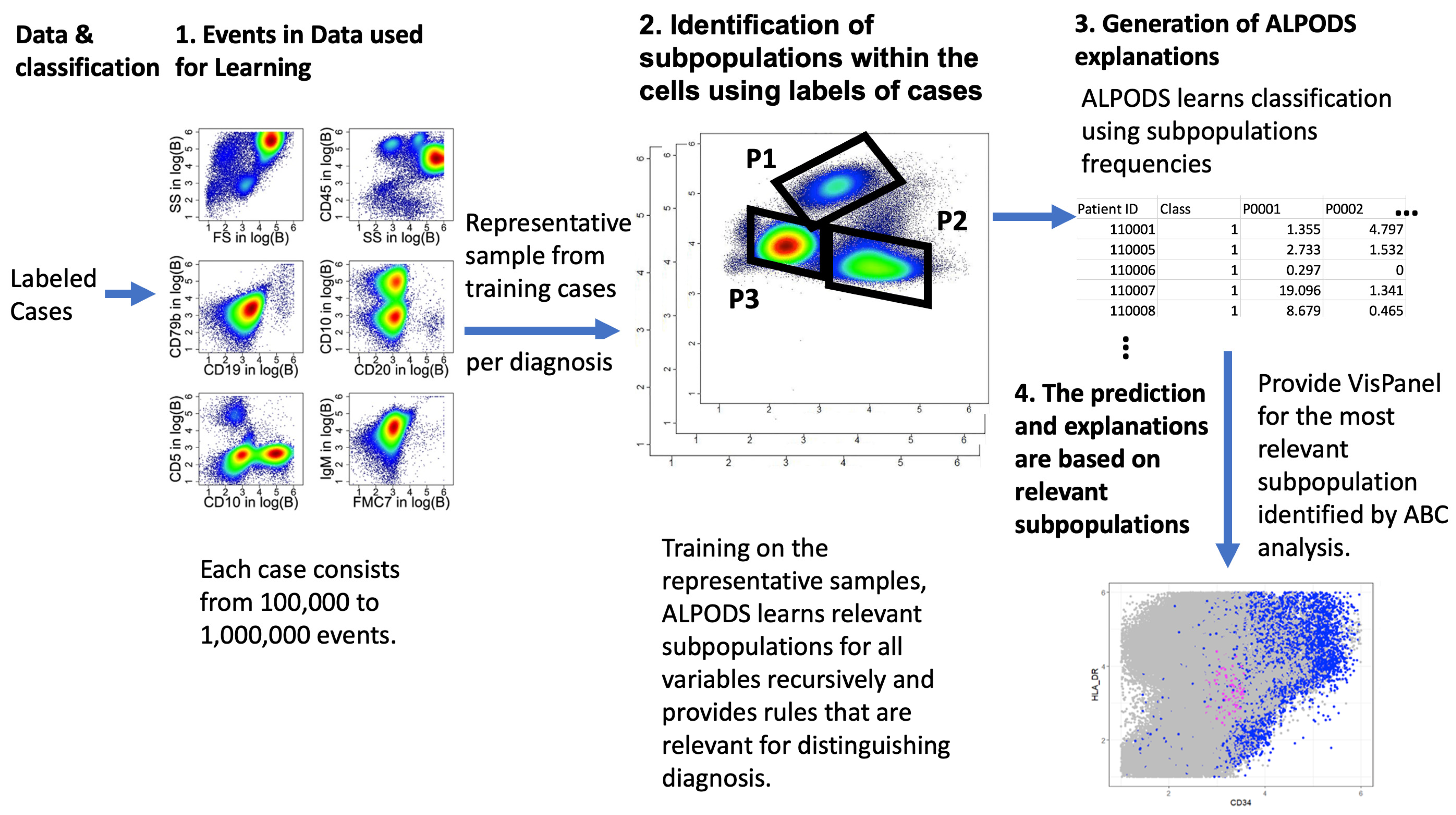
This work proposes a symbolic ML algorithm (algorithmic population descriptions (ALPODS)) that produces and utilizes user-understandable knowledge for its decisions. The algorithm is tested on a typical ML example and two multiparameter flow cytometry datasets from routine clinical practice. The latter datasets are acquired from two clinical centers (Marburg and Dresden). The problem at hand is deciding the primary origin of a probe: mostly bone marrow (BM) or peripheral blood (PB).

Our key contributions are as follows:

• Algorithmic population descriptions (ALPODS) is a novel supervised explainable AI (XAI) that provides physicians with tailored explanations in biological datasets.
• ALPODS is fast-working and requires for learning only a very low number of cases.
• ALPODS distinguishes normal controls from leukemia and bone marrow from peripheral blood samples with high accuracy.
• ALPODS outperforms comparable systems on several datasets in terms of interpretability, performance, and processing time.
• The XAI was already successfully applied for the hemodilution in BM samples to prevent false negative MRD reports and was able to identify to physicians prior unknown and highly predictive cell populations and improved chronic lymphocytic leukemia outcome predictions.

The proposed algorithm is compared to rule-generating AI systems [24] and decision tree rules [25], as well as recently published rule-generating algorithms for flow cytometry [26,27] which are introduced in the Section 2.

2. Methods

An overview of selected AI algorithms is presented below; these methods produce diagnostic decisions for multivariate high-dimensional data such as flow cytometry data. Such data typically comprise several cases (patients). For each case, a fairly large number of events (cells) ($n \ge \mathrm{100,000}$) are measured. In cytometry, for each cell, the expression (presence) of proteins on its surface is measured (variables). The proteins are genetically encoded by cluster of differentiation (CD) genes [28]. For the data, a classification (diagnosis) into one of k classes is given. Each case (patient) is classified, i.e., assigned to a diagnosis class which is typically encoded as a number from $(1,\dots ,k)$. An important issue regarding the analysis of such data is the automated identification of populations (partitions) in high-dimensional (multivariate) data. Such populations may be either relevant for gating the data, i.e., eliminating unwanted cells or debris [29], or, more importantly, the (sub) populations are relevant for a diagnosis.

In summary, in this particular data challenge, each case is described by many events, and each event is described by several features. However, AI algorithms are used to explain a case’s diagnosis, not an event. For such problems, decision trees or ML methods combined with post hoc explainers are typically used. Hence, the Section 2.1 introduces conventional supervised [19] and unsupervised decision trees [25]. The Section 2.2 introduces the more general concept of combining an ML system based on a large number of degenerate decision trees = random forest (RF) with a post hoc explainer, representing an approach for extracting explanations based on a learned model [30]. Finally, a high-performing ML model (RF) with a conventional post hoc explainer based on a linear model with LASSO regularization [24] is presented. For this type of approach, a variety of alternatives are proposed (see [31]).

The Section 2.3 introduces two typical domain-specific algorithms used in flow cytometry. The first one, called SuperFlowType, constructs event hierarchies to provide the best population selection strategies for identifying a target population at the desired level of correlation with a clinical outcome by using the simplest possible marker panels [26]. The second algorithm is called FAUST [32], which delivers descriptions of many populations that are relevant for a particular disease [33].

2.1. Supervised and Unsupervised Decision Trees

XAI algorithms often use either explicit or implicit decision trees. Decision trees are especially popular for medical diagnosis because they are assumed to be easy to comprehend [34]. Decision trees consist of a hierarchy of decisions. At each (decision) node of the tree, a variable ($CDxxx$) and a threshold t are selected. The two possibilities “$CDxxx \le t$” vs. “$CDxxx>t$”, split the considered dataset into two disjunct subsets. For each of these possibilities, descendants are generated in the tree. Different decision tree algorithms use different approaches to select the decision criterion, i.e., the variable $CDxxx$ and the threshold t (selection criterion). The construction process starts with a complete dataset and typically ends if either a descendant node contains cells of only one class (the same diagnosis) or a stopping criterion regarding the size of the remaining subsets is reached. Decision trees are typically supervised algorithms that are trained on a labeled dataset; i.e., for the selection and stopping criteria, predefined classifications (diagnoses) of the labeled cases are needed. A popular decision tree algorithm is CART [19]. CART is used in this work as a performance baseline. We use the CART implementation in the form of the “rpart” R package that is available on the CRAN (https://CRAN.R-project.org/package=rpart) (accessed on 1 January 2020) in this work.

As prime examples in the domain of unsupervised decision trees for which labeled data is not used, the FAUST [32] and eUD3.5 algorithms [25] are selected. FAUST [32] produces a forest of unsupervised decision trees. FAUST is described in detail in Section 2.3. Loyola-González et al. proposed an unsupervised decision tree algorithm called eUD3.5 in 2020 [25]. eUD3.5 uses a splitting criterion based on the silhouette index [25]. The silhouette index compares a cluster’s homogeneity with other clusters’ heterogeneity levels [35]. In eUD3.5, a node is split only if possible descendants have a better splitting criterion than the best criterion found thus far. This leads to a decision tree that is based on cluster structures (homogeneity) and not on the diagnosis. A cluster (subpopulation) is labeled with a particular diagnosis produced by the majority of the members in the subpopulation. In eUD3.5, 100 different trees are generated, their performance is evaluated, and the best-performing tree is kept. The user can specify the number of desired leaf nodes (stopping criterion). If the algorithm produces more leaf nodes than the value specified by the user, the leaf nodes are then combined using k-means. No open-source code was referenced in [25]. A direct request for the source code was unsuccessful. The authors provided no suitable code for Python, MATLAB, or R. Therefore, all eUD3.5 results are taken from [25].

Other alternatives either do not provide their source codes [36] or are unable to process $n>\mathrm{100,000}$ events per case if the run time is limited to 72 h or less [37,38].

2.2. Random Forest and Gradient Boosting with LIME (RF-LIME, Xgboost-LIME)

There is a widespread belief that black-box models perform better than understandable models [9]. Hence, one of the allegedly best-performing ML algorithms, a random forest (RF), was selected [5,6] to investigate this claim. In addition, the chosen Open MP implementation of the RF (see Supplement SI SA for details) used here computes results very efficiently, which is often a requirement in the medical domain. An RF uses many simple decision trees, for which the training data of each tree are randomly subsampled from the full data [39]. A random subset of the variables is evaluated at each decision node. The splitting criterion is usually the same as that in CART [19,40]. Many small trees (typically, $n_{tree}=500$) are considered (forest), and they produce many individual classifications. The forest’s classification is determined by the majority vote of these tree classifications. For explanations, i.e., population rules, the LIME algorithm [24] was used because it is a well-known representative post hoc explainer [41]. In comparison with alternative post hoc explainers [42], LIME produces substantially lower explanation variability from case to case, which is required for understandability. Additionally, our inclination towards LIME over other local post-hoc explainer methods is grounded in the capability of LIME to provide explicit rules. LIME reduces a decision tree to a k-dimensional multivariate regression model. The user must provide the number of variables k used for the regression. From this model, a set of conditions was extracted. The detailed parameter settings and implementation of LIME are described in Supplementary Section SA (SI SA).

As an alternative to RF, Gradient Boosting is a machine learning ensemble technique that builds a predictive model in the form of an ensemble of weak learners, typically decision trees, to sequentially correct errors of the preceding models. The algorithm optimizes by fitting each subsequent model to the residuals of the combined predictions. This iterative process helps create a robust and accurate predictive model [43]. One of the most popular implementations of gradient boosting is the Xgboost algorithm, which has shown outstanding performance in various machine learning tasks [44,45].

2.3. Comparable XAI Methods Used in Flow Cytometry

To conduct a close comparison with our approach, two published methods that operate on flow cytometry data and produce descriptions for subpopulations are described: Supervised FlowType/RchyOptimyx (SuperFlowType) [26,27] and FAUST [32]. Both methods claim to produce XAI systems.

The FlowType [26,27] algorithm consists of a brute force approach that exhaustively enumerates all possible population descriptions defined by all CD variables. For each variable $CDi,$ three different situations are considered: $CDi+, CDi-$, and no $CDi$ condition. The thresholds for the plus ($+$) and minus ($-$) comparisons are calculated by a one-dimensional clustering algorithm using two “subpopulations”: the low range vs. the high range of the variable. Either k-means [46] or flowClust [47] is used as the decision algorithm for the low/high regions. FlowType generates rules for all possible combinations of conditions in all d variables. For d variables and the three possibilities (not used, $+$ and $-$), this results in $p=3d$ populations. For a typical state-of-the-art flow cytometry dataset with $d=10, p=310=59049$ possible cell populations need to be considered. To reduce the number of cell populations, the RchyOptimyx algorithm is applied [26,27]. RchyOptimyx applies graph theory, dynamic programming, and statistical testing to identify the best subpopulations, which are added to a directed acyclic graph (DAG) as representations of hierarchical decisions. SuperFlowType has been used to evaluate standardized immunological panels [48] and to optimize the lymphoma diagnosis process [49]. On the FlowCAP benchmarking data, the application of SuperFlowType resulted in an F measure of 0.95 [50], and the algorithm provided a statistically significant predictive value for the blind test set [51]. O’Neill et al. [27] claimed that SuperFlowType is able, within the memory of a common workstation (12 GB), to analyze 34-marker data. For the datasets used here, the computational load required for the application of SuperFlowType was observed to be extremely high (see Section 5).

The FAUST algorithm consists of two phases [32]. A feature reduction method is applied in the first phase. All possible combinations of three CD markers are considered. A combination is termed “reasonable” if Hartigan’s dip test [52] rejects the unimodality of the distributions. All reasonable combinations are added to a decision tree for a particular case (patient), which was called the “experimental unit” in [32]. The distribution of the depth in which a particular marker combination is observed across all decision trees of all experimental units is recorded. Features with shallow depth values are removed from further consideration (feature selection). During the second phase, the remaining decision trees are pruned by their frequencies of phenotype occurrence across different cases. Each subpopulation in FAUST is described in the form of a set of $CDi+, CDj-$ conditions.

2.4. ALPODS–Algorithmic Population Descriptions

The ALPODS algorithm is constructed as a Bayesian decision network in the form of a directed acyclic graph (DAG). The decision network is recursively built as follows. First, a variable is selected for the current node o of the DAG. The conditional dependencies are evaluated for choosing a variable by using the Simpson index (S). S represents the expected joint probability that two entities taken from the population represent the same type or different types. It is calculated as the conjunction of the probability that an entity belongs to a particular population and the probability that the entity does not belong to the population. This can also be interpreted as the probability that two randomly chosen events do not belong to the same subpopulation. S is biologically inspired by the concept of expected heterozygosity in population genetics and the probability of an interspecific encounter [53]. Conditional dependencies are modeled by using Bayes’ theorem [54] on the probability distribution of the parent node and the probability distribution of the decedent node. The use of Bayesian decisions ensures that the optimal decision is produced in terms of the cost (risk) of a decision [55]. The details of the DAG construction process are described in the pseudocode of Algorithm 1.

Algorithm 1: ALPODS
DAG = GrowDAGforALPODS(DAG,CDi,depth,Population,Classification)
Input:
	DAG
	CDi
	depth
	Population
	Classifcation
1:	if Termination(depth, size(Population), Classification) then
2:		leafLabel = classify(Population, Classification)				▷ Majority vote
3:		DAG = AddLeafToDAG(DAG, leafLabel)				▷ DAG is complete at this leaf
4:	else					▷ Termination not reached
5:		for each variable CDi do
6:			for each plausible condition cond do
7:				Let cond(Population) be the subpopulation resulting from the application of cond.
8:				Use the probability distributions PDF(Population) and PDF(cond(Population))
9:				to calculate a decision on membership using theorem of Bayes
10:				⇒ ClassOfSubpopulation
11:				S(CDi) = SimpsonIndex(Population, cond(Population))
12:				if Significant(S(CDi)) then
13:					AddEdgeToDAG(cond(Population),Label=”cond on CDi”)	▷ Note: edge is only added if it is not already descendent of current DAG
14:					DAG = GrowDAGforALPODS(DAG,CDi,depth+1,Subpopulation,ClassOfSubpopulation)		▷ Expand the DAG recursively
15:				end if		▷ Only for suitable S
16:			end for			▷ For all conditions
17:		end for				▷ For all variables
18:	end if					▷ Expansion of the DAG
Used Procedures:
1:	Termination()                             ▷ Is true if depth size or size exceeds limits or classification contains only one class
2:	AddLeafToDAG()                                            ▷ Adds a leaf node to the DAG
3:	AddEdgeToDAG()                         ▷ Adds edge with label, edge is only added if it is not already descendant of current DAG
4:	Significant()                                                 ▷ Threshold for S
5.	SimpsonIndex()                                           ▷ Computes the Simpson index S

Second, edges are generated and associated with conditional dependencies on descendant nodes. Third, the recursion process stops when a stopping criterion is fulfilled or when DAG construction is recursively applied to all descendant nodes. Recursion starts with the complete dataset as the population. Recursion stops when the class labels are identical for all members of a subpopulation, or the size of a subpopulation is below a predefined fraction of the data, typically 1%. This results in a Bayesian decision network that is able to identify subpopulations within the cells. A comprehensive overview of Bayesian networks in comparison with decision trees can be found in [56]. To explain the subpopulations, the decisions are summarized in explanations. Following the idea of fast and frugal trees [57], the sequence of decisions produced for a population is simplified into an algorithmic population description: all Bayesian decisions, i.e., all conditions that use the same marker, are simplified into a single condition (see below). This describes an interval within the range of this marker. The relevance of the subpopulation for diagnosis purposes is assessed by an effect size measure [58]. By default, the absolute value of Cohen’s d is used [59]. Calculated ABC analysis [60] computed on the effect sizes is recursively applied to select the m most relevant small subpopulations until a preset number of populations is reached, which lies within the miller optimum m of human understanding, i.e., $m=7 \pm 2$ [23]. The simplification step aims to describe a population that is understandable by human experts. The subpopulation descriptions are presented to the domain expert, who is asked to assign a meaningful name for each of the relevant populations.

Explanations of XAI are usually tailored for data scientists as rules and conditions instead of being meaningful to a domain expert [61]. There it is apparent that rules with conditions resulting from an XAI system alone are insufficient to understand the subpopulation selected by the rule. Instead, meaningful explanations should be generated in the “language” of the domain expert [62,63]. Consequently, to address the “meaning” of a certain cell population, a matrix of class-colored scatterplots called visualization panel (VisPanel) was presented to the clinical experts in their typical working environment of Kaluza Analysis Software 2.1 (https://www.beckman.de/en/flow-cytometry/software/kaluza) (accessed on 1 December 2020). As this is propriety software, the population figures in the Section 5 are generated in R. 4.1.1 using the R package “DataVisualizations” available on CRAN [64]. The size and layout of the VisPanel can be determined by the experts in the same way that they normally operate in everyday clinical routines. The complete workflow of ALPODS learning is outlined in Figure 1.

Alternatively, it can be determined by the largest absolute probability differences $(ProbDiffs$). $ProbDiffs$ are calculated for all pairs ($X$,$Y$) of the $d$ variables in the data. For each pair ($X,Y$) of variables, the probability density of a class $c$, called $p(X,Y|c$), is estimated using smoothed data histograms (SDHs) [65]. With this, the absolute probability difference results in $ProbDiff(X,Y,c))=\left|SDH(X,Y|c) – SDH\left(X,Y\left|not\right(c)\right)\right|$.

The computed ABC analysis [60] is applied to the ProbDiffs. The A-set, i.e., the set containing the largest few populations, is selected through the computed ABC analysis, and the ProbDiffs of set A constitute the VisPanel. The class with the highest class probability (for example, BM in Rule 1) is depicted by placing red dots on top of the data outside of the class (PB data in the example). This differential population visualization (DIPOLVIS) method allowed the clinical experts to understand all presented populations and to assign meaningful descriptions to each XAI result. In the above case of Rule 1, population one was identified as “myeloid progenitor cells”.

For example, for the rule “Rule 1”, events relevant to BM are in Population 1 (“SS++ and CD33+ and CD13”); the corresponding VisPanel is shown in Figure 2. The events of “Population 1” are marked in red. Population 1 cells occur in BM probes with an average rate of 43% and in PB with a rate of 5%. The left panel of Figure 2 reveals that the cell population is located in the area of myeloid cells with high side scatter and forward scatter (SS and FS, respectively), apart from lymphocytes and monocytes. The middle panel reveals that the cell population has dim CD45 expression within the myeloid cells. Finally, Population 1 can be identified as myeloid progenitor cells (e.g., myocytes) because of its weak CD13 expression and strong CD33 expression (right panel).

Combining the relevant population with an XAI diagnostic system is based on fuzzy reasoning [66]: the relative membership fractions of the relevant subpopulations are calculated on a selected subset of patient data (extended learning set). Fuzzy membership functions are calculated as the posterior probabilities. Figure 3 shows an example of this approach. On the left panel of Figure 3, the probability distribution functions (PDFs) of the SS variable for a particular subpopulation of the data are shown.

Bayes’ theorem defines the shape of the fuzzy membership function for “SS+ in BM”, with many (“SS”, ”BM”) instances. According to Bayes’ theorem, the decision limit is shown as a black line. This can be used for the calculation of the SI index and for the simplification of the description of a particular population, as stated above. For example, if another condition imposed on SS for BM is less restrictive, that condition can be omitted. Within the SS range of 2.4 to 3.2 in the example of Figure 3, the membership function is indecisive, expanding the diagnostic capabilities of the XAI system. The fuzzy conjunction of all single XAI experts determines the classification (diagnosis). This results in a set of XAI experts for each of the populations.

The key advantage of this approach is that both the pros and cons of a diagnosis can be explained to the domain expert in understandable terms. For example, an explanation of why a probe contains more PB than BM can be seen as “many (thrombocyte aggregates) and few (progenitor B cells)”. The functions many and few are defined as fuzzy set membership functions [66]. The fuzzy rules can be used in a Mamdani-style fuzzy reasoning system [66]. A critical review of these systems states: “Mamdani systems have proven successful for function approximation in many practical applications […] Their success is mainly derived from two characteristics that are very convenient for this objective: Mamdani systems are universal approximators and can include knowledge in the form of linguistic rules that can be used for local fine-tuning.” See also [67].

3. Data Description

All XAI algorithms were tested on a synthetic dataset derived from a well-known ML dataset (Iris) and three different flow cytometry datasets. The first two datasets consisted of samples of either peripheral blood (PB) or bone marrow (BM from patients without any signs of BM disease at two different healthcare centers, University Clinic Dresden and University Clinic Marburg). The manual distinction between such samples poses a challenge for domain experts. The third dataset contained healthy BM samples and leukemia BM samples because the diagnosis of leukemia based on BM samples is a basic task. For details about the measurement process and the structures in the data, we refer to [68].

The synthetic dataset served as a basic test of the performance of the introduced algorithms. As stated in the data description [68], the flow cytometry data were derived from originally obtained diagnostic sample measurements to obtain acute myeloid leukemia (AML) information at the minimal residual disease (MRD) level (cf. [69,70]). For clinicians, whether the BM samples of patients with hematological diseases are diluted with PB is an essential question for correctly assessing MRD statuses. Domain experts (i.e., clinicians) distinguish PB samples from BM samples and leukemia BM samples from nonleukemia BM samples based on biological cell population distributions by looking at two-dimensional scatter plots, i.e., clear, straightforward patterns in data that have biological meanings and are visible to the human eye (cf. [71]). This means that the cases of each sample can be used to benchmark ML methods (cf. [72]). Three types of XAI method assessments were performed using the data: performance, understandability, and processing time assessments.

3.1. Synthetic Data with Gaussian Noise Derived from Iris

The Iris dataset describes three types of Iris flowers (150 samples in total) [73]. The dataset consists of 50 samples from each of three species: Iris setosa, Iris virginica, and Iris versicolor. Four features are given for each sample: the lengths and widths of the sepals and the lengths and widths of the petals. The setosa class is well separated from the other classes, but the other two classes, virginica and versicolor, overlap [74]. This presents “a challenge for any sensitive classifier” [75].

Due to the challenge of clinical datasets being expensive and many XAI algorithms starting with a simplified validation case, we derived a synthetic dataset from Iris to adapt to the given data challenge. To obtain sufficiently large training and testing datasets, Gaussian noise with zero means and small variances N(0,s) was added to the data values. Ten percent of the variance (s²) in each of the four variables was used. This procedure (jittering) was applied ten times, resulting in 1500 cases divided into equal-sized training and test sets with n = 750 cases each. To ensure that the jittered data were structurally equivalent to the original Iris dataset, a random forest (RF) classifier was trained with the jittered data. This (RF) classifier was able to classify the jittered data with an accuracy of 99%. i.e., the jittered data could be used for training and testing XAI algorithms along with the original Iris data.

3.2. Marburg and Dresden Data

A retrospective reanalysis of flow cytometry data from blood and BM samples was performed according to the guidelines of the local ethics committee. Detailed descriptions of the flow cytometry datasets and their availability are described in [70].

The Marburg dataset consisted of N = 7 data files (samples) containing event measures from PB and N = 7 data files for BM. The Dresden dataset comprised N = 22 sample files for PB and N = 22 samples for BM. Each sample file contained more than 100,000 events for a set of features extensively described in [68]. It should be noted that the goal of the investigated XAI algorithms is not to predict single events within each data file but to predict the class of the data file itself. The classifications for the events were derived from the classes of the data files (BM or PB).

The files were randomly subsampled to obtain the training data as follows. We took from each file the same number of events and joined them into a single training dataset. The Marburg training set contained n = 700,000 events, i.e., <30% per data file was taken. The Dresden dataset contained n = 440,000 events, i.e., a 10% sample per data file was taken.

The XAI algorithms used the training data to generate populations and corresponding decision rules. XAI system training was performed in an event-based manner on the balanced sample described above. Testing was performed on the sample data files for which a decision (BM or PB) was calculated as a majority vote of the population classifiers.

The exception was “full annotation using shaped-constrained trees” (FAUST), which served as a feature extraction method. The rule-based explanations generated for the training files were applied to the sample files, resulting in cases (sample files) of extracted cell count features (rules). These cell counts were used as the inputs of RFs (SI A for the specific algorithm), for which the target was the class of the sample file. For the N = 14 sample files of Marburg, leave-one-out cross-validation was performed, and for the other datasets, n-fold cross-validation was performed on 50% of the test data after learning the RF classifier on 50% of the training files. To provide an easy example of providing explanations with ALPODS, another dataset with N = 25 healthy BM samples and N = 25 leukemia BM samples was used.

4. Quality Assessment

XAI systems deliver a set of $\mathrm{S}\mathrm{P}=\#p$ subpopulations (partitions) of a dataset that are presumably relevant for distinguishing a particular diagnosis c from all data that do not fit into the diagnosis class (not $c$). Therefore, the first criterion to be applied to an XAI system is to measure how each subpopulation matches the classification results. This is usually measured using accuracy, which is the percentage of subpopulation elements that are consistent with the diagnosis class [76].

The second aspect of XAI systems is the question of understandability. Understandability by itself is a multifactor issue (see [77] for a discussion). However, one of the basic requirements for understandability is the simplicity of an explanation [22]. This can be measured as follows. XAI systems deliver not only a number of subpopulations $\#p$ but also rules that describe the content using a number of conditions ($\#cond$). To understand the results of an XAI system, both #p and #cond must be in human-understandable ranges. According to one of psychology’s most often cited papers, optimal memorization and understanding in humans is possible if the number of items presented is approximately $n_{item}=7$ (the Miller number) [23]. Consequently, the sizes of the results, $\#p$ and $\#cond$, of an XAI system are considered to not be understandable if they are either trivial with $n_{item}<2$ or too complex with $n_{item}>14$ [22].

The third aspect of quality assessment considers computation time which was limited to 72 h. Finally, the performance evaluation was performed for each patient sample with the accuracy measure because the numbers of blood samples and BM samples were balanced.

4.1. Evaluation of Randomized Synthetic Data

An RF was constructed using the training dataset ($n=750$). This RF was applied to classify the $n=750$ test data. The accuracy of the RF classifier was evaluated on the test data for 50 rounds of cross-validation. For each case, LIME provided a local explanation through a rule. The casewise rules were aggregated using an algorithm that generates a faceted LIME heatmap. Then, the rules could be extracted from the x-axis of this heatmap (see Supplementary Figure S1, SI SA). For SuperFlowType, three binary classifications, one iris flower type vs. all others, were constructed ($n=250$ cases). Rules were generated by comparing class 1 with the combination of classes 2 and 3, class 2 with classes 1 and 3, and class 3 with classes 1 and 2 and applied to the test dataset (n = 750).

4.2. Evaluation of Flow Cytometry Data

For each method with usable code, the rules for the subpopulations were constructed on the Marburg and Dresden training datasets. Good clinical practice states that the duration of the experiment should be appropriate to achieve its objectives; here, the physicians typically diagnose patients within 24–48 h with conventional personal computers (oral communication with collaborating physicians, see also [78]). Therefore, we limited the computation time for all practical purposes to a maximum of 72 h of high-end parallel computing. The accuracies of the classifiers were calculated on the sample data files using up to 50 rounds of cross-validation within the time limit.

Neither RF_LIME nor SuperFlowType was able to compute results on a personal computer (iMac PRO Apple Inc. 1 Apple Park Way Cupertino, CA 95014 USA, 32 cores, 256 GB of RAM) in 72 h of computing time. Therefore, to be able to compute results, the M32ms Microsoft Azure Cloud Computing system consisting of 32 cores and 875 GB of RAM (9.180163 EUR/h) was used. Nevertheless, neither the RF nor the FlowType methods (RF_LIME and SuperFlowType) were able to provide results for the full training set of the data. Thus, a $20\%$ sample was used, which resulted in a 40 h computational time for RF_LIME and a 24 h computational time for SuperFlowType per trial in the case of the Marburg dataset. For the Dresden dataset, RF_LIME did not yield results in the required time frame. Computing results for SuperFlowType took 24 h with the procedure defined above.

5. Results

The algorithms introduced in the prior sections were applied to the synthetic data with Gaussian noise derived from Iris. This serves as a basic test of their performance because the datasets for human medical research are limited and not available in large quantities. In contrast, Iris is a well-known biological dataset for which the performance of algorithms is expected to be high. The data comprised three distinct classes ($k=3$), which needed to be diagnosed using the $d=4$ variables.

Table 1. The average running time, the number of subpopulations SP, and the number of explanation rule conditions required by each of the XAI algorithms on the synthetic data with Gaussian noise derived from Iris. The CART baseline [19] had an accuracy of $98\%$ and required four rules. CART was computed with the “rpart” R package available on the CRAN “https://CRAN.R-project.org/package=rpart”, accessed on 1 January 2020). The results of eUD3.5 are cited from [25].

Synthetic Data with Gaussian Noise	eUD3.5	FAUST *	RF-LIME	Xgboost-LIME	Super FlowType	ALPODS
Processing Time	<1 min	<1 min	<1 min	<1 min	<1 min	<1 min
No. Cross-Validation Steps	50	*	50	50	50	50
Max no. of SP	15	4	14	3	30	5
Mean no. of SP	8 ± 3.4	4	6 ± 3.2	3	7 ± 3	2 ± 1
Max no. of Conditions for a SP	4	4	2	2	4	4
Mean no. of Conditions for a SP	2 ± 1.1	4	2 ± 0.5	1.5	3 ± 0.8	2 ± 0.7
Accuracy Performance	98 ± 0.5	64 *	96.3 ± 1.4	99 ± 0.7	80 ± 10	96 ± 0

* For FAUST, a classifier could not be learned. Hence, the accuracy between the given partitions and the FAUST-generated subpopulations was measured by the procedure described in the “FCPS” R package on the CRAN [79].

shows that the accuracies of all algorithms except SuperFlowType exceeded $90\%$. The largest differences were observed in the number of identified partitions and the number of conditions required for the description of a partition. However, all algorithms delivered sufficiently simple descriptions with typically fewer than nine partitions. Surprisingly, the partitions delivered by FAUST did not match the partitions of the synthetic data, meaning that the descriptions were not useful.

The eUD3.5 algorithm could not be transferred to the Marburg and Dresden datasets because no source code was accessible. For each method with usable open-source code, subpopulation rules were constructed on the two training datasets (for details, see Section 3). The physicians required that computational time per method and experiment should be limited to 72 h. The accuracies achieved by the resulting classifiers on the test data were calculated on the respective sets of patient data files using up to 50 rounds of cross-validation within the time limit. Neither RF_LIME nor SuperFlowType were able to compute results on a personal computer. Nevertheless, neither the RF nor FlowType submethod (of RF_LIME and SuperFlowType, respectively) provided full results on the training set. Thus, a $20\%$ sample was used, which resulted in a 40 h computation time for RF_LIME and a $24$ h computation time for SuperFlowType in the case of the Marburg dataset.

Table 2. The average running time, the number of subpopulations (SP), and the number of explanation rule conditions required by each of the XAI algorithms on the Marburg dataset. The CART baseline [19] had an accuracy of 50% and required six rules. CART was computed with the “rpart” R package available on the CRAN “https://CRAN.R-project.org/package=rpart”, accessed on 1 January 2020).

Marburg Dataset	RF-FAUST	RF-LIME	Xgboost-LIME	SuperFlowType	ALPODS
Processing Time	<1 min	72 h	15 min	24 h	1 min
No. Cross-Validation Steps	*	2	50	3	50
Max no. of SP	79	40	2	5486	5
Mean no. of SP	79	21 ± 11.6	2	2744 ± 1583	3 ± 1
Max no. of Conditions for a SP	8	2	80	10	6
Mean no. of Conditions for a SP	8	2 ± 0.5	80	10	5 ± 0.8
Accuracy Performance	92	80.0 ± 0.0	80.8 ± 13.7	71.6 ± 15.9	96.9 ± 0.9

* Leave-one-out cross-validation was employed.

shows these results.

For the Dresden dataset, RF_LIME did not obtain a result in the required maximum duration of the experiment. Computing the results for SuperFlowType took 24 h, again with the procedure defined above.

Table 3. The average running time, the number of subpopulations (SP), and the number of explanation rule conditions required by each of the XAI algorithms on the Dresden dataset. The CART baseline [19] had an accuracy of 46% and required nine rules. CART was computed with the “rpart” R package available on the CRAN “https://CRAN.R-project.org/package=rpart”, accessed on 1 January 2020).

Dresden Dataset	RF-FAUST	RF-LIME	Xgboost-LIIME	SuperFlowType	ALPODS
Processing Time	17 min	>72 h	36 h	24 h	1 min
No. Cross-Validation Steps	50	-	1	1	50
Max no. of SP	43	-	2	1456	5
Mean no. of SP	43	-	2	729 ± 420.5	3 ± 1.4
Max no. of Conditions for a SP	8	-	80	10	6
Mean no. of Conditions for a SP	8	-	80	10	4 ± 1.1
Accuracy Performance	96 ± 0.06	-	80.8 ± 8.3	70	96.8 ± 0.9

presents these results. Contrary to the compared algorithms, ALPODS finished after 1 min of CPU time on the iMac PRO.Therefore, only ALPODS was able to perform the desired 50 cross-validations. For the Marburg dataset, ALPODS identified five relevant populations for distinguishing between BM and PB. Utilizing visualization techniques, clinical experts could understand the population and identify the following cell types in the population.

FlowType started with all $3d$ possible conditions for all d variables. For the flow cytometric data, this meant more than $\mathrm{50,000}$ populations. Optimix reduced this to approximately $8000$ populations, and the subsequent ABC analysis, which took the significance of the subpopulations into account for diagnosis purposes, reduced this to an average of $2744$ populations. However, this number of subpopulations was too large to even look for further explanations. Only a fraction of the results had acceptable accuracies exceeding $80\%.$ The number of subpopulations identified by RF_LIME typically ranged from $20$ to $40$.

Contrary to the claim of the authors of FAUST that “it has a general purpose and can be applied to any collection of related real-valued matrices one wishes to partition” [32], FAUST failed to reproduce the cluster structures of the synthetic dataset derived from iris (0.64 accuracy). As their initial benchmark was neither unbiased nor compared with state-of-the-art clustering algorithms (cf. the discussion in [72]), further studies would be required to investigate whether FAUST is able to explain the given structures in data. Although the RF classifier yielded a performance nearly equal to that of ALPODS for the flow cytometry datasets, a large number of populations with eight conditions for each population were too complex to be understandable by domain experts without additional algorithms for selecting appropriate populations. Even then, describing each population by eight conditions for each condition containing up to three thresholds seems unfeasible. The results indicate that FAUST is probably not very useful for discovering knowledge in flow cytometric datasets. Moreover, its computational time increased on larger training datasets in comparison with ALPODS.

The results obtained on the Dresden dataset were similar. For the five populations identified by ALPODS (see

Table 4. Description rules generated by ALPODS for the Marburg dataset, which could be described by human experts, and their PB and BM occurrence frequencies. Abbreviations: not(-) means weak staining, considered unspecific, 0 means centered around zero.

Pop No.	Cell Types	Description Rule	Frequencies in [%]
			PB	BM
1	Myeloid progenitor cells	SS+, CD33+, CD13-	5.0	43.0
2	Subcellular events and aggregates	SS-, HLA_DR-, CD45-, CD117not(+), CD33-	19.0	1.0
3	Progenitor B cells	SS-, HLA_DR+, CD4not(+)	0.3	2.0
4	Thrombocyte aggregations	SS-, HLA_DR-, CD13-, CD117not(−), CD34not(−), CD117not(+)	4.2	0.5
5	CD34+ early progenitor cells	SS (0), CD45-, CD34+	1.0	8.0

), the main cell types could be identified (see

Table 5. Description rules generated by ALPODS for the Dresden dataset, which could be described by human experts, and their PB and BM occurrence frequencies. Abbreviation: not(-) means weak staining, considered unspecific.

Pop No.	Cell Types	Description Rule	Frequencies in [%]
			PB	BM
1	Myeloid progenitor cells	FS+, CD45-, CD13-	2.0	26.9
2	Mature granulocyte subset	SS+, CD7not(−), CD117+, CD13+	13.0	2.9
3	T cells	SSnot(−), below average CD33, CD45+, CD13-	12.2	2.1
4	Granulocytes subset	Below average HLA_DR, below average CD33, above average CD7, CD117-, SS+, above average CD13	9.1	1.9
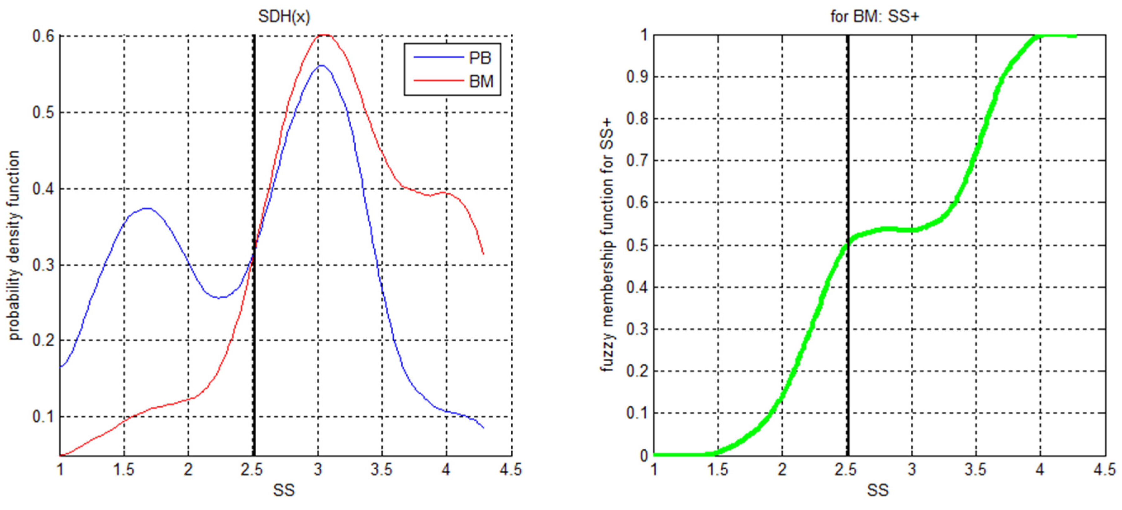
5	Hematogones with lymphocyte subset	CD33-, FS-, CD45not(+), CD13-	2.6	8.6

). For example, in ALPOD’s descriptions for the identified subpopulations “Progenitor B cells” and “Thrombocyte aggregations”, one of the terms in the description is “$SS-$“ (see Table 4). The calculatable form of this expression is derived from the distribution as depicted in Figure 3. The lower part of the distribution is the negation of Figure 3 right panel, i.e., the smaller the SS value is compared to the Bayes decision limit of $2.5,$ the more the condition $SS-$ is fulfilled.

In sum, blood stem cells were located in the BM niche and gave rise to myeloid progenitor cells (population 1). At the developmental maturation stage of granulocytes, these cells were released into the PB (populations 2 and 4). T cells were derived from the thymus and proliferated in the PB upon stimulation following infection (population 3). Therefore, these cell types predominantly occurred in the PB. Hematogenous cells are B-cell precursor cells that were found almost exclusively in the BM (population 5). However, due to active cell trafficking, there was no strict border between the two organic distributional spaces.

We further sought to verify the principle of the algorithm with another dataset and compared BM samples diagnosed as normal (healthy) BM (N = 25) and samples with leukemia cell infiltration (N = 25); see [68] for a detailed description. The results are summarized in

Table 6. Overview of datasets and accuracy results. CART was used as a baseline. The physicians require that the duration of the usage of a method should not take longer than 72 h. Otherwise we note that it is not computable. The number of explanations is defined as the average number of subpopulations multiplied by the average number of conditions.

Method/Description	Synthetic Data	Marburg	Dresden	Leukemia
Number of Cases per class	(50, 50, 50)	(7, 7)	(22, 22)	(25, 25)
Average number of events per case	1500	330,000	579,000	406,000
Accuracy of Baseline (CART)	98	50	46	90
Accuracy of RF-FAUST	64 *	92	96 ± 0.06	98 ± 0.5
No. Explanations of RF-Faust	4 × 4	8 × 79	8 × 43	8 × 212
Accuracy of RF-LIME	96.3 ± 1.4	80.0 ± 0.0	Not computable	Not computable
No. Explanations of RF-LIME	6 × 2	21 × 2	Not computable	Not computable
Accuracy of SuperFlowType	80 ± 10	71.6 ± 15.9	70	Not computable
No. Explanations of SuperFlowType	7 × 3	2744 × 10	729 × 10	Not computable
Accuracy of ALPODS	96	96.9 ± 0.9	96.8 ± 0.9	98 ± 2
No. Explanations of ALPODS	2 × 2	3 × 5	3 × 4	2 × 7
Accuracy of Xgboost-LIME	99 ± 0.7	80.8 ± 13.7	80.8 ± 8.3	Not computable
No. Explanations of Xgboost-LIME	1.5 × 3	80 × 2	80 × 2	Not computable

* For FAUST, a classifier could not be learned. Hence, the accuracy between the given partitions and the FAUST-generated subpopulations was measured by the procedure described in the “FCPS” R package on the CRAN [79].

and visualized in Figure 4.

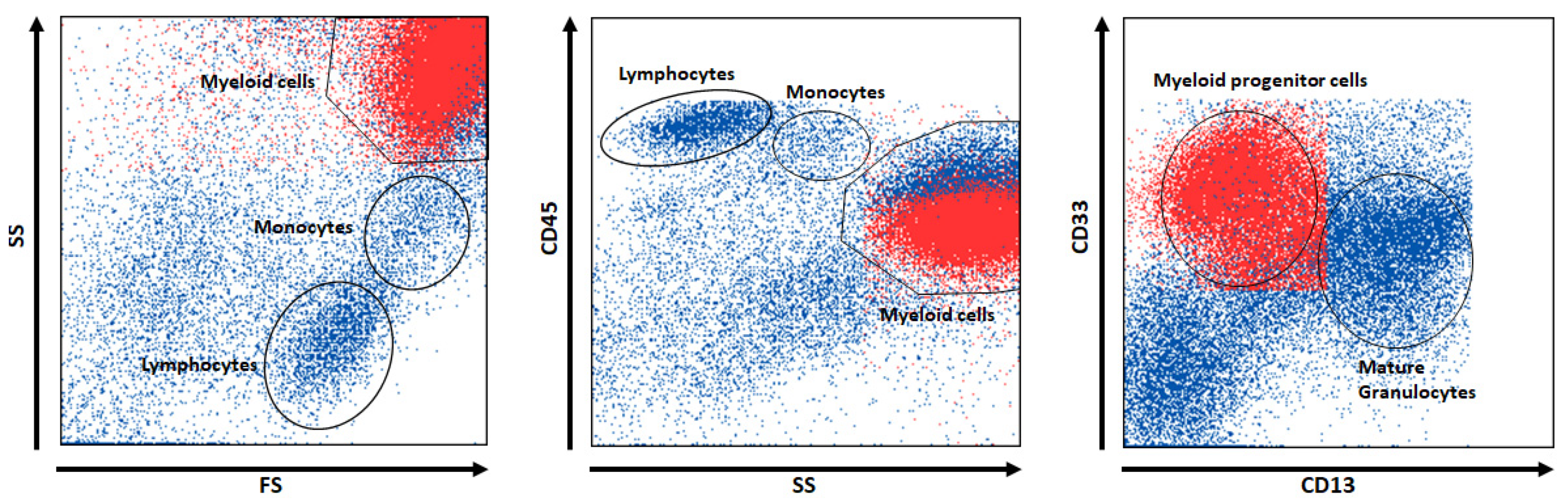
Domain experts assess flow cytometric samples based on biological cell populations with characteristic fluorescence expressions in two-dimensional dot plots, as demonstrated for distinguishing leukemias from normal controls in Figure 5. The results from data scientists can be presented in these two-dimensional dot plots, enabling their plausibility to be verified by domain experts. This approach integrates domain-specific knowledge into the analysis, ensuring that the interpretations are not only statistically valid but also biologically relevant and meaningful.

Within a computation time of several minutes, ALPODS identified a major dominant population labeled “blast cells” by the flow cytometry experts in the VisPanels of Figure 6a,b. The population was described by one explanation, resulting in a $98\%$ classification accuracy. The blast cell population was characterized by a high expression of the antigens CD34 and CD117, while CD45 was only moderately expressed, as depicted in a conventional scatter plot (Figure 6b). “Blast cell” is another term for “leukemia cell”. A blast cell infiltration level $>20\%$ defines the disease “leukemia” as diagnosed out of a BM specimen by physicians. If a second population (magenta in the VisPanels in Figure 6a,b) defined by an additional explanation is considered, the accuracy of the test data is $100\%$. The comparative approach FAUST [32] identified 212 relevant populations after a computation time of 3 h. The application of RFs to these populations resulted in an accuracy of $92\%$ on the test data. The results are summarized in Table 6.

The Applications of ALPODS

The International Prognostic Index (IPI) is used to predict outcomes in chronic lymphocytic leukemia (CLL) based on five factors, including genetic analysis [80]. We aimed to determine if multiparameter flow cytometry data could predict CLL outcomes using ALPODS and explain the results through distinctive cell populations. A total of 157 CLL cases were analyzed, and the ALPODS XAI algorithm was used to identify cell populations linked to poor outcomes (death or first-line treatment failure). ALPODS identified highly predictive cell populations using MPFC data, improving CLL outcome predictions [81].

Minimal residual disease (MRD) detection is crucial for predicting survival and relapse in acute myeloid leukemia (AML) [82]. However, the bone marrow (BM) dilution with peripheral blood (PB) increases with aspiration volume, causing underestimation of residual AML blast amount and potentially leading to false-negative MRD results [83,84]. To address this issue, we developed an automated method for the simultaneous measurement of hemodilution in BM samples and MRD levels [85]. First, ALPODS was trained and validated using flow cytometric data from 126 BM and 23 PB samples from 35 patients. ALPODS identified discriminating populations, both specific and non-specific for BM or PB, and considered their frequency differences. Based on the identified populations, the subsequent Cinderella method accurately predicted PB dilution, showing a strong correlation with the Holdrinet formula [86], and, hence, the methodology can help to prevent false-negative MRD reports.

6. Discussion

AI systems constructed by ML have shown in recent years that these algorithms are able to perform classification tasks with precision similar to that of experts in a domain. Subsymbolic systems, for example, ANNs, are usually the best-performing systems. However, the subsymbolic approach deliberately sacrifices explainability, i.e., human understanding, in a tradeoff with performance. For life-critical applications, such as medical diagnosis, AI systems that are able to explain their decisions (XAI systems) are needed. Here, XAI systems, which identify subpopulations within a dataset that are (first) relevant for the diagnosis process and (second) describable in the form of a set of conditions (rule) that are in principle human-understandable and genuinely reflect the clinical condition, are considered. For such systems, several criteria are relevant. First, from a practical standpoint, the algorithm should be able to finish its task in a reasonable amount of time on typical hardware. Second, the performance achieved in terms of decision accuracy should exceed 80–90%, and third and most importantly, the results must be understandable in the sense that they are interpretable by and explainable to human domain experts.

In this work, we introduced an XAI algorithm (ALPODS) designed for large ($n \ge \mathrm{100,000}$) and multivariate data (d ≥ 10), such as typical flow cytometry data. The distinction between BM and PB served as an example because many approaches have been proposed to solve the problem of BM dilution with PB [86,87]. Holdrinet et al. [86] suggested counting nucleated cells with an external hemacytometer device, while others have suggested running a separate flow cytometric panel to quantify the populations that predominantly occur in the BM or PB areas [87,88]. Of note, the ALPODS algorithm is capable of extracting information about population differences from both datasets, thus making additional external or additional measurements dispensable. In comparison with other state-of-the-art XAI algorithms developed for the same task, ALPODS delivered human-understandable results. Experts in flow cytometry identified the cell populations as “true” progenitor cells, T cells, or granulocytes. Moreover, experts verified that the distribution patterns of these populations in PB and BM were plausible according to the knowledge of hematologists. To achieve enhanced understandability, a visualization tool relying on differential density estimation between the cases in a subpopulation (partition) vs. the rest of the data was essential because it seems that in several domains, visualizations significantly improve the understandability of explanations. For example, in xDNN, appropriate training images are algorithmically selected as prototypes and combined into logical rules (called mega clouds) in the last layer to explain the CNN’s decision [15]. Similar to the VisPanel of the ALPODS method introduced here, the presented rules are human-understandable because they are presented as images. However, the generalization of the explanation process is performed by neural networks’ well-known application of a Voronoi tessellation [89,90] of the projection produced by principal component analysis (PCA) [91]. If a high-dimensional dataset, for example, N > 18,000 gene expressions of patients diagnosed with a variety of cancer illnesses, is considered [72], neither the logical rules consisting of prototypes nor the Voronoi tessellation of PCA would be understandable to a domain expert. Moreover, it is well known that PCA does not reproduce high-dimensional structures appropriately [89], which could lead to untrustworthy explanations.

The XAI expert system constructed using the results of ALPODS was able to correctly distinguish between two material sources by identifying cellular and subcellular events, i.e., BM and PB. In particular, every diagnosis provided by this XAI system could be understood and validated by human experts. Moreover, in line with the argument presented by Rudin [9], the results indicated that a trade-off between understandability and accuracy is not necessary for XAI systems that use biomedical data.

Differentiating between PB and BM is manageable for human experts in the flow cytometry field without AI. Therefore, this problem is perfectly suited as a proof of concept for XAI because it is comprehensible and verifiable to human experts, as we showed here. However, the degree of BM dilution with PB increases with the aspiration volume, causing the residual AML blast amount to be consecutively underestimated. To prevent false-negative MRD results, ALPODS was already applied using a simple automated method for the one-tube simultaneous measurement of hemodilution in BM samples and MRD levels [85].

7. Conclusions

The cell population-based approach of ALPODS is universally applicable for high-dimensional biomedical data and other data and may help answer meaningful questions regarding diagnostics and therapy for cancer and hematological blood and BM diseases. In practice, ALPODS may facilitate the sophisticated differential diagnosis of lymphomas and may help to identify prognostic subgroups. Most importantly, ALPODS reduces the inputted complex high-dimensional flow cytometry data to essential disjoint cell populations. Only this essential information is usable for humans and could assist clinical decisions in the future. ALPODS delivered human-understandable results. One additional advantage of the proposed algorithm is that its computational time is significantly less than that of comparable algorithms. It should be noted that the intended usage of ALPODS will involve datasets in which each case itself comprises many events. In contrast, many typical XAI methods focus on data for which a case is stored within one event described by a set of features. The future scope is to evaluate the diagnostic capabilities of ALPODS for a high number of N > 1000 patients in specific clinical settings and to compare the VisPanel with feature importance methods.

References

1. Keyes, T.J.; Domizi, P.; Lo, Y.C.; Nolan, G.P.; Davis, K.L. A cancer biologist’s primer on machine learning applications in high-dimensional cytometry. Cytom. A 2020, 97, 782–799. [Google Scholar] [CrossRef] [PubMed]
2. Hu, Z.; Glicksberg, B.S.; Butte, A.J. Robust prediction of clinical outcomes using cytometry data. Bioinformatics 2019, 35, 1197–1203. [Google Scholar] [CrossRef] [PubMed]
3. Zhao, M.; Mallesh, N.; Höllein, A.; Schabath, R.; Haferlach, C.; Haferlach, T.; Elsner, F.; Lüling, H.; Krawitz, P.; Kern, W. Hematologist-level classification of mature B-cell neoplasm using deep learning on multiparameter flow cytometry data. Cytom. A 2020, 97, 1073–1080. [Google Scholar] [CrossRef] [PubMed]
4. Murphy, K.P. Machine Learning: A Probabilistic Perspective; MIT Press: Cambridge, MA, USA, 2012. [Google Scholar]
5. Wainberg, M.; Alipanahi, B.; Frey, B.J. Are random forests truly the best classifiers? J. Mach. Learn. Res. 2016, 17, 3837–3841. [Google Scholar]
6. Delgado, M.F.; García, E.C.; Ameneiro, S.B.; Amorim, D.G. Do we need hundreds of classifiers to solve real world classification problems? J. Mach. Learn. Res. 2014, 15, 3133–3181. [Google Scholar]
7. Ultsch, A. The integration of connectionist models with knowledge-based systems: Hybrid systems. In Proceedings of the SMC’98 Conference Proceedings—1998 IEEE International Conference on Systems, Man, and Cybernetics (Cat. No.98CH36218), San Diego, CA, USA, 14 October 1998; pp. 1530–1535. [Google Scholar]
8. Tjoa, E.; Guan, C. A survey on explainable artificial intelligence (XAI): Toward medical XAI. IEEE Trans. Neural Netw. Learn. Syst. 2020, 32, 4793–4813. [Google Scholar] [CrossRef] [PubMed]
9. Rudin, C. Stop explaining black box machine learning models for high stakes decisions and use interpretable models instead. Nat. Mach. Intell. 2019, 1, 206–215. [Google Scholar] [CrossRef] [PubMed]
10. Kahneman, D.; Miller, D.T. Norm theory: Comparing reality to its alternatives. Psychol. Rev. 1986, 93, 136. [Google Scholar] [CrossRef]
11. Sen, S.; Knight, L. A genetic prototype learner. IJCAI 1995, 1, 725–733. [Google Scholar]
12. Nakamura, E.; Kehtarnavaz, N. Determining number of clusters and prototype locations via multi-scale clustering. Pattern Recognit. Lett. 1998, 19, 1265–1283. [Google Scholar] [CrossRef]
13. Vesanto, J. SOM-based data visualization methods. Intell. Data Anal. 1999, 3, 111–126. [Google Scholar] [CrossRef]
14. Thrun, M.C.; Ultsch, A. Uncovering High-Dimensional Structures of Projections from Dimensionality Reduction Methods. MethodsX 2020, 7, 101093. [Google Scholar] [CrossRef]
15. Angelov, P.; Soares, E. Towards explainable deep neural networks (xDNN). Neural Netw. 2020, 130, 185–194. [Google Scholar] [CrossRef]
16. Stöger, K.; Schneeberger, D.; Holzinger, A. Medical artificial intelligence: The European legal perspective. Commun. ACM 2021, 64, 34–36. [Google Scholar] [CrossRef]
17. Adadi, A.; Berrada, M. Peeking inside the black-box: A survey on Explainable Artificial Intelligence (XAI). IEEE Access 2018, 6, 52138–52160. [Google Scholar] [CrossRef]
18. Hayes-Roth, F.; Waterman, D.A.; Lenat, D.B. Building Expert System; Addison-Wesley Publishing Co.: Reading, MA, USA, 1983. [Google Scholar]
19. Breiman, L.; Friedman, J.; Stone, C.J.; Olshen, R.A. Classification and Regression Trees; CRC Press: Boca Raton, FL, USA, 1984. [Google Scholar]
20. Salzberg, S.L. C4.5: Programs for machine learning by J. Ross Quinlan. Morgan Kaufmann Publishers, Inc., 1993. Mach. Learn. 1994, 16, 235–240. [Google Scholar] [CrossRef]
21. Cohen, W.W. Fast effective rule induction. In Proceedings of the Twelfth International Conference on Machine Learning, Tahoe City, CA, USA, 9–12 July 1995; Prieditis, A., Russell, S., Eds.; Morgan Kaufmann: Tahoe City, CA, USA, 1995; pp. 115–123. [Google Scholar] [CrossRef]
22. Dehuri, S.; Mall, R. Predictive and comprehensible rule discovery using a multi-objective genetic algorithm. Knowl.-Based Syst. 2006, 19, 413–421. [Google Scholar] [CrossRef]
23. Miller, G.A. The magical number seven, plus or minus two: Some limits on our capacity for processing information. Psychol. Rev. 1956, 63, 81–97. [Google Scholar] [CrossRef]
24. Ribeiro, M.T.; Singh, S.; Guestrin, C. “Why should I trust you?” Explaining the predictions of any classifier. In Proceedings of the 22nd ACM SIGKDD International Conference on Knowledge Discovery and Data Mining, San Francisco, CA, USA, 13–17 August 2016; pp. 1135–1144. [Google Scholar]
25. Loyola-González, O.; Gutierrez-Rodríguez, A.E.; Medina-Pérez, M.A.; Monroy, R.; Martínez-Trinidad, J.F.; Carrasco-Ochoa, J.A.; García-Borroto, M. An explainable artificial intelligence model for clustering numerical databases. IEEE Access 2020, 8, 52370–52384. [Google Scholar] [CrossRef]
26. Aghaeepour, N.; Jalali, A.; O’Neill, K.; Chattopadhyay, P.K.; Roederer, M.; Hoos, H.H.; Brinkman, R.R. RchyOptimyx: Cellular hierarchy optimization for flow cytometry. Cytom. A 2012, 81, 1022–1030. [Google Scholar] [CrossRef]
27. O’Neill, K.; Jalali, A.; Aghaeepour, N.; Hoos, H.; Brinkman, R.R. Enhanced flowType/RchyOptimyx: A bioconductor pipeline for discovery in high-dimensional cytometry data. Bioinformatics 2014, 30, 1329–1330. [Google Scholar] [CrossRef]
28. Mason, D. Leucocyte Typing VII: White Cell Differentiation Antigens: Proceedings of the Seventh International Workshop and Conference Held in Harrogate, United Kindom; Oxford University Press: Oxford, UK, 2002. [Google Scholar]
29. Shapiro, H.M. Practical Flow Cytometry; John Wiley & Sons: Hoboken, NJ, USA, 2005. [Google Scholar]
30. Lipton, Z.C. The mythos of model interpretability. Queue 2018, 16, 31–57. [Google Scholar] [CrossRef]
31. Lundberg, S.M.; Lee, S.I. A unified approach to interpreting model predictions. In Advances in Neural Information Processing System; Guyon, I., Luxburg, U., Bengio, S., Wallach, H., Fergus, R., Vishwanathan, S., Garnett, R., Eds.; Curran Associates Inc.: Long Beach, CA, USA, 2017; pp. 4765–4774. [Google Scholar]
32. Greene, E.; Finak, G.; D’Amico, L.A.; Bhardwaj, N.; Church, C.D.; Morishima, C.; Ramchurren, N.; Taube, J.M.; Nghiem, P.T.; Cheever, M.A. New interpretable machine-learning method for single-cell data reveals correlates of clinical response to cancer immunotherapy. Patterns 2021, 2, 100372. [Google Scholar] [CrossRef]
33. Vick, S.C.; Frutoso, M.; Mair, F.; Konecny, A.J.; Greene, E.; Wolf, C.R.; Logue, J.K.; Franko, N.M.; Boonyaratanakornkit, J.; Gottardo, R. A regulatory T cell signature distinguishes the immune landscape of COVID-19 patients from those with other respiratory infections. Sci. Adv. 2021, 7, eabj0274. [Google Scholar] [CrossRef] [PubMed]
34. Ripley, B.D. Pattern Recognition and Neural Networks; Cambridge University Press: Cambridge, UK, 2007. [Google Scholar]
35. Rousseeuw, P.J. Silhouettes: A graphical aid to the interpretation and validation of cluster analysis. J. Comput. Appl. Math. 1987, 20, 53–65. [Google Scholar] [CrossRef]
36. Dasgupta, S.; Frost, N.; Moshkovitz, M.; Rashtchian, C. Explainable k-means and k-medians clustering. In Proceedings of the 37th International Conference on Machine Learning, Vienna, Austria, 13–18 July 2020; Daumé, H., III, Singh, A., Eds.; 2020; pp. 7055–7065. [Google Scholar]
37. Thrun, M.C.; Ultsch, A.; Breuer, L. Explainable AI framework for multivariate hydrochemical time series. Mach. Learn. Knowl. Extr. 2021, 3, 170–205. [Google Scholar] [CrossRef]
38. Thrun, M.C. Exploiting Distance-Based Structures in Data Using an Explainable AI for Stock Picking. Information 2022, 13, 51. [Google Scholar] [CrossRef]
39. Breiman, L. Random forests. Mach. Learn. 2001, 45, 5–32. [Google Scholar] [CrossRef]
40. Grabmeier, J.L.; Lambe, L.A. Decision trees for binary classification variables grow equally with the Gini impurity measure and Pearson’s chi-square test. Int. J. Bus. Intell. Data Min. 2007, 2, 213–226. [Google Scholar] [CrossRef]
41. Burkart, N.; Huber, M.F. A survey on the explainability of supervised machine learning. J. Artif. Intell. Res. 2021, 70, 245–317. [Google Scholar] [CrossRef]
42. Jesus, S.; Belém, C.; Balayan, V.; Bento, J.; Saleiro, P.; Bizarro, P.; Gama, J. How can I choose an explainer? An application-grounded evaluation of post-hoc explanations. In Proceedings of the 2021 ACM Conference on Fairness, Accountability, and Transparency, Toronto, Canada, 3–10 March 2021; pp. 805–815. [Google Scholar]
43. Friedman, J.H. Greedy function approximation: A gradient boosting machine. Ann. Stat. 2001, 29, 1189–1232. [Google Scholar] [CrossRef]
44. Chen, T.; Guestrin, C. Xgboost: A scalable tree boosting system. In Proceedings of the 22nd ACM Sigkdd International Conference on Knowledge Discovery and Data Mining, San Francisco, CA, USA, 13–17 August 2016; pp. 785–794. [Google Scholar]
45. Le, N.Q.K.; Do, D.T.; Chiu, F.-Y.; Yapp, E.K.Y.; Yeh, H.-Y.; Chen, C.-Y. XGBoost improves classification of MGMT promoter methylation status in IDH1 wildtype glioblastoma. J. Pers. Med. 2020, 10, 128. [Google Scholar] [CrossRef] [PubMed]
46. Linde, Y.; Buzo, A.; Gray, R. An algorithm for vector quantizer design. IEEE Trans. Commun. 1980, 28, 84–95. [Google Scholar] [CrossRef]
47. Lo, K.; Hahne, F.; Brinkman, R.R.; Gottardo, R. flowClust: A bioconductor package for automated gating of flow cytometry data. BMC Bioinform. 2009, 10, 145. [Google Scholar] [CrossRef] [PubMed]
48. Villanova, F.; Di Meglio, P.; Inokuma, M.; Aghaeepour, N.; Perucha, E.; Mollon, J.; Nomura, L.; Hernandez-Fuentes, M.; Cope, A.; Prevost, A.T. Integration of lyoplate based flow cytometry and computational analysis for standardized immunological biomarker discovery. PLoS ONE 2013, 8, e65485. [Google Scholar] [CrossRef] [PubMed]
49. Craig, F.E.; Brinkman, R.R.; Eyck, S.T.; Aghaeepour, N. Computational analysis optimizes the flow cytometric evaluation for lymphoma. Cytom. B Clin. Cytom. 2014, 86, 18–24. [Google Scholar] [CrossRef] [PubMed]
50. Aghaeepour, N.; Finak, G.; Hoos, H.; Mosmann, T.R.; Brinkman, R.; Gottardo, R.; Scheuermann, R.H. Critical assessment of automated flow cytometry data analysis techniques. Nat. Methods 2013, 10, 228–238. [Google Scholar] [CrossRef]
51. Aghaeepour, N.; Chattopadhyay, P.; Chikina, M.; Dhaene, T.; Van Gassen, S.; Kursa, M.; Lambrecht, B.N.; Malek, M.; McLachlan, G.; Qian, Y. A benchmark for evaluation of algorithms for identification of cellular correlates of clinical outcomes. Cytom. A 2016, 89, 16–21. [Google Scholar] [CrossRef]
52. Hartigan, J.A.; Hartigan, P.M. The dip test of unimodality. Ann. Stat. 1985, 13, 70–84. [Google Scholar] [CrossRef]
53. Hurulbert, S. The nonconcept of species diversity: A critique and alternatives parameters. Ecology 1971, 52, 577–586. [Google Scholar] [CrossRef]
54. McGrayne, S.B. The Theory That Would Not Die: How Bayes’ Rule Cracked the Enigma Code, Hunted Down Russian Submarines, & Emerged Triumphant from Two Centuries of Controversy; Yale University Press: New Haven, CT, USA, 2011. [Google Scholar]
55. Ruck, D.W.; Rogers, S.K.; Kabrisky, M.; Oxley, M.E.; Suter, B.W. The multilayer perceptron as an approximation to a Bayes optimal discriminant function. IEEE Trans. Neural Netw. 1990, 1, 296–298. [Google Scholar] [CrossRef]
56. Freitas, A.A. Comprehensible classification models: A position paper. ACM SIGKDD Explor. Newsl. 2014, 15, 1–10. [Google Scholar] [CrossRef]
57. Luan, S.; Schooler, L.J.; Gigerenzer, G. A signal-detection analysis of fast-and-frugal trees. Psychol. Rev. 2011, 118, 316–338. [Google Scholar] [CrossRef]
58. Wilson, E.J.; Sherrell, D.L. Source effects in communication and persuasion research: A meta-analysis of effect size. J. Acad. Mark. Sci. 1993, 21, 101–112. [Google Scholar] [CrossRef]
59. Cohen, J. Statistical Power Analysis for the Behavioral Sciences; Academic Press: New York, NU, USA, 2013. [Google Scholar]
60. Ultsch, A.; Lötsch, J. Computed ABC Analysis for Rational Selection of Most Informative Variables in Multivariate Data. PLoS ONE 2015, 10, e0129767. [Google Scholar] [CrossRef] [PubMed]
61. Miller, T.; Howe, P.; Sonenberg, L.; AI, E. Explainable AI: Beware of inmates running the asylum. arXiv 2017, arXiv:1712.00547. [Google Scholar]
62. Miller, T. Explanation in artificial intelligence: Insights from the social sciences. Artif. Intell. 2019, 267, 1–38. [Google Scholar] [CrossRef]
63. Thrun, M.C. Identification of explainable structures in data with a human-in-the-loop. KI Künstliche Intelligenz 2022, 36, 297–301. [Google Scholar] [CrossRef]
64. Thrun, M.C.; Ultsch, A. Effects of the payout system of income taxes to municipalities in Germany. In Proceedings of the 12th Professor Aleksander Zelias International Conference on Modelling and Forecasting of Socio-Economic Phenomena, Kraków, Poland, 8–11 May 2018; pp. 533–542. [Google Scholar]
65. Eilers, P.H.; Goeman, J.J. Enhancing scatterplots with smoothed densities. Bioinformatics 2004, 20, 623–628. [Google Scholar] [CrossRef]
66. Mamdani, E.H.; Assilian, S. An experiment in linguistic synthesis with a fuzzy logic controller. Int. J. Man Mach. Stud. 1975, 7, 1–13. [Google Scholar] [CrossRef]
67. Bodenhofer, U.; Danková, M.; Stepnicka, M.; Novák, V. A plea for the usefulness of the deductive interpretation of fuzzy rules in engineering applications. In Proceedings of the 2007 IEEE International Fuzzy Systems Conference, London, UK, 23–26 July 2007; pp. 1–6. [Google Scholar]
68. Thrun, M.C.; Hoffman, J.; Röhnert, M.; Von Bonin, M.; Oelschlägel, U.; Brendel, C.; Ultsch, A. Flow cytometry datasets consisting of peripheral blood and bone marrow samples for the evaluation of explainable artificial intelligence methods. Data Br. 2022, 43, 108382. [Google Scholar] [CrossRef] [PubMed]
69. Bacigalupo, A.; Tong, J.; Podesta, M.; Piaggio, G.; Figari, O.; Colombo, P.; Sogno, G.; Tedone, E.; Moro, F.; Van Lint, M. Bone marrow harvest for marrow transplantation: Effect of multiple small (2 mL) or large (20 mL) aspirates. Bone Marrow Transplant. 1992, 9, 467–470. [Google Scholar] [PubMed]
70. Muschler, G.F.; Boehm, C.; Easley, K. Aspiration to obtain osteoblast progenitor cells from human bone marrow: The influence of aspiration volume. J. Bone Joint Surg. 1997, 79, 1699–1709. [Google Scholar] [CrossRef]
71. Thrun, M.C.; Ultsch, A. Clustering benchmark datasets exploiting the fundamental clustering problems. Data Br. 2020, 30, 105501. [Google Scholar] [CrossRef]
72. Thrun, M.C. Distance-based clustering challenges for unbiased benchmarking studies. Nat. Sci. Rep. 2021, 11, 18988. [Google Scholar] [CrossRef]
73. Anderson, E. The irises of the gaspé Peninsula. Bull. Am. Iris Soc. 1935, 39, 2–5. [Google Scholar]
74. Setzu, M.; Guidotty, R.; Mionreale, A.; Turini, F.; Pedreschie, D.; Gianotti, F. GLocalX—From local to global explanations of black box AI models. Artif. Intell. 2021, 294, 103457. [Google Scholar] [CrossRef]
75. Ritter, G. Robust Cluster Analysis and Variable Selection; CRC Press: Passau, Germany, 2014. [Google Scholar]
76. Florkowski, C.M. Sensitivity, specificity, receiver-operating characteristic (ROC) curves and likelihood ratios: Communicating the performance of diagnostic tests. Clin. Biochem. Rev. 2008, 29, S83–S87. [Google Scholar]
77. Langer, I.; Von Thun, F.S.; Tausch, R.; Höder, J. Sich Verständlich Ausdrücken; Ernst Reinhardt: München, Germany, 1999. [Google Scholar]
78. Kane, E.; Howell, D.; Smith, A.; Crouch, S.; Burton, C.; Roman, E.; Patmore, R. Emergency admission and survival from aggressive non-Hodgkin lymphoma: A report from the UK’s population-based haematological malignancy research network. Eur. J. Cancer 2017, 78, 53–60. [Google Scholar] [CrossRef]
79. Thrun, M.C.; Stier, Q. Fundamental clustering algorithms suite. SoftwareX 2021, 13, 100642. [Google Scholar] [CrossRef]
80. Group, I.C.-I.W. An international prognostic index for patients with chronic lymphocytic leukaemia (CLL-IPI): A meta-analysis of individual patient data. Lancet Oncol. 2016, 17, 779–790. [Google Scholar]
81. Hoffmann, J.; Eminovic, S.; Wilhelm, C.; Krause, S.W.; Neubauer, A.; Thrun, M.C.; Ultsch, A.; Brendel, C. Prediction of clinical outcomes with explainable artificial intelligence in patients with chronic lymphocytic leukemia. Curr. Oncol. 2023, 30, 1903–1915. [Google Scholar] [CrossRef]
82. Short, N.J.; Zhou, S.; Fu, C.; Berry, D.A.; Walter, R.B.; Freeman, S.D.; Hourigan, C.S.; Huang, X.; Gonzalez, G.N.; Hwang, H. Association of measurable residual disease with survival outcomes in patients with acute myeloid leukemia: A systematic review and meta-analysis. JAMA Oncol. 2020, 6, 1890–1899. [Google Scholar] [CrossRef]
83. Jongen-Lavrencic, M.; Grob, T.; Hanekamp, D.; Kavelaars, F.G.; Al Hinai, A.; Zeilemaker, A.; Erpelinck-Verschueren, C.A.; Gradowska, P.L.; Meijer, R.; Cloos, J. Molecular minimal residual disease in acute myeloid leukemia. N. Engl. J. Med. 2018, 378, 1189–1199. [Google Scholar] [CrossRef] [PubMed]
84. Heuser, M.; Freeman, S.D.; Ossenkoppele, G.J.; Buccisano, F.; Hourigan, C.S.; Ngai, L.L.; Tettero, J.M.; Bachas, C.; Baer, C.; Béné, M.-C. 2021 Update on MRD in acute myeloid leukemia: A consensus document from the European LeukemiaNet MRD Working Party. Blood 2021, 138, 2753–2767. [Google Scholar] [CrossRef] [PubMed]
85. Hoffmann, J.; Thrun, M.C.; Röhnert, M.; Von Bonin, M.; Oelschlägel, U.; Neubauer, A.; Ultsch, A.; Brendel, C. Identification of critical hemodilution by artificial intelligence in bone marrow assessed for minimal residual disease analysis in acute myeloid leukemia: The Cinderella method. Cytom. Part A 2022, 103, 304–312. [Google Scholar] [CrossRef]
86. Holdrinet, R.; Van Egmond, J.; Kessels, J.; Haanen, C. A method for quantification of peripheral blood admixture in bone marrow aspirates. Exp. Hematol. 1980, 8, 103–107. [Google Scholar]
87. Delgado, J.A.; Guillén-Grima, F.; Moreno, C.; Panizo, C.; Pérez-Robles, C.; Mata, J.J.; Moreno, L.; Arana, P.; Chocarro, S.; Merino, J. A simple flow-cytometry method to evaluate peripheral blood contamination of bone marrow aspirates. J. Immunol. Methods 2017, 442, 54–58. [Google Scholar] [CrossRef]
88. Abrahamsen, J.F.; Lund-Johansen, F.; Laerum, O.D.; Schem, B.C.; Sletvold, O.; Smaaland, R. Flow cytometric assessment of peripheral blood contamination and proliferative activity of human bone marrow cell populations. Cytom. A 1995, 19, 77–85. [Google Scholar] [CrossRef]
89. Thrun, M.C.; Ultsch, A. Using projection based clustering to find distance and density based clusters in high-dimensional data. J. Classif. 2020, 38, 280–312. [Google Scholar] [CrossRef]
90. Lötsch, J.; Ultsch, A. Exploiting the structures of the U-matrix. In Advances in Self-Organizing Maps and Learning Vector Quantization; Villmann, T., Schleif, F.M., Kaden, M., Lange, M., Eds.; Springer International Publishing: Mittweida, Germany, 2014; pp. 249–257. [Google Scholar]
91. Hotelling, H. Analysis of a complex of statistical variables into principal components. J. Educ. Psychol. 1933, 24, 417. [Google Scholar] [CrossRef]
Figure 1. Workflow of ALPODS: First a sample from the data files is taken. In the next step, ALPODS learns the population from the representative samples. The frequencies of these populations are then used for the classification task on test data. Moreover, explanations are provided in the VisPanel for the most relevant subpopulations for the classification task identified by ABCanalysis. Pseudocolors in the left and middle plots indicate density from blue = low density to red = high density as estimated in the package ScatterDensity, available on CRAN (accessed on 20 October 2023). Red and blue dots in the bottom right plot indicate cell populations defined by ALPODS.
Biomedinformatics 04 00013 g001
Figure 2. A panel of flow cytometry dot (scatter) plots of events from the training set, i.e., a composite of all cases. Red dots denote subpopulation one, which ALPODS recognizes as relevant for BM identification.
Biomedinformatics 04 00013 g002
Figure 3. Probability density functions (left) and derived fuzzy membership function for “SS+ in BM” (right).
Biomedinformatics 04 00013 g003
Figure 4. The figure shows the logarithm of the number of explanations versus the accuracy. It is visible that ALPODS consistently provides a high accuracy with a low number of explanations. There is no trade-off between performance and comprehensibility for the investigated datasets.
Biomedinformatics 04 00013 g004
Figure 5. Classical two-dimensional flow cytometry dot plots from a leukemia sample (A) and a normal control (B) are depicted. Each dot represents a cellular event. Different cell populations are color-coded in the dot plots, and their biological counterparts are shown in (C). The light blue and dark blue populations represent two leukemic cell populations (myeloblasts and monoblasts), which are absent in normal controls. (D) presents the raw data from a flow cytometry data file comprising approximately d = 13 parameters (columns) for up to 106 cellular events (rows).
Biomedinformatics 04 00013 g005
Figure 6. (a). VisPanel of flow cytometry dot (scatter) plots for the events from the training set, i.e., a composite of all cases. Grey dots denote events not considered for the classification task. Other colors denote ALPODS populations. Red dots denote subpopulation one, which ALPODS recognized as relevant for leukemia exclusion in a healthy BM sample. Blue dots denote subpopulation two, which ALPODS recognized as relevant for leukemia identification in a healthy BM sample. The frequency of both populations is lower than in Figure 4. (b). VisPanel of flow cytometry dot (scatter) plots for the events from the training set, i.e., a composite of all cases. Grey dots denote events not considered for the classification task. Red dots denote subpopulation one, which ALPODS recognized as relevant for leukemia identification in a BM sample of a patient with AML. Blue dots denote subpopulation two, which ALPODS recognized as relevant for leukemia identification in a healthy BM sample. The frequency of both populations is higher than in Figure 3.
Biomedinformatics 04 00013 g006aBiomedinformatics 04 00013 g006b