
Towards an Affordable Means of Surgical Depth of Anesthesia Monitoring: An EMG-ECG-EEG Case Study
Abstract
:1. Introduction and Background
- -
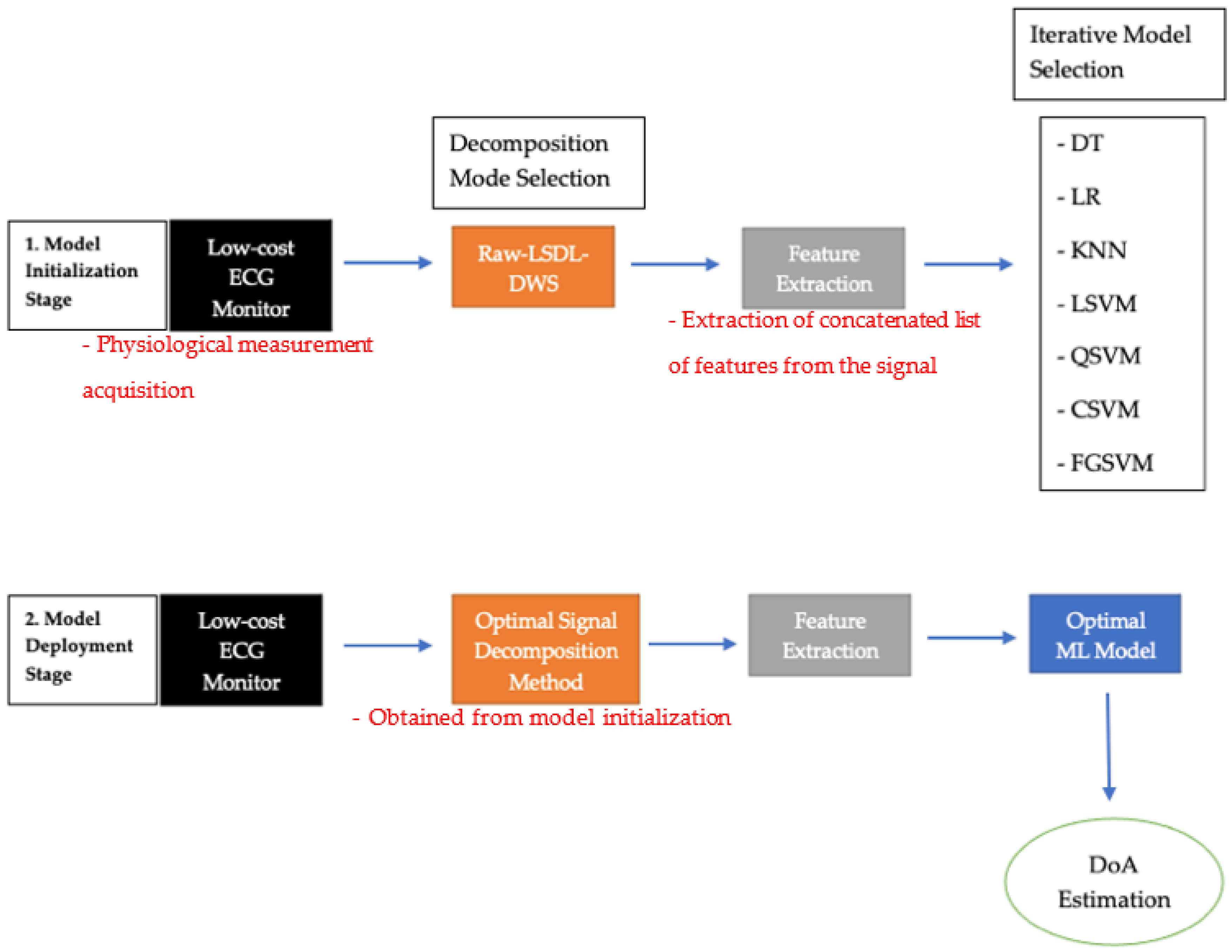
- Investigation of alternative physiological monitors that could contribute towards forming a low-cost avenue towards DoA monitoring by comparing the performance of ECG and EMG monitors with that of the traditionally used EEG;
- -
- Premier use of signal decomposition methods such as the LSDL and DWS for the preprocessing and decomposition of ECG and EMG signals from anesthetized patients, with a view towards enhancing the DoA information that can be decoded and inferred from the signal;
- -
- Comparison of the DoA estimation prowess across multiple classification models of varied model architecture complexities.
2. Materials and Methods
2.1. Dataset and Information
2.2. Physiological Measurement Instrumentations
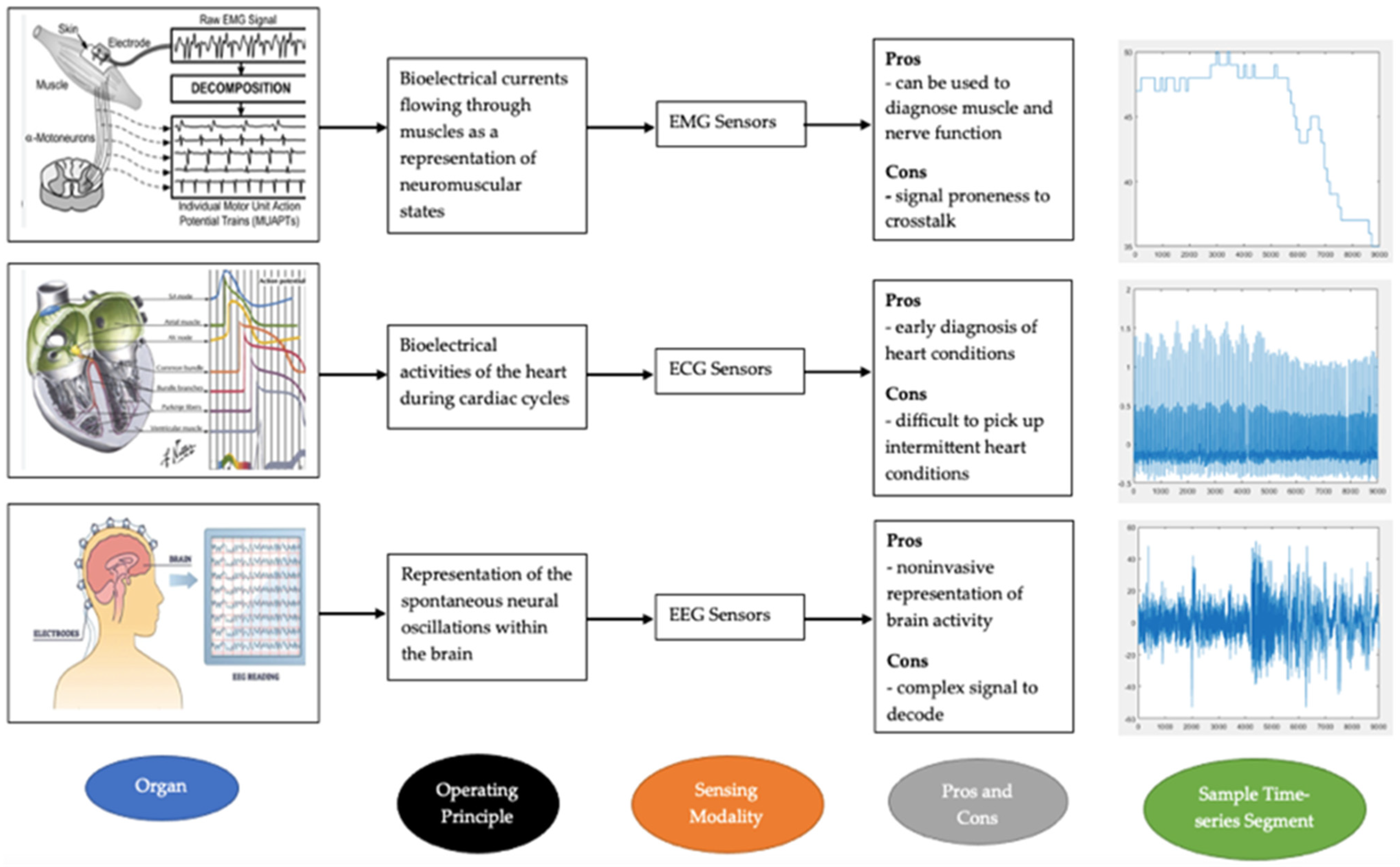
2.2.1. EMG
2.2.2. EEG
2.2.3. ECG
- -
- Heart Tissue
2.3. Signal Decomposition
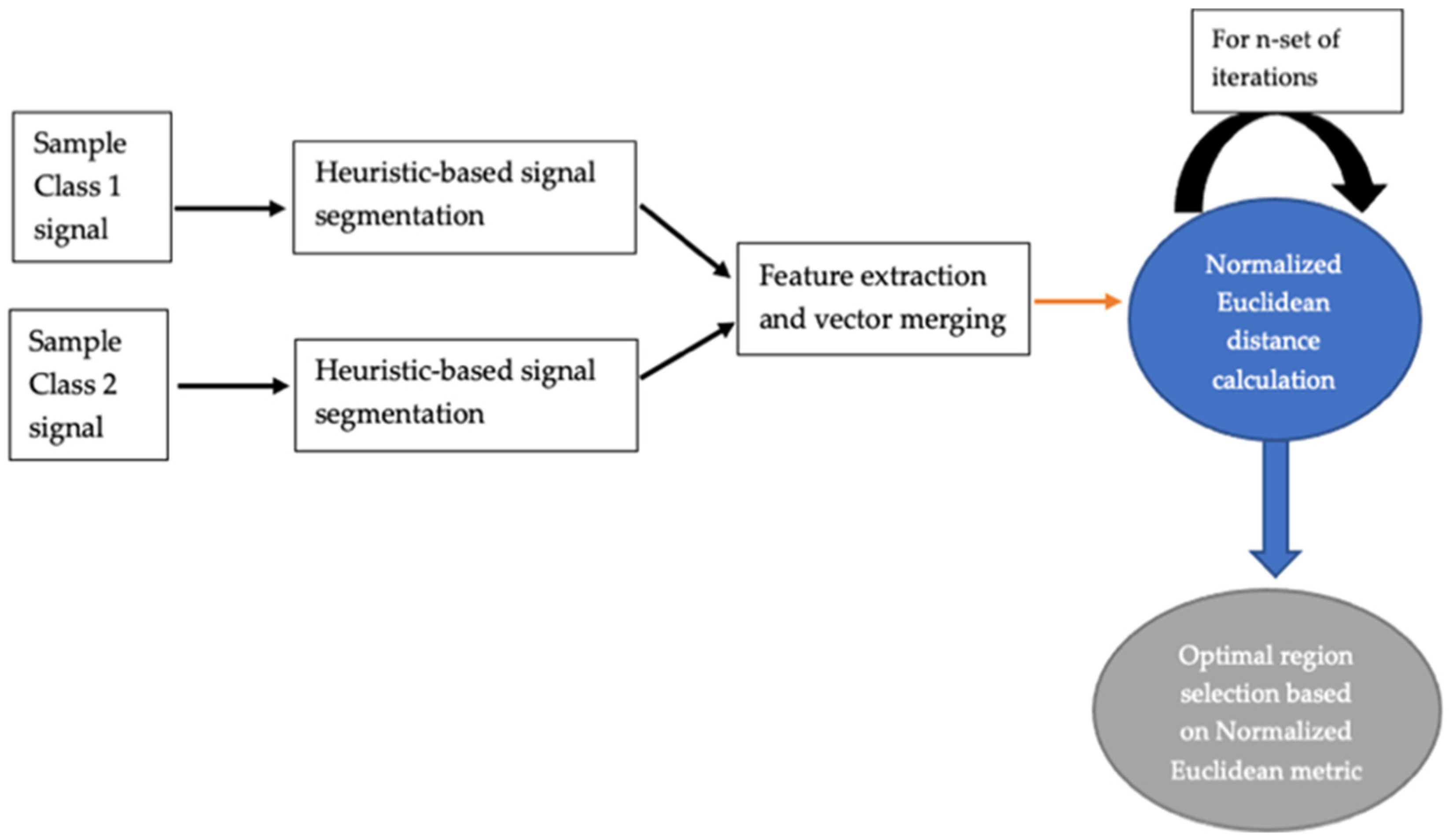
2.3.1. LSDL
2.3.2. Optimal Threshold Search Results
- Case Study 1

| Threshold Region | 1st Iteration | 2nd Iteration | 3rd Iteration |
|---|---|---|---|
| Upper Threshold Region | 2.0026 | 2.0093 | 2.2619 |
| Lower Threshold Region | 2.0000 | 2.0002 | 2.0046 |
| Threshold Region | 1st Iteration | 2nd Iteration | 3rd Iteration |
|---|---|---|---|
| Upper Threshold Region | 2.0092 | 2.0390 | 2.1723 |
| Lower Threshold Region | 2.0212 | 2.0013 | 2.0066 |
- Case Study 2
| Threshold Region | 1st Iteration | 2nd Iteration | 3rd Iteration |
|---|---|---|---|
| Upper Threshold Region | 2.5750 | 2.7190 | 2.8217 |
| Lower Threshold Region | 2.0111 | 2.0020 | 2.0080 |
| Threshold Region | 1st Iteration | 2nd Iteration | 3rd Iteration |
|---|---|---|---|
| Upper Threshold Region | 2.2981 | 2.4454 | 2.4794 |
| Lower Threshold Region | 2.0371 | 2.0654 | 2.1704 |
- Case Study 3
| Threshold Region | 1st Iteration | 2nd Iteration | 3rd Iteration |
|---|---|---|---|
| Upper Threshold Region | 2.7864 | 2.7901 | 2.7996 |
| Lower Threshold Region | 2.7040 | 2.6994 | 2.7071 |
| Threshold Region | 1st Iteration | 2nd Iteration | 3rd Iteration |
|---|---|---|---|
| Upper Threshold Region | 2.5842 | 2.5956 | 2.6032 |
| Lower Threshold Region | 2.2822 | 2.1494 | 2.0004 |
- -
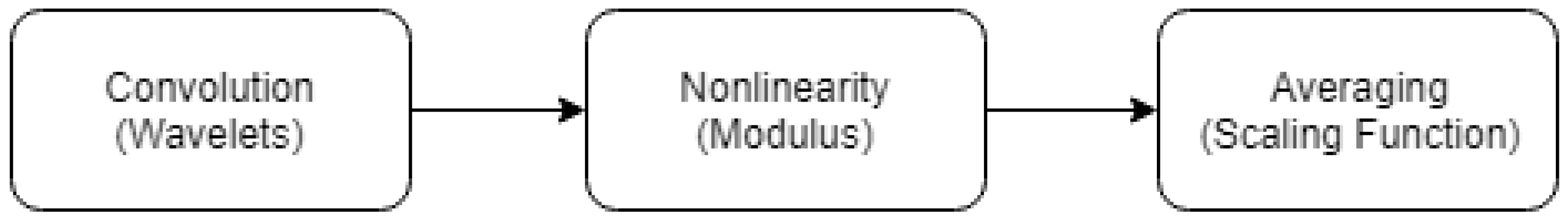
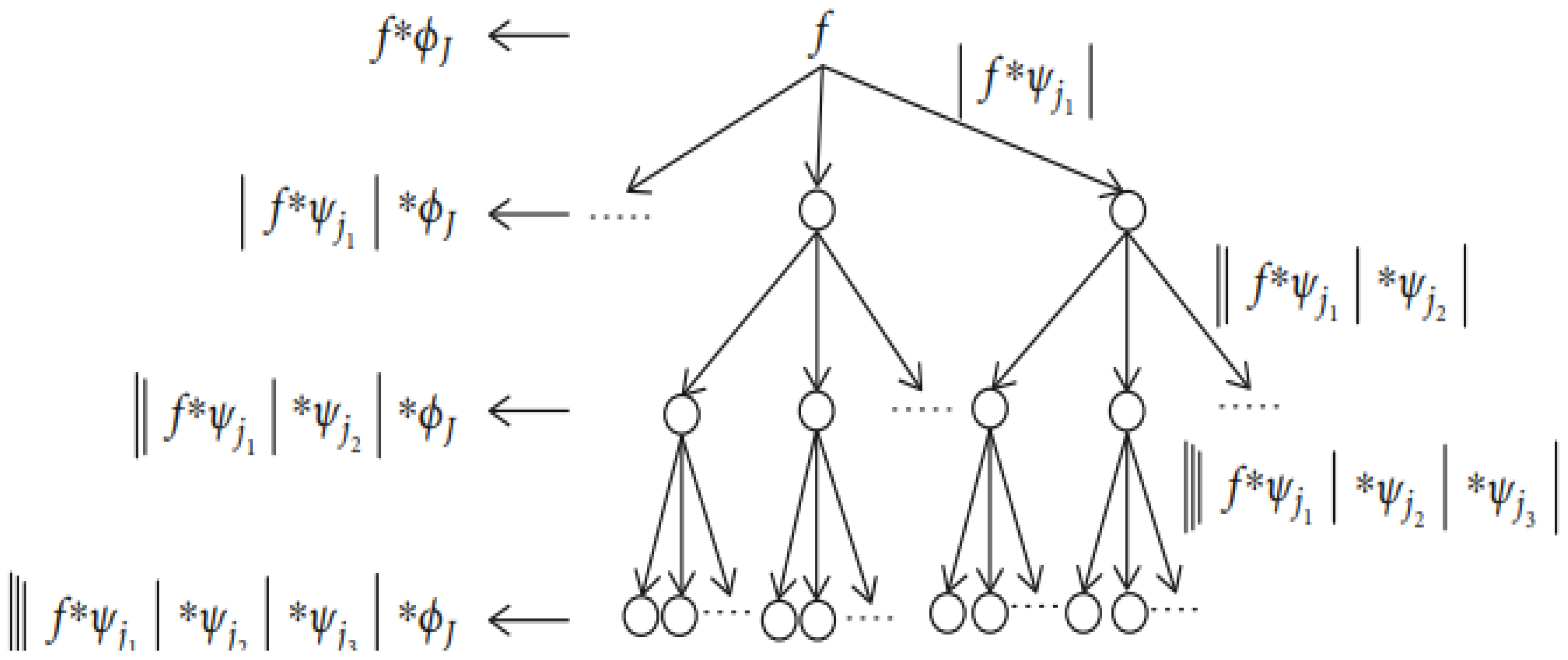
- DWS
2.3.3. Feature Extraction
2.3.4. Machine Learning Models
3. Results and Discussion
3.1. Case Study 1
Classification Problem: BIS over 40 and under 40
3.2. Case Study 2
Classification Problem: BIS over 20 and under 20
3.3. Case Study 3
Classification Problem: BIS over 40 and under 40
4. Conclusions and Future Work
Author Contributions
Funding
Informed Consent Statement
Data Availability Statement
Acknowledgments
Conflicts of Interest
References
- Alwardt, C.M.; Redford, D.; Larson, D.F. General Anesthesia in Cardiac Surgery: A Review of Drugs and Practices. J. Extra Corpor. Technol. 2005, 37, 227–235. [Google Scholar]
- Lan, J.-Y.; Abbod, M.F.; Yeh, R.-G.; Fan, S.-Z.; Shieh, J.-S. Review: Intelligent Modeling and Control in Anesthesia. J. Med. Biol. Eng. 2012, 32, 293–307. [Google Scholar]
- Gruenewald, M.; Ilies, C.; Herz, J.; Schoenherr, T.; Fudickar, A.; Höcker, J.; Bein, B. Influence of Nociceptive Stimulation on Analgesia Nociception Index (ANI) during Propofol-Remifentanil Anaesthesia. Br. J. Anaesth. 2013, 110, 1024–1030. [Google Scholar] [CrossRef]
- Roy Chowdhury, M.; Madanu, R.; Abbod, M.F.; Fan, S.-Z.; Shieh, J.-S. Deep Learning via ECG and PPG Signals for Prediction of Depth of Anesthesia. Biomed. Signal Process. Control 2021, 68, 102663. [Google Scholar] [CrossRef]
- Kissin, I. Depth of Anesthesia and Bispectral Index Monitoring. Anesth. Analg. 2000, 90, 1114–1117. [Google Scholar] [CrossRef] [PubMed]
- Medical Advisory Secretariat. Bispectral Index Monitor: An Evidence-Based Analysis. Ont. Health Technol. Assess. Ser. 2004, 4, 1–70. [Google Scholar]
- Liu, Q.; Chen, Y.-F.; Fan, S.-Z.; Abbod, M.F.; Shieh, J.-S. Quasi-Periodicities Detection Using Phase-Rectified Signal Averaging in EEG Signals as a Depth of Anesthesia Monitor. IEEE Trans. Neural Syst. Rehabil. Eng. 2017, 25, 1773–1784. [Google Scholar] [CrossRef]
- Liu, Q.; Ma, L.; Chiu, R.-C.; Fan, S.-Z.; Abbod, M.F.; Shieh, J.-S. HRV-Derived Data Similarity and Distribution Index Based on Ensemble Neural Network for Measuring Depth of Anaesthesia. PeerJ 2017, 5, e4067. [Google Scholar] [CrossRef]
- Nsugbe, E.; Connelly, S. Multiscale Depth of Anaesthesia Prediction for Surgery Using Frontal Cortex Electroencephalography. Healthc. Technol. Lett. 2022, 9, 43–53. [Google Scholar] [CrossRef] [PubMed]
- Nsugbe, E.; Connelly, S. A Pilot on Intelligence Fusion for Anesthesia Depth Prediction during Surgery Using Frontal Cortex Neural Oscillations. Biomed. Eng. Adv. 2022, 4, 100051. [Google Scholar] [CrossRef]
- Ponde, V. Recent Trends in Paediatric Regional Anaesthesia. Indian J. Anaesth. 2019, 63, 746–753. [Google Scholar] [CrossRef]
- Tyers, M.R.; Russell, W.J.; Runciman, W.B. Electrocardiographic Monitoring in Anaesthesia. Anaesth. Intensive Care 1988, 16, 66–69. [Google Scholar] [CrossRef]
- Iohom, G. Basic Patient Monitoring during Anesthesia—UpToDate. Available online: https://www.uptodate.com/contents/basic-patient-monitoring-during-anesthesia (accessed on 10 June 2023).
- Zhou, Z.-H. Machine Learning; Springer Nature: Berlin, Germany, 2021; ISBN 9789811519673. [Google Scholar]
- Adarsh, S.L.; Venugopal Syam, K.; Philip, L.M.; Martin John, K.D.; Dileepkumar, K.M.; Krathiayini, K.; Ajithkumar, S.; Devanand, C.B. Electrocardiographic Evaluation of Balanced General Anaesthesia in Adult Domestic Cats (Felis Catus). Indian J. Canine Pract. 2022, 14, 22–24. [Google Scholar] [CrossRef]
- Jo, Y.-Y.; Jang, J.-H.; Kwon, J.; Lee, H.-C.; Jung, C.-W.; Byun, S.; Jeong, H.-G. Predicting Intraoperative Hypotension Using Deep Learning with Waveforms of Arterial Blood Pressure, Electroencephalogram, and Electrocardiogram: Retrospective Study. PLoS ONE 2022, 17, e0272055. [Google Scholar] [CrossRef] [PubMed]
- Obert, D.P.; Schweizer, C.; Zinn, S.; Kratzer, S.; Hight, D.; Sleigh, J.; Schneider, G.; García, P.S.; Kreuzer, M. The Influence of Age on EEG-Based Anaesthesia Indices. J. Clin. Anesth. 2021, 73, 110325. [Google Scholar] [CrossRef]
- Zhan, J.; Wu, Z.; Duan, Z.; Yang, G.; Du, Z.; Bao, X.; Li, H. Heart Rate Variability-Derived Features Based on Deep Neural Network for Distinguishing Different Anaesthesia States. BMC Anesthesiol. 2021, 21, 66. [Google Scholar] [CrossRef] [PubMed]
- Orfanidis, S.J. Introduction to Signal Processing; Prentice Hall Signal Processing Series; Prentice Hall: Englewood Cliffs, NJ, USA, 1996; ISBN 978-0-13-209172-5. [Google Scholar]
- Mallat, S.G. A Theory for Multiresolution Signal Decomposition: The Wavelet Representation. IEEE Trans. Pattern Anal. Mach. Intell. 1989, 11, 674–693. [Google Scholar] [CrossRef]
- Stallone, A.; Cicone, A.; Materassi, M. New Insights and Best Practices for the Successful Use of Empirical Mode Decomposition, Iterative Filtering and Derived Algorithms. Sci. Rep. 2020, 10, 15161. [Google Scholar] [CrossRef] [PubMed]
- Soltani, S. On the Use of the Wavelet Decomposition for Time Series Prediction. Neurocomputing 2002, 48, 267–277. [Google Scholar] [CrossRef]
- Kavakiotis, I.; Tsave, O.; Salifoglou, A.; Maglaveras, N.; Vlahavas, I.; Chouvarda, I. Machine Learning and Data Mining Methods in Diabetes Research. Comput. Struct. Biotechnol. J. 2017, 15, 104–116. [Google Scholar] [CrossRef]
- Nsugbe, E. Enhanced Recognition of Adolescents with Schizophrenia and a Computational Contrast of Their Neuroanatomy with Healthy Patients Using Brainwave Signals. Appl. AI Lett. 2023, 4, e79. [Google Scholar] [CrossRef]
- Nsugbe, E.; Ser, H.-L.; Ong, H.-F.; Ming, L.C.; Goh, K.-W.; Goh, B.-H.; Lee, W.-L. On an Affordable Approach towards the Diagnosis and Care for Prostate Cancer Patients Using Urine, FTIR and Prediction Machines. Diagnostics 2022, 12, 2099. [Google Scholar] [CrossRef] [PubMed]
- Nsugbe, E. Towards the Use of Cybernetics for an Enhanced Cervical Cancer Care Strategy. Intell. Med. 2022, 2, 117–126. [Google Scholar] [CrossRef]
- Liu, D.; Görges, M.; Jenkins, S.A. University of Queensland Vital Signs Dataset: Development of an Accessible Repository of Anesthesia Patient Monitoring Data for Research. Anesth. Analg. 2012, 114, 584–589. [Google Scholar] [CrossRef]
- Rodriguez-Falces, J.; Navallas, J.; Malanda, A. Computational Intelligence in Electromyography Analysis—A Perspective on Current Applications and Future Challenges. In Computational Intelligence in Electromyography Analysis—A Perspective on Current Applications and Future Challenges; Naik, G.R., Ed.; IntechOpen: London, UK, 2012; ISBN 978-953-51-0805-4. [Google Scholar]
- Cram, J.R.; Kasman, G.S.; Holtz, J. Introduction to Surface Electromyography; Aspen Publishers: Gaithersburg, MD, USA, 1998; ISBN 978-0-8342-0751-6. [Google Scholar]
- Petersen, E.; Rostalski, P. A Comprehensive Mathematical Model of Motor Unit Pool Organization, Surface Electromyography, and Force Generation. Front. Physiol. 2019, 10, 176. [Google Scholar] [CrossRef]
- Nsugbe, E.; Samuel, O.W.; Asogbon, M.G.; Li, G. Phantom Motion Intent Decoding for Transhumeral Prosthesis Control with Fused Neuromuscular and Brain Wave Signals. IET Cyber-Syst. Robot. 2021, 3, 77–88. [Google Scholar] [CrossRef]
- Darbas, M.; Lohrengel, S. Review on Mathematical Modelling of Electroencephalography (EEG). Jahresber. Dtsch. Math. Ver. 2019, 121, 3–39. [Google Scholar] [CrossRef]
- Doschoris, M.; Kariotou, F. Mathematical Foundation of Electroencephalography. In Electroencephalography; Sittiprapaporn, P., Ed.; IntechOpen: London, UK, 2017; ISBN 978-953-51-3638-5. [Google Scholar]
- Boulakia, M.; Cazeau, S.; Fernández, M.A.; Gerbeau, J.-F.; Zemzemi, N. Mathematical Modeling of Electrocardiograms: A Numerical Study. Ann. Biomed. Eng. 2010, 38, 1071–1097. [Google Scholar] [CrossRef]
- Pullan, A.J.; Cheng, L.K.; Buist, M.L. Mathematically Modelling the Electrical Activity of the Heart: From Cell to Body Surface and Back Again; World Scientific: Hackensack, NJ, USA, 2005; ISBN 978-981-256-373-6. [Google Scholar]
- Sundnes, J.; Lines, G.; Cai, X.; Nielsen, B.F.; Mardal, K.-A.; Tveito, A. Computing the Electrical Activity in the Heart; Springer: Berlin/Heidelberg, Germany, 2006; ISBN 978-3-540-33432-3. [Google Scholar]
- Tung, L. A Bi-Domain Model for Describing Ischemic Myocardial d-c Potentials. Ph.D. Thesis, Massachusetts Institute of Technology, Cambridge, MA, USA, 1978. [Google Scholar]
- De Luca, C.J.; Adam, A.; Wotiz, R.; Gilmore, L.D.; Nawab, S.H. Decomposition of Surface EMG Signals. J. Neurophysiol. 2006, 96, 1646–1657. [Google Scholar] [CrossRef]
- Sarazan, R.D. The QT Interval of the Electrocardiogram. In Encyclopedia of Toxicology, 3rd ed.; Wexler, P., Ed.; Academic Press: Oxford, UK, 2014; pp. 10–15. ISBN 978-0-12-386455-0. [Google Scholar]
- Eeg and Brainwaves. Bright Brain—London’s Eeg, Neurofeedback and Brain Stimulation Centre. Available online: https://www.brightbraincentre.co.uk/electroencephalogram-eeg-brainwaves/ (accessed on 29 August 2023).
- Durak, L.; Arikan, O. Short-Time Fourier Transform: Two Fundamental Properties and an Optimal Implementation. IEEE Trans. Signal Process. 2003, 51, 1231–1242. [Google Scholar] [CrossRef]
- Klimesch, W. The Frequency Architecture of Brain and Brain Body Oscillations: An Analysis. Eur. J. Neurosci. 2018, 48, 2431–2453. [Google Scholar] [CrossRef] [PubMed]
- Nsugbe, E.; Starr, A.; Ruiz-Carcel, C. Monitoring the Particle Size Distribution of a Powder Mixing Process with Acoustic Emissions: A Review. Eng. Technol. Ref. 2016, 1–12. [Google Scholar] [CrossRef]
- Nsugbe, E. Particle Size Distribution Estimation of a Powder Agglomeration Process Using Acoustic Emissions. Ph.D. Thesis, Cranfield University, Cranfield, UK, 2017. [Google Scholar]
- Nsugbe, E.; Starr, A.; Jennions, I.; Ruiz-Carcel, C. Estimation of Online Particle Size Distribution of a Particle Mixture in Free Fall with Acoustic Emission. Part. Sci. Technol. 2019, 37, 953–963. [Google Scholar] [CrossRef]
- Nsugbe, E.; Williams Samuel, O.; Asogbon, M.G.; Li, G. Contrast of Multi-Resolution Analysis Approach to Transhumeral Phantom Motion Decoding. CAAI Trans. Intell. Technol. 2021, 6, 360–375. [Google Scholar] [CrossRef]
- Nsugbe, E.; Sanusi, I. Towards an Affordable Magnetomyography Instrumentation and Low Model Complexity Approach for Labour Imminency Prediction Using a Novel Multiresolution Analysis. Appl. AI Lett. 2021, 2, e34. [Google Scholar] [CrossRef]
- Nsugbe, E. On the Use of Spectroscopy, Prediction Machines and Cybernetics for an Affordable and Proactive Care Approach for Endometrial Cancer. Biomed. Eng. Adv. 2022, 4, 100057. [Google Scholar] [CrossRef]
- Gower, J.C. Properties of Euclidean and Non-Euclidean Distance Matrices. Linear Algebra Its Appl. 1985, 67, 81–97. [Google Scholar] [CrossRef]
- Wavelet Scattering. Available online: https://uk.mathworks.com/help/wavelet/ug/wavelet-scattering.html (accessed on 29 August 2023).
- Mallat, S. Group Invariant Scattering. Commun. Pure Appl. Math. 2012, 65, 1331–1398. [Google Scholar] [CrossRef]
- Bruna, J.; Mallat, S. Invariant Scattering Convolution Networks. IEEE Trans. Pattern Anal. Mach. Intell. 2013, 35, 1872–1886. [Google Scholar] [CrossRef]
- Liu, Z.; Yao, G.; Zhang, Q.; Zhang, J.; Zeng, X. Wavelet Scattering Transform for ECG Beat Classification. Comput. Math. Methods Med. 2020, 2020, e3215681. [Google Scholar] [CrossRef] [PubMed]
- Nsugbe, E. On the Application of Metaheuristics and Deep Wavelet Scattering Decompositions for the Prediction of Adolescent Psychosis Using EEG Brain Wave Signals. Digit. Technol. Res. Appl. 2022, 1, 9–24. [Google Scholar] [CrossRef]
- Charbuty, B.; Abdulazeez, A. Classification Based on Decision Tree Algorithm for Machine Learning. J. Appl. Sci. Technol. Trends 2021, 2, 20–28. [Google Scholar] [CrossRef]
- LaValley, M.P. Logistic Regression. Circulation 2008, 117, 2395–2399. [Google Scholar] [CrossRef] [PubMed]
- Kramer, O. K-Nearest Neighbors. In Dimensionality Reduction with Unsupervised Nearest Neighbors; Intelligent Systems Reference Library; Springer: Berlin/Heidelberg, Germany, 2013; Volume 51, pp. 13–23. ISBN 978-3-642-38651-0. [Google Scholar]
- Noble, W.S. What Is a Support Vector Machine? Nat. Biotechnol. 2006, 24, 1565–1567. [Google Scholar] [CrossRef]


| Case Study | Signal Windowing | Classification Exercise | Total Time Utilized (Minutes) |
|---|---|---|---|
| Case 1 | 9000 samples × 19 (for all modalities) | BIS Over 40 and Under 40 | 28.5 |
| Case 2 | 6000 samples × 19 (for all modalities) | BIS Over 20 and Under 20 | 19 |
| Case 3 | 9000 samples × 19 (for all modalities) | BIS Over 40 and Under 40 | 28.5 |
| Machine Learning Model | Raw EMG Accuracy (%) | Raw ECG Accuracy (%) | Raw EEG Accuracy (%) | Raw EMG-ECG-EEG Accuracy (%) |
|---|---|---|---|---|
| Decision Tree | 44.7 | 52.6 | 65.8 | 31.6 |
| Logistic Regression | 42.1 | 47.4 | 44.7 | 34.2 |
| K-Nearest Neighbor | 47.4 | 52.6 | 47.4 | 47.4 |
| Linear Support Vector Machine | 34.2 | 36.8 | 76.3 | 57.9 |
| Quadratic Support Vector Machine | 52.6 | 52.6 | 50.0 | 57.9 |
| Cubic Support Vector Machine | 44.7 | 34.2 | 65.8 | 60.5 |
| Fine Gaussian Support Vector Machine | 42.1 | 50.0 | 57.9 | 50.0 |
| Machine Learning Model | LSDL ECG Accuracy (%) | LSDL EEG Accuracy (%) |
|---|---|---|
| Decision Tree | 55.3 | 60.5 |
| Logistic Regression | 89.5 | 86.8 |
| K-Nearest Neighbor | 47.4 | 76.3 |
| Linear Support Vector Machine | 44.7 | 73.7 |
| Quadratic Support Vector Machine | 44.7 | 78.9 |
| Cubic Support Vector Machine | 47.4 | 76.3 |
| Fine Gaussian Support Vector Machine | 26.3 | 65.8 |
| Machine Learning Model | DWS EMG Accuracy (%) | DWS ECG Accuracy (%) | DWS EEG Accuracy (%) |
|---|---|---|---|
| Decision Tree | 67.8 | 74.9 | 66.9 |
| Logistic Regression | 61.2 | 76.2 | 70.5 |
| K-Nearest Neighbor | 66.3 | 88.6 | 98.0 |
| Linear Support Vector Machine | 58.9 | 74.2 | 69.1 |
| Quadratic Support Vector Machine | 53.3 | 88.5 | 87.4 |
| Cubic Support Vector Machine | 51.8 | 90.8 | 94.7 |
| Fine Gaussian Support Vector Machine | 59.5 | 84.2 | 85.8 |
| Best Modality | Best Prediction Accuracy (%) |
|---|---|
| EMG | DWS DT: 67.8 |
| ECG | DWS CSVM: 90.8 |
| EEG | DWS KNN: 98.0 |
| Machine Learning Model | Raw EMG Accuracy (%) | Raw ECG Accuracy (%) | Raw EEG Accuracy (%) | Raw EMG-ECG-EEG Accuracy (%) |
|---|---|---|---|---|
| Decision Tree | 84.2 | 71.1 | 81.6 | 84.2 |
| Logistic Regression | 50.0 | 71.1 | 73.7 | 63.2 |
| K-Nearest Neighbor | 52.6 | 47.4 | 47.4 | 47.4 |
| Linear Support Vector Machine | 50.0 | 76.3 | 73.7 | 78.9 |
| Quadratic Support Vector Machine | 50.0 | 81.6 | 78.9 | 78.9 |
| Cubic Support Vector Machine | 50.0 | 78.9 | 81.6 | 78.9 |
| Fine Gaussian Support Vector Machine | 50.0 | 73.7 | 71.1 | 47.4 |
| Machine Learning Model | LSDL ECG Accuracy (%) | LSDL EEG Accuracy (%) |
|---|---|---|
| Decision Tree | 44.7 | 52.6 |
| Logistic Regression | 81.6 | 78.9 |
| K-Nearest Neighbor | 65.8 | 39.5 |
| Linear Support Vector Machine | 47.4 | 52.6 |
| Quadratic Support Vector Machine | 63.2 | 55.3 |
| Cubic Support Vector Machine | 65.8 | 65.8 |
| Fine Gaussian Support Vector Machine | 50.0 | 44.7 |
| Machine Learning Model | DWS EMG Accuracy (%) | DWS ECG Accuracy (%) | DWS EEG Accuracy (%) |
|---|---|---|---|
| Decision Tree | 85.7 | 96.5 | 90.6 |
| Logistic Regression | 73.7 | 98.8 | 93.0 |
| K-Nearest Neighbor | 87.4 | 98.8 | 98.0 |
| Linear Support Vector Machine | 89.8 | 95.9 | 93.6 |
| Quadratic Support Vector Machine | 88.6 | 99.4 | 97.7 |
| Cubic Support Vector Machine | 88.6 | 99.7 | 98.5 |
| Fine Gaussian Support Vector Machine | 86.8 | 95.9 | 84.8 |
| Best Modality | Best Prediction Accuracy (%) |
|---|---|
| Best EMG | DWS LSVM: 89.8 |
| Best ECG | DWS CSVM: 99.7 |
| Best EEG | DWS CSVM: 98.5 |
| Machine Learning Model | Raw EMG Accuracy (%) | Raw ECG Accuracy (%) | Raw EEG Accuracy (%) | Raw EMG-ECG-EEG Accuracy (%) |
|---|---|---|---|---|
| Decision Tree | 42.1 | 71.1 | 60.5 | 52.6 |
| Logistic Regression | 42.1 | 52.6 | 60.5 | 55.3 |
| K-Nearest Neighbor | 42.1 | 60.5 | 63.2 | 76.3 |
| Linear Support Vector Machine | 55.3 | 42.1 | 57.9 | 50.0 |
| Quadratic Support Vector Machine | 47.4 | 47.4 | 68.4 | 71.1 |
| Cubic Support Vector Machine | 47.4 | 50.0 | 71.1 | 76.3 |
| Fine Gaussian Support Vector Machine | 52.6 | 52.6 | 65.8 | 63.2 |
| Machine Learning Model | LSDL ECG Accuracy (%) | LSDL EEG Accuracy (%) |
|---|---|---|
| Decision Tree | 94.7 | 97.4 |
| Logistic Regression | 94.7 | 100 |
| K-Nearest Neighbor | 89.5 | 100 |
| Linear Support Vector Machine | 94.7 | 100 |
| Quadratic Support Vector Machine | 94.7 | 100 |
| Cubic Support Vector Machine | 92.1 | 100 |
| Fine Gaussian Support Vector Machine | 84.2 | 92.1 |
| Machine Learning Model | DWS EMG Accuracy (%) | DWS ECG Accuracy (%) | DWS EEG Accuracy (%) |
|---|---|---|---|
| Decision Tree | 64.0 | 72.3 | 68.0 |
| Logistic Regression | 57.1 | 75.7 | 71.7 |
| K-Nearest Neighbor | 63.4 | 89.1 | 98.5 |
| Linear Support Vector Machine | 56.8 | 76.5 | 69.8 |
| Quadratic Support Vector Machine | 51.2 | 87.9 | 87.6 |
| Cubic Support Vector Machine | 50.4 | 50.2 | 95.1 |
| Fine Gaussian Support Vector Machine | 59.9 | 77.9 | 89.5 |
| Best Modality | Best Prediction Accuracy (%) |
|---|---|
| Best EMG | DWS DT: 64.0 |
| Best ECG | LSDL Logistic Regression: 94.7 |
| Best EEG | LSDL Logistic Regression: 100 |
Disclaimer/Publisher’s Note: The statements, opinions and data contained in all publications are solely those of the individual author(s) and contributor(s) and not of MDPI and/or the editor(s). MDPI and/or the editor(s) disclaim responsibility for any injury to people or property resulting from any ideas, methods, instructions or products referred to in the content. |
© 2023 by the authors. Licensee MDPI, Basel, Switzerland. This article is an open access article distributed under the terms and conditions of the Creative Commons Attribution (CC BY) license (https://creativecommons.org/licenses/by/4.0/).
Share and Cite
Nsugbe, E.; Connelly, S.; Mutanga, I. Towards an Affordable Means of Surgical Depth of Anesthesia Monitoring: An EMG-ECG-EEG Case Study. BioMedInformatics 2023, 3, 769-790. https://doi.org/10.3390/biomedinformatics3030049
Nsugbe E, Connelly S, Mutanga I. Towards an Affordable Means of Surgical Depth of Anesthesia Monitoring: An EMG-ECG-EEG Case Study. BioMedInformatics. 2023; 3(3):769-790. https://doi.org/10.3390/biomedinformatics3030049
Chicago/Turabian StyleNsugbe, Ejay, Stephanie Connelly, and Ian Mutanga. 2023. "Towards an Affordable Means of Surgical Depth of Anesthesia Monitoring: An EMG-ECG-EEG Case Study" BioMedInformatics 3, no. 3: 769-790. https://doi.org/10.3390/biomedinformatics3030049