Article

Evaluating Land Surface Temperature Trends and Explanatory Variables in the Miami Metropolitan Area from 2002–2021

Department of Geosciences, Florida Atlantic University, Boca Raton, FL 33431, USA
*
Author to whom correspondence should be addressed.
Geomatics 2024, 4(1), 1-16; https://doi.org/10.3390/geomatics4010001
Submission received: 29 October 2023 / Revised: 9 December 2023 / Accepted: 23 December 2023 / Published: 25 December 2023

Abstract

:
Physical and climatic variables such as Tree Canopy coverage, Normalized Difference Vegetation Index (NDVI), Distance to Roads, Distance to the Coast, Impervious Surface, and Precipitation can affect land surface temperature (LST). This paper examines the relationships using linear regression models and explores LST trends in the Miami Statistical Area (MSA) between 2002 and 2021. This study evaluates the effect of dry and wet seasons as well as day and night data on LST. A multiscale investigation is used to examine LST trends at the MSA scale, the individual county level, and at the pixel level to provide a detailed local perspective. The multiscale results are needed to understand spatiotemporal LST distributions to plan mitigation measures such as planting trees or greenery to regulate temperature and reduce the impacts of surface urban heat islands. The results indicate that LST values are rising in the MSA with a positive trend throughout the 20-year study period. The rate of change (RoC) for the wet season is smaller than for the dry season. The pixel-level analysis suggests that the RoC is primarily in rural areas and less apparent in urban areas. New development in rural areas may trigger increased RoC. This RoC relates to LST in the MSA and is different from global or regional RoC using air temperature. Results also suggest that climatic explanatory variables have different impacts during the night than they do in the daytime. For instance, the Tree Canopy variable has a positive coefficient, while during the day, the Tree Canopy variable has a negative relationship with LST. The Distance to the Coast variable changes from day to night as well. The increased granularity achieved with the multiscale analysis provides critical information needed to improve the effectiveness of potential mitigation efforts.

1. Introduction

Surface urban heat islands (SUHI) are urbanized areas that experience higher temperatures than rural areas at the surface level [1]. SUHI are identified by the measurements of land surface temperature (LST) and the spatial variation of temperature that covers a large surface area [2]. A SUHI effect occurs when there is an upsurge of human activities and an expansion of densely built environments that result in temperature differences between urban and rural areas [3]. SUHI can occur when buildings and pavement exist instead of vegetation and tree canopies causing anthropogenic heat release [4]. Construction material such as concrete and asphalt used in urban areas does not allow water to stick to the soil causing LST to rise [5]. With the population in urban areas growing, it is estimated that 66% of the total population will be living in urban areas by 2050 [6] and as a result, issues relating to urban heat are becoming more important. SUHI are characterized by the highest intensity of temperature during nights because the air is stagnant while the surface LST reaches the maximum temperature of heat release in the afternoon when sunlight is absorbed [7].
Previous SUHI studies have been conducted in several locations around the world including India [8,9] and China [10,11,12] as well as in selected locations in the United States such as Baltimore [4] and Texas [13]. Bera et al. [8] focuses on LST trends in four megacities in India. The study applies a multiscale analysis and investigates LST trends at a localized scale as well as at the pixel level with a diurnal aspect. Wang et al. [14] investigates LST trends with a multiscale study at the global and pixel levels. The LST trends at the global and pixel scales suggest that the rate of change (RoC) varies among locations. Verbesselt et al. [15] uses local view as well as time series perspectives with annual and seasonal results to explore trends. In diverse environments, the spatiotemporal LST trends can clarify how LST affects small areas of urban environments given the trend’s intensity [8].
The diurnal LST range is an important indicator of global climate change [15]. Diurnal LST provides an understanding of LST trends and how they are affected by physical and climatic explanatory variables [16]. In diverse urban areas, it clarifies how LST affects small units of urban environments and the magnitude of trends [8]. There are many physical and climatic factors that affect LST, and it is important to explore the quantitative relationships between explanatory factors and LST [8]. Previous studies tested explanatory variables such as Normalized Difference Vegetation Index (NDVI) [17], Normalized Difference Building Index (NDBI) [7,15], and Distance to Water [13]. Chen et al. [18] reports that NDVI is negatively correlated with LST causing LST to fall as NDVI increases. Dissanayake et al. [2] finds that NDBI is positively correlated with LST causing LST to increase as NDBI increases. Liu et al. [13] concludes that during the nighttime, LST increases in areas closer to the coast.
Impervious surfaces, roads, and other types of infrastructures in urban settings increase radiation absorption and heat storage in urban areas which can lead to high LST [19]. Impervious surfaces are nonporous land covers that keep water from entering the layers such as buildings, roads, or any type of pavement [20]. Planners in urban areas are trying to limit factors such as impervious surfaces and add greenery to reduce LST. Previous research has shown changes in LST can alter the material and energy balance of the ground and atmosphere which causes changes to important ecological variables such as temperature, precipitation, and vegetation [21]. Increasing vegetation in urban areas as well as tree canopies are recognized as an effective way to mitigate urban heat and to advance adaptation [19].
There has been limited research on South Florida UHI and LST. Previous studies do not take a multiscale examination of LST which encompasses analyzing datasets at three separate scales. In addition, they do not divide South Florida areas by county or investigate it by pixel view. Furthermore, studies in South Florida do not examine seasonal or diurnal LSTs. The current study not only takes a three-level multiscale view of Florida but investigates LST for wet and dry seasons. It also uses the distance to the coastline as an important explanatory factor for LST. Alhawiti et al. [7] study a localized view focusing on Fort Lauderdale. Their study investigates Fort Lauderdale LST for four different months in 2014: March, April, October, and November. Kandel et al. [22] focus on the entire study area in South Florida without dividing it by county or section. Their research focuses on meteorological factors as well as land cover to urban heat with no specific time of diurnal or seasonal evaluations.
There are still gaps in the research relating to LST that need to be addressed, even with the rich literature discussed above. This paper fills some of the gaps by applying a three-level multiscale view in South Florida. This kind of analysis can help advance understanding of which specific places in the study area are most vulnerable. This study undertakes a multiscale investigation of the Miami Statistical Area (MSA) that includes analysis at the MSA level as well as at the county level for Miami-Dade (MDC), Broward (BC), and Palm Beach (PBC) counties, and a pixel-level assessment. Analysis at the pixel level provides a detailed local perspective on the RoC and LST trends while analysis at the MSA level gives a regional perspective, and assessments at the county level provide a comparison among trends of the three counties. A multiscale analysis of LST explanatory factors at the MSA and county levels provides a detailed and diverse understanding of the relationships between the explanatory factors and LST. An examination of trends requires a multiscale approach to enrich our perspective on trends and patterns that may affect the future. The results from this study, the first three-level multiscale effort in South Florida to examine LST trends and explanatory factors, are needed to understand the spatiotemporal distributions of LST to plan mitigation measures such as planting trees or greenery to regulate temperature.
In response to the research gaps, the specific objectives of this study are to: (1) analyze the spatiotemporal patterns of LST and identify the warm and cool areas within the MSA; (2) assess LST trends over the last 20 years (2002–2021) at the MSA, county, and pixel levels; and (3) determine the impacts of physical and environmental factors on LST in different scales. The results will provide spatial information on where mitigation can be most effective in reducing the impacts of SUHI by adding greenery and reducing pavement and buildings.

2. Materials and Methods
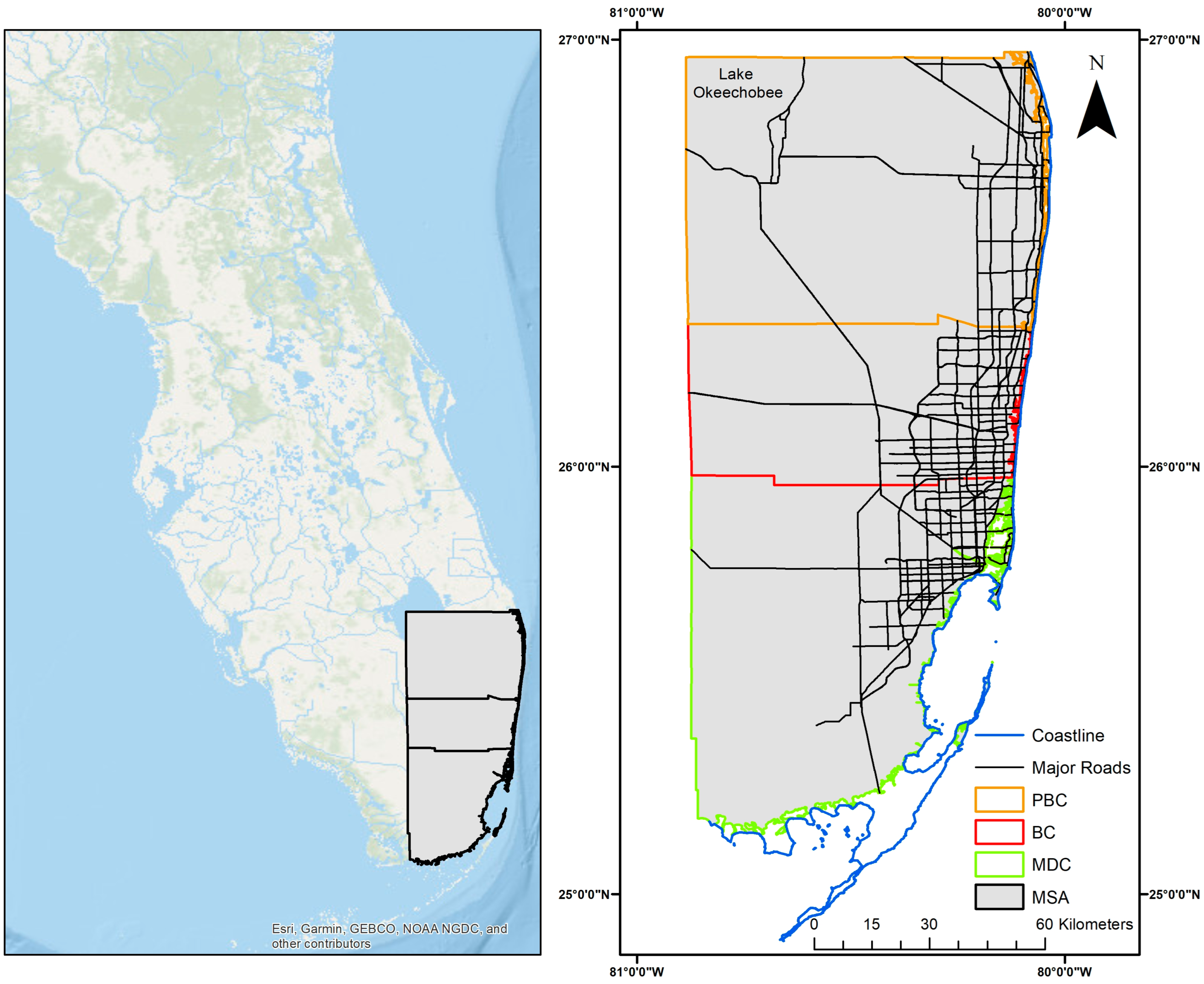
2.1. Study Area

The study area is comprised of the three counties that make up South Florida: PBC, BC, and MDC, commonly known as the MSA, as Figure 1 shows. The MSA was selected because it is the most populous region in Florida, adjacent to the southeastern coast, and has a diversity of land areas including wetlands, agricultural, and urban areas. The urban areas in the MSA are situated along the coastline starting from PBC with West Palm Beach and Boca Raton. BC includes Fort Lauderdale. MDC includes Miami. Urban areas are defined as a built-up area with a population of 50,000 or more [23]. The MSA is located along the Atlantic Ocean and includes Lake Okeechobee and parts of Everglades National Park. South Florida has a subtropical climate characterized by two seasons: the wet season and the dry season. The wet season occurs from May to November and the dry season occurs from November to May. The wet season has hot and humid conditions as well as frequent thunderstorms while the dry season has cooler temperatures with lower humidity and less thunderstorms and precipitation [24].
The MSA has a land area of 13,123 km2 and had a population of 6,091,747 in 2021 [25] Florida is the fastest growing state in population with an increase of 1.9% between the years 2021 and 2022 [25]. Florida’s population increased from 12 million in 1990 to approximately 21 million in 2018 with noticeable expansion in South Florida’s urban region [6]. PBC is the largest county in Florida with land area at 6677 km2. The MSA also has the largest lake in Florida, Lake Okeechobee, which is in PBC.

2.2. Data

2.2.1. LST Data

The Moderate Resolution Imaging Spectroradiometer (MODIS) is an Earth Observing System that serves as an important source for global studies of atmosphere, land, and ocean processes [26]. MODIS is aboard the Terra and Aqua satellites [27] and has 36 spectral bands providing global coverage every 1 to 2 days during the day and night [28]. The LST data were accessed using the Google Earth Engine (GEE) which is a popular cloud computing system for geospatial analytics providing users access to a wide web-based set of data [29]. GEE offers user access and processing of data from the public or private catalogs accelerating scientific discovery [30]. Through GEE, MODIS product, MOD11A1.061 Terra LST and Emissivity Daily, global images were accessed in 1 km spatial resolution from the National Aeronautics and Space Administration (NASA) Land Processes Distributed Active Archive Center at the United States Geological Survey (USGS) Earth Resources Observation and Science Center. The MOD11A1 data are available from the year 2000 to the present on GEE. This study used 20 years of MOD11A1 data from 2002 through 2021. The mean LST was determined by filtering out the wet season and dry season. Filtering was implemented by using the months for each season such as November to April for the dry season and May to October for the wet season. The LST data were further separated by Dry Day LST, Dry Night LST, Wet Day LST, and Wet Night LST. The LST was converted to degrees Celsius from its original Kelvin.
Figure 1. The study area is the Miami metropolitan area.
Geomatics 04 00001 g001

2.2.2. Major Explanatory Variables of LST
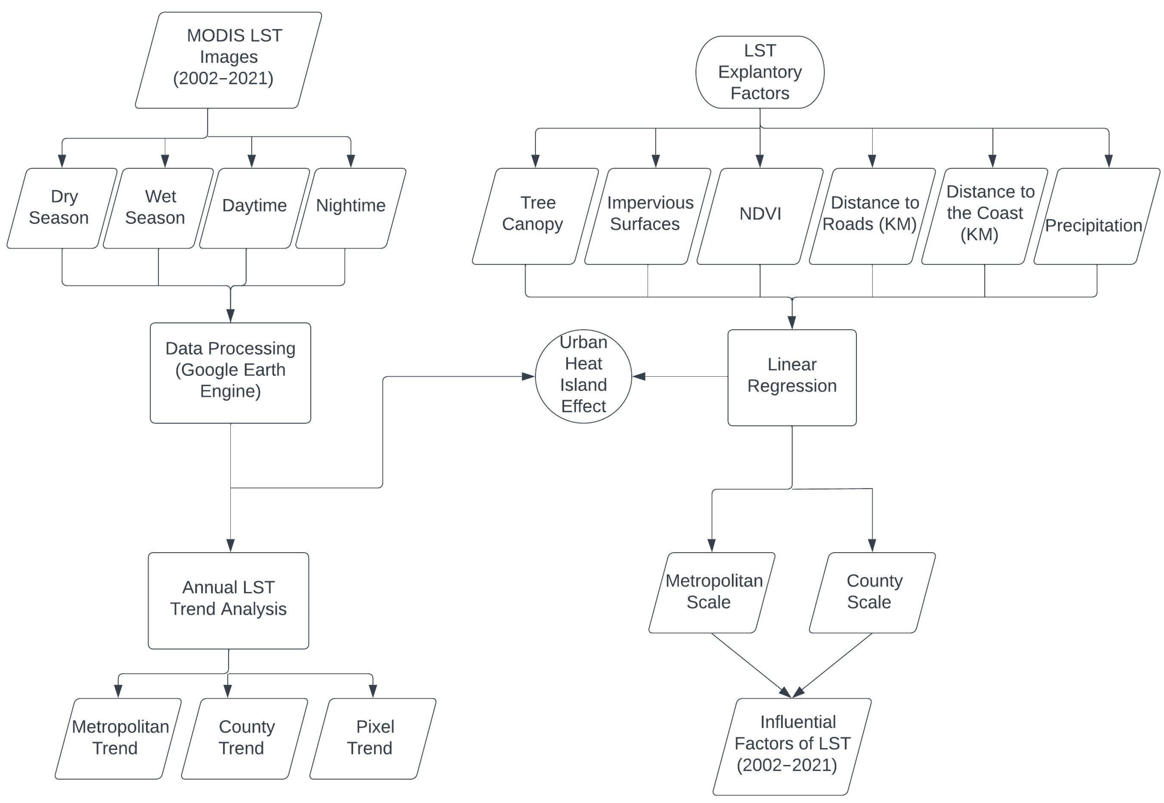
Although there are many factors affecting LST, the six physical and climatic explanatory variables included in the study were selected based on results from previous studies and hypotheses on the expected impacts of the variables on LST. These explanatory variables contain physical and climatic information from remote sensing imagery [8]. The physical variables include Tree Canopy, Impervious Surfaces, NDVI, Distance to Roads, and Distance to the Coast. Distance to Roads was selected based on previous studies by Feng et al. [31] and the hypothesis that traffic and road pavement increase LST with a positive impact on creating SUHI. Precipitation is the key climatic variable used. Distance to the Coast and Precipitation were selected because of characteristics in the South Florida study area. This area has a significant amount of coastline as well as a large amount of precipitation, both of which are expected to reduce LST with a negative impact on the creation of SUHI. Table 1 shows the explanatory variables used in this study.
The NDVI data are widely used in urban climate studies especially when detecting vegetation coverage. NDVI ranges from −1 to 1, with higher positive numbers suggesting dense vegetation and lower values indicating developed urban areas [2]. Tree Canopy data were hypothesized to have an important impact on LST with greater amounts of greenery resulting in cooler areas. Trees cool the surrounding environment by transpiration in which the water is taken up by the tree roots and moved through the stem which eventually evaporates from the leaves [32]. A tree canopy is known as woody vegetation with forests of branches and trees [33]. Heat trapped under a dense tree canopy is due to restricted longwave radiative cooling and leads to elevated nighttime temperatures [34]. Vegetation coverage can change the radiative and non-radiative properties of the surface. Surface energy balance processes can vary spatially and seasonally, which can affect LST depending on the vegetation coverage and type [35].
Impervious Surface is one of the most important land cover types dealing with urban climate by the altering sensible and latent heat fluxes within urban surfaces [36]. Surface energy balance theory is relevant to understanding how the amount of available radiation and energy can impact LST of impervious surfaces. Surface energy balance describes the amount of energy flex that is available to evaporate surface water which affects LST [37]. The Impervious Surface data represent the area that is developed. These areas have buildings, sheds, transportation, industrial areas, roads, railroads, mining, landfills, or other types of infrastructure [33].
The MSA is adjacent to the Atlantic Ocean as well as other waterways that can have a great impact on the climate. The Distance to the Coast variable is determined with different waterways within the MSA to assess how coastal areas affect LST. The variable is developed by using the Euclidean distance from the coast throughout the study area.
The urban density in the MSA suggests that there is a significant amount of traffic. The Distance to Roads variable was hypothesized to be positively correlated with LST. The variable is developed by using the Euclidean distance from the roads throughout the study area. The MSA has a lot of hurricanes and storms because it is in a subtropical climate.

2.3. Methods

2.3.1. LST Trend Analysis

Investigating the LST trend allows us to determine change over time including longer-term trends. Several different methods were used in previous studies to examine trends, including BFAST [15], the Mann–Kendall test [38], and the Theil–Sen Slope test [8]. No method is perfectly precise in investigating LST changes [39]. Linear fitting regression is a common practice to find trends in a time series analysis to LST with it being able to extract the fundamental features of the data and to limit the difficulty of fitting curves [40]. A multivariate linear regression analysis was used for several reasons. Linear regression evaluates a linear relationship between explanatory variables and dependent variables [14,39,40,41].
This study examines annual and seasonal day–night spatiotemporal trends of LST from 2002 to 2021 which were developed using linear regression method. The analysis is multiscale at the regional, county, and pixel levels. The three levels of analysis show the wet and dry trends, as well as the yearly average trend using a linear regression for estimating the RoC throughout the study period. The slope of the regression is defined as RoC in the unit of (°C/decade). The alpha level was set at a significance level of 0.05. The R2 is measured by goodness of fit for the linear regression models [14]. Given the 20 pairs of LST annually during 2002–2021: (LSTi, yi), i = 1, 2 … 20, the relationship between LSTi and yii is modeled in Equation (1):
L S T i = α + β y i + ε i
where α represents the modeled intercept, β is the slope (commonly referred to as RoC), and ε is the error.

2.3.2. LST Explanatory Factors Analysis

The second part of the analysis included investigation of the different types of LST explanatory factors. To do this, we developed a multiple linear regression analysis. The multiple linear regression model identifies variables that have statistical significance for predicting LST variations [13]. Linear regression is common to use when studying relationships between LST and driving factors [42]. This analysis helps understand the impact of explanatory variables on LST such as Impervious Surfaces, Distance to Water, Tree Canopy, and other physical and climatic variables. A multiple linear regression analysis was developed to analyze the dependent variable and the six explanatory variables using Equation (2).
Y = C + β 1 x 1 + β 2 x 2 + β 3 x 3 + + β n x n
where Y is the dependent variable, C is the constant, x1,2…n, are independent explanatory variables, and β1,2…n are the regression coefficients [43]. The regression analyses show how much of the variation in the dependent variable is explained by the explanatory variables and whether the coefficients for each of the explanatory variables affect the dependent variable as hypothesized. The four linear regression analyses were developed to examine how the explanatory variables affect the LST rasters: Dry Day, Dry Night, Wet Day, and Wet Night. The linear regression analyses were also applied to different scales, metropolitan, and county to compare similarities and differences. Each of the explanatory variables was first normalized, as Equation (3) shows:
x i = x x m i n x m a x x m i n
where x i is the normalized value of the ith cell of variable x, xmin is the minimum value of x, and xmax is the maximum value of x. The normalization resulted in the values of the independent variables ranging from 0 to 1. Significance for the linear regression model is defined as when the p-value is below 0.05. Figure 2 illustrates the methods that are used in this study and how it was examined.

3. Results

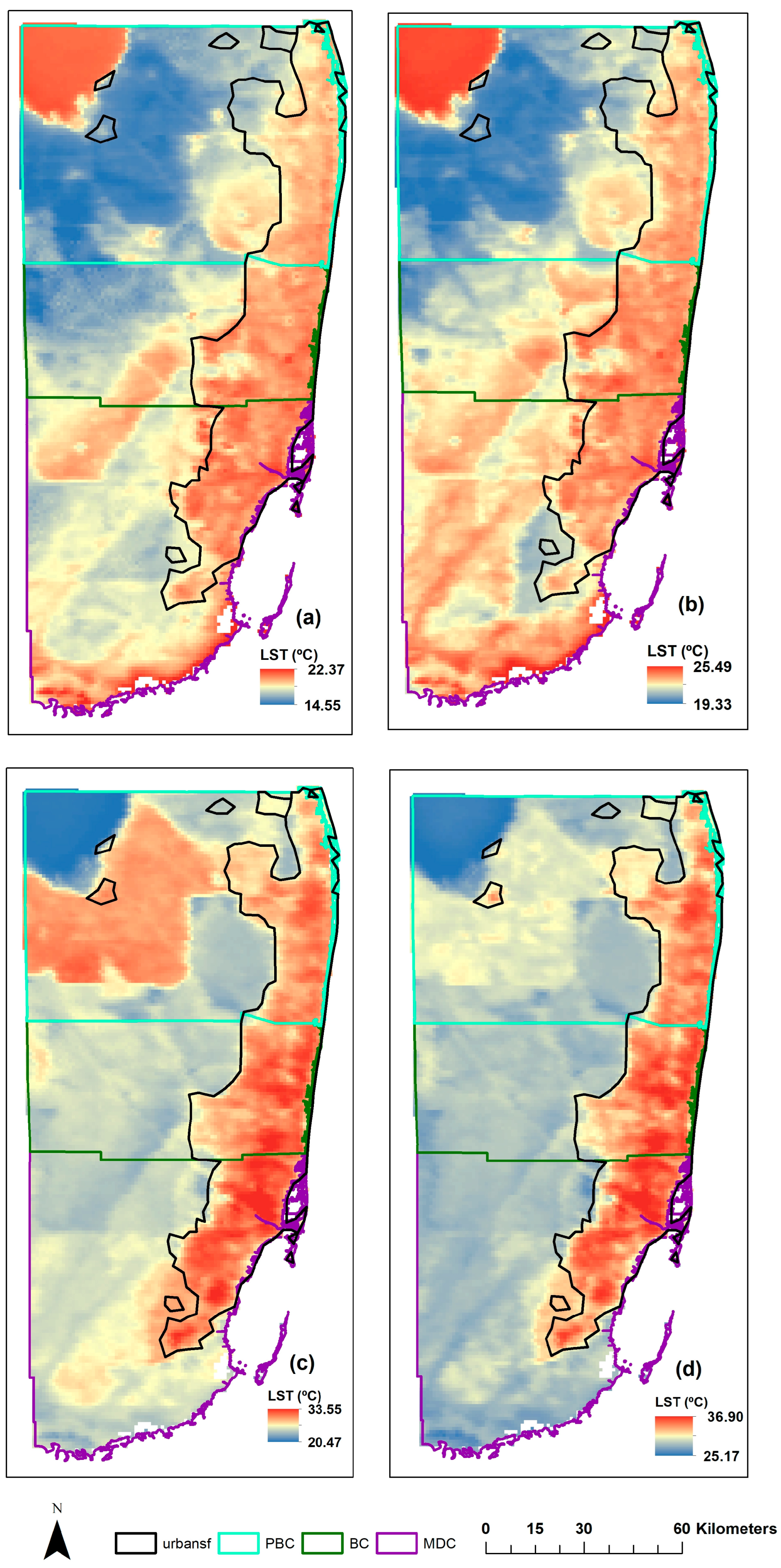
3.1. Spatiotemporal Distributions of LST

Observations in this analysis can be divided into four distinct categories: (a) Dry Night; (b) Wet Night; (c) Dry Day; and (d) Wet Day. The LST has higher values on the eastern side of the study area, which includes urban and coastal areas. The LST is higher during the wet season, ranging from a high of 36.90 °C to a low of 19.33 °C. The dry season has lower LST values, ranging from a high of 33.55 °C to a low of 14.55 °C. During the night, LST has lower values than during the daytime. The nighttime spatial distribution shows that the higher LST values during the night are located throughout the study area, while higher LST values during the daytime are mostly in coastal areas. In fact, the night LST is higher near Lake Okeechobee and around the coastline in the southern part of the study area which is shown to be cooler during the day. Figure 3 shows the LST in °C for the four models: Dry Night, Wet Night, Dry Day, and Wet Day.
LST is highest during the Wet Day period with a mean value of 30.34 °C. The Dry Night period has the lowest LST with the mean temperature of 17.90 °C. The ranking of LST values from Wet Day, Dry Day, to Wet Night to Dry Night is also consistent at the county level for the three counties studied. The LST is highest for MDC which is also the county furthest to the south. The range and mean LST by county, study area, season, and time of day are provided in the Supplementary Materials (Table S1). The standard deviation of the Day results shows a spread-out range of LST values with an MSA value of 2.70 for Dry Day while the standard deviation for the Night shows that the values are closer and do not have a wide range of LST values with a lower MSA standard deviation value of 1.05.

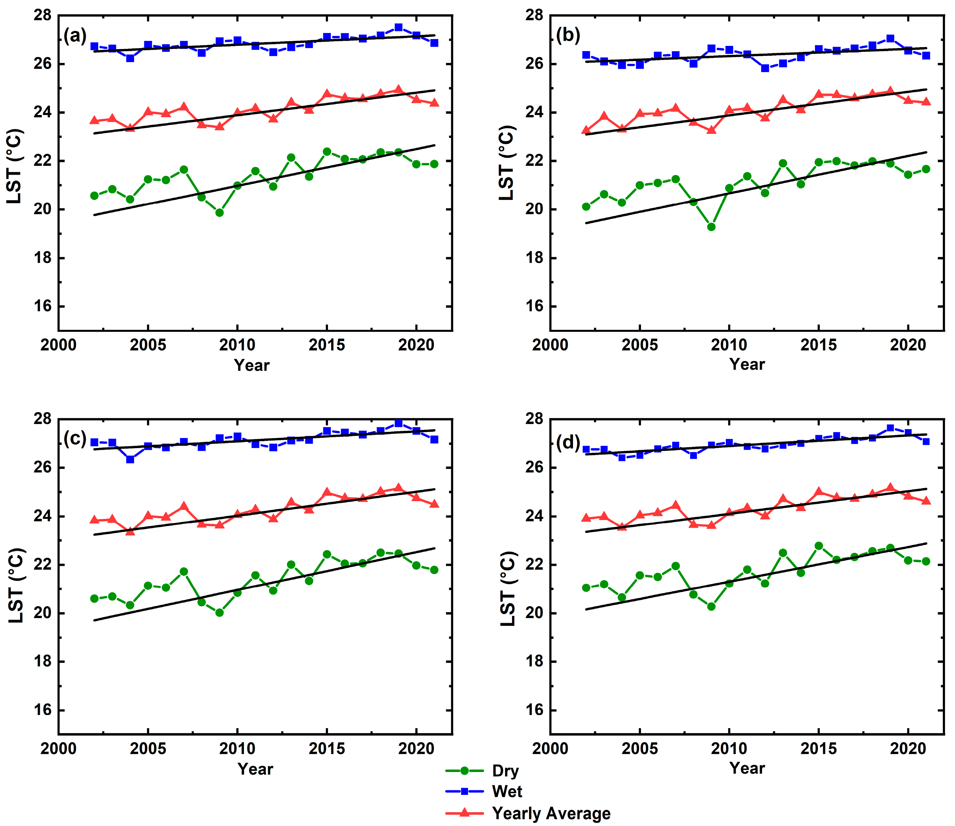
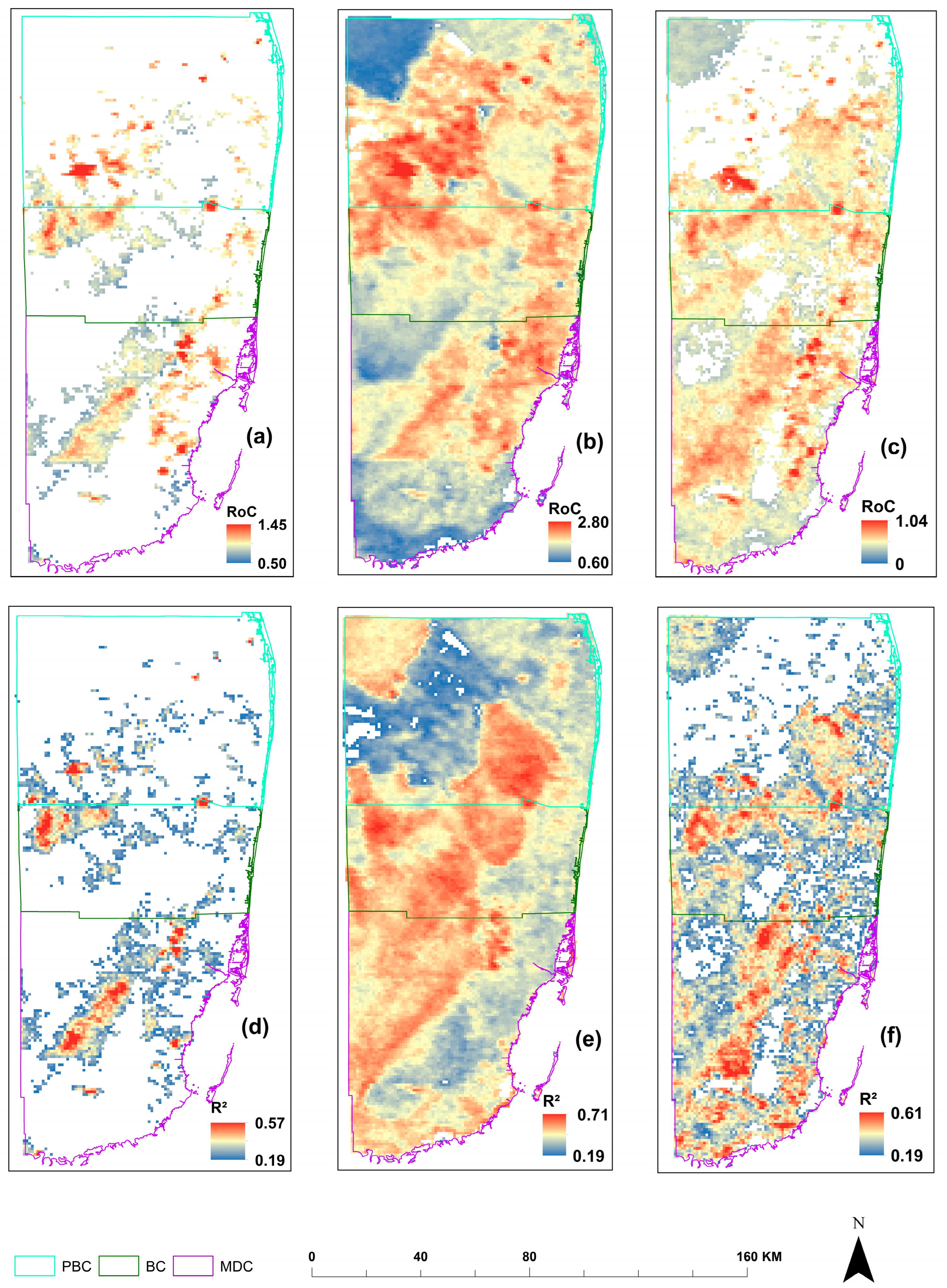
3.2. LST Trend Analysis

LST is consistently elevated during the wet season compared to the dry season each year between 2002 and 2021, inclusive, as Figure 4 shows. An elevated LST during the wet season remains unchanged in the study area, and specifically throughout each of the counties studied. In addition, during the years evaluated, LST continually increased each year throughout the study area, which may be due to increased urbanization.
The three counties and the MSA show similar trends. There is a large drop between the years 2006 (21 °C) and 2009 (19 °C) [44,45].
Table 2 shows the linear regression statistics for the trend analysis. Most of the R2 for each of the regression models are around 0.50, accounting for about half of the change in LST. The RoC of each of the regressions ranged from 0.290 °C/decade to 1.560 °C/decade. The wet season regressions show a relatively low RoC compared to the dry season regressions. BC Dry has the highest RoC with 1.560 °C/decade. The lowest RoC was shown for PBC Wet at 0.290 °C/decade.
Figure 5 displays the spatial distribution of the pixel-level LST trend in the MSA. Only pixels with a p-value less than 0.05 are shown. A larger number of counties show a significant RoC in the dry season relative to the wet season and yearly average (Figure 5). The only pixels that are not significant in the dry season are located around Lake Okeechobee. The dry season has the highest RoC, 2.80 (°C/decade) in the western part of PBC south of Lake Okeechobee. There are a few hot spots of RoC in BC with the highest RoC being 2.13 °C/decade in the northern part. There are a few hot spot locations in MDC in the eastern part of the county with the highest being 2.12 °C/decade. The wet season was lower than the dry season with the highest RoC being 1.04 °C/decade. The highest RoC of the MSA is in the eastern part of MDC. The hotspots for RoC in BC are in the northern part of the county as well as a few hot spot areas in the southeastern part of the county. The highest RoC in BC is in the northern part of the county at the borderline of PBC with 0.99 °C/decade. The rural RoC hotspots are in the western part of the county with a value of 0.90 °C/decade. The yearly average has the least number of significant values with a RoC of 1.45 °C/decade with the highest value of the yearly average being in the eastern part of MDC. With significant pixels being shown for yearly average, the hot spots of the RoC are shown within the western part of PBC with a RoC of 1.35 °C/decade. The northern part of BC has the highest values in the county being 1.38 °C/decade. These pixel trend results show that there is a high LST trend in rural areas compared to urban areas. The rural areas are located in the western part of the MSA where the wetlands are located. The urban areas are located along the coast of the MSA. The trend seems to be telling of the urban growth going towards the rural wetland areas. The results for the R2 for the dry season show that the higher model accuracy of around 60% is in the western part of the study area which is more rural. The lower accuracy of the dry season is in the urban areas. The wet season is showing more of a mix between the average being all over the study area.

3.3. LST Explanatory Factors

Twelve of the 16 multivariate regression models tested have R2 values greater than 60%, indicating that the models explain much of the variation in LST, the dependent variable, as Table 3 shows. As expected, the Tree Canopy variable in Dry Day has high negative values for the MSA (−12.924), PBC (−20.875), and MDC (−6.168). The NDVI variable on the other hand has a positive coefficient with a value of 12.274 in PBC and 7.028 in the MSA. As expected, Impervious Surfaces are positively correlated to LST in all three counties as well as for the MSA. Precipitation has a powerful positive correlation for Dry Day BC (7.709). The MSA as well as PBC and MDC have a smaller positive correlation for precipitation which suggests there may be less precipitation in BC compared to the other counties. Distance to the Roads has a strong negative coefficient for Dry Day MDC (−10.443). This is surprising and is different from the other counties and the MSA which have lower coefficients.
Dry Night results are different from Dry Day. The NDVI variable for Dry Night is the opposite from Dry Day with high negative coefficients for the MSA (−6.864) and PBC (−8.991). Precipitation has positive correlations for the MSA (3.317), PBC (3.485), and BC (5.702).
Wet Day has similar results to the analysis from Dry Day. Tree Canopy Wet Day has strong negative correlations with LST for the MSA (−6.110), PBC (−10.934), and MDC (−11.276). Distance to Roads has a strong negative correlation with MDC (−9.510) compared to the other counties and the MSA. Like Dry Day, Precipitation has a strong positive correlation for BC (9.353). Wet Night has strong negative correlations on NDVI for the MSA (−6.919), PBC (−6.723), and BC (−6.052).
Tree Canopy and NDVI had significant effects on LST, but it was inconsistent between the daytime and nighttime analysis. For example, there were positive correlations for NDVI during the daytime but were negative during the nighttime with the opposite effect for Tree Canopy with negative correlation during the daytime but positive during the nighttime. Among the significant factors, Tree Canopy is shown as the factor that results in the cooling of LST while Impervious Surfaces show the opposite causing LST to increase. The issue of LST measurement accuracy and validation is an issue that has been identified in the literature. The problem is magnified in areas with significant vegetation or tree canopy with ground measurements used to conduct validation studies [46].

4. Discussion

Research about LST spatiotemporal patterns and trends is needed to inform mitigation planning and decisions. Bera et al. [8] investigated trends in India during the winter and summer. The current study examines dry and wet seasons and pixel trends. With a three-level multiscale analysis used for both the explanatory factors and trend analyses, it helped provide a broader perspective of the spatial relationships. The graphs in Figure 4 show that MDC and BC have higher LST values than PBC. This gives responders information on what counties to investigate further for decisions on adding greenery and where mitigation efforts are most beneficial. The multiscale view of pixels in Figure 5 provides a localized perspective for assessing trends and determining critical areas for future evaluation. Figure 5 suggests an LST trend of increasing the LST values in rural areas which would not have been determined from using data at just one scale. This could be a result of urbanization in South Florida. A shift is occurring from coastal housing areas in the eastern part of the MSA to inland areas with new development in the western part of the study area and the inland rural areas [47]. The urban area of the MSA expanded about 1.37 times from 1992 to 2016 with PBC expanding faster than BC and MDC [6]. The yearly average has less significant values compared to the dry or wet seasons. The RoC is higher during the dry season compared to the wet season.
The trend analysis suggests that LST is rising over time within the MSA. LST’s RoC is more pronounced during the dry season than the wet season, as Figure 4 shows. Trend change rates were investigated annually for a 20-year span at global and pixel scales in previous studies such as Wang et al. [14]. The current study adds the investigation of LST at the MSA, county, and pixel levels. The fall in LST during 2020 during both seasons may have been caused by the societal shutdown during the COVID-19 pandemic resulting in less people travelling to and working in the city during the day.
The LST is a variable that is related to other geographical, climatological, and hydrological elements [28]. As expected, the explanatory variables related to pavement and buildings have positive coefficients while the land cover Tree Canopy variables have negative coefficients in regression models predicting LST. We examined the relationship between LST and explanatory variable in the MSA and investigated the LST in different views by day and night as well as for the dry or wet seasons. This study has results like Alhawiti et al. [7], as Figure 3 and Table 3 show. Warmer LST values are located within areas with the most pavement and dense buildings.
Proximity to the coast and tree canopy or vegetation have a negative correlation with LST during the day, but this relationship is positive during the night. This result is similar to previous studies for SUHI [12,48,49]. Higher day LST values appear to be contained in coastal urban areas while night values are more spread out in the MSA, as Figure 3 shows. Higher nighttime LST seems to expand to rural areas. During the nighttime, the tree canopy has a positive coefficient, as Table 3 shows, suggesting that a higher tree canopy percentage results in higher LST values. In areas with dense tree coverage, heat is trapped under the tree canopy due to restricted radiative cooling and impaired ventilation [34]. The tree canopy increases the shade effect which reduces the incidences of radiation and cools the LST down [8]. It is important to examine the day and night LST differences in urban heat research. In previous studies, as well as the current one, there are differences between explanatory factors and the impacts with the LST values during day and night.
Results in BC have night and day coefficients for the tree canopy with opposite signs. Additional research is needed to explain these results and to understand how BC is different from the other counties studied. A possible hypothesis is that since the county is between PBC and MDC it does not have as much greenery and tree canopy, resulting in a more urbanized location with Fort Lauderdale having a large impact. PBC has Lake Okeechobee and surroundings of the upper wetlands and MDC has the western part of the county being in the Everglades with extensive greenery. Lake Okeechobee is another area that has large differences in night and day spatial distribution of LST. Like the tree canopy, water seems to be warmer at night than during the day. As expected, Table 3 shows that Impervious Surfaces have positive coefficients for all distributions, suggesting that greater impervious services result in increased LST. Almost all the linear regression models have R2 values greater than 50%. The R2 value for MDC’s Wet Night model is only 26% compared with 37% for Dry Night. The rest of the R2 values for MDC are above 60%. The lower values may occur because LST can change along the coast and water at night with water being known to be warmer at night.

5. Conclusions

The relationship between LST trends and explanatory variables in South Florida is examined in this study using a three-level multiscale analysis. The annual and seasonal day–night trends of LST and the relationship of explanatory variables on LST are explored using MODIS imagery data from GEE for the years 2002 to 2021 in the MSA. The results indicate that LST values are rising with a positive trend throughout the 20-year study period with RoC values ranging from 0.29 °C/decade to 1.56 °C/decade. Results over the study period indicate that the wet season has a smaller RoC compared to the dry season. The pixel spatial distributions show that the RoC for the 20-year period is primarily in rural areas and less apparent in urban areas. New development in rural areas may affect the RoC. The relationship between LST and physical and climatic explanatory variables suggests that Impervious Surfaces have the greatest impact on LST. This is consistent with the results from previous studies in other locations. The results from this study, however, indicate that during the night, the Tree Canopy variable has a positive coefficient which suggests that the Tree Canopy causes the LST to increase, while during the day, the Tree Canopy has a negative coefficient. The Distance to the Coast variable changes from day to night as well. Nighttime spatial distributions show a change in LST along the southern part of the MSA, along the southern coastline. In the daytime spatial distributions, the warmer LST values are more common in urban areas where the ocean and water are cooler.
These results can help practitioners, including urban planners, emergency responders, and other decision makers, understand the spatial distribution of LST as well as the causes of higher LST values. Further research is needed to investigate predicted LST values correlated to trends of current and past LST values in the MSA and to link this information with data on heat-related illnesses to determine if there are significant changes in heat-related illnesses between urban and rural areas.

Supplementary Materials

The following supporting information can be downloaded at: https://www.mdpi.com/article/10.3390/geomatics4010001/s1, Table S1: LST distribution statistics.

Author Contributions

Conceptualization, W.L.; methodology, W.L. and A.D.S.; formal analysis, A.D.S. and W.L.; data curation, A.D.S.; writing—original draft, A.D.S.; writing—review and editing, W.L; supervision, W.L. All authors have read and agreed to the published version of the manuscript.

Funding

This research is supported by Florida Atlantic University College of Science Research Fellowship.

Data Availability Statement

No new data were created or analyzed in this study. Data sharing is not applicable to this article.

Acknowledgments

We would like to thank the three anonymous reviewers and editors for providing valuable comments and suggestions which helped improve the manuscript greatly.

Conflicts of Interest

The authors declare no conflicts of interest. The funders had no role in the design of the study; in the collection, analyses, or interpretation of data; in the writing of the manuscript, or in the decision to publish the results.

References

  1. Hibbard, K.; Hoffman, F.; Huntzinger, D.N.; West, T. Changes in Land Cover and Terrestrial Biogeochemistry. 2017. Available online: http://digitalcommons.unl.edu/usdeptcommercepubhttp://digitalcommons.unl.edu/usdeptcommercepub/583 (accessed on 3 May 2023).
  2. Dissanayake, D.; Morimoto, T.; Murayama, Y.; Ranagalage, M.; Handayani, H.H. Impact of urban surface characteristics and socio-economic variables on the spatial variation of land surface temperature in Lagos City, Nigeria. Sustainability 2019, 11, 25. [Google Scholar] [CrossRef]
  3. Harmay, N.S.M.; Choi, M. The urban heat island and thermal heat stress correlate with climate dynamics and energy budget variations in multiple urban environments. Sustain. Cities Soc. 2023, 91. [Google Scholar] [CrossRef]
  4. Huang, G.; Zhou, W.; Cadenasso, M. Is everyone hot in the city? Spatial pattern of land surface temperatures, land cover and neighborhood socioeconomic characteristics in Baltimore, MD. J. Environ. Manag. 2011, 92, 1753–1759. [Google Scholar] [CrossRef] [PubMed]
  5. Gusso, A.; Bordin, F.; Veronez, M.; Cafruni, C.; Lenz, L.; Crija, S. Multitemporal Analysis of Thermal Distribution Characteristics for Urban Heat Islands Management. 1985. Available online: http://www.sciforum.net/conference/wsf-4 (accessed on 13 March 2023).
  6. Al Rifat, S.A.; Liu, W. Quantifying spatiotemporal patterns and major explanatory factors of urban expansion in miami metropolitan area during 1992–2016. Remote Sens. 2019, 11, 2493. [Google Scholar] [CrossRef]
  7. Alhawiti, R.H.; Mitsova, D. Using Landsat-8 Data to Explore the Correlation Between Urban Heat Island and Urban Land Uses. 2016. Available online: http://www.ijret.org (accessed on 11 March 2023).
  8. Bera, D.; Das Chatterjee, N.; Ghosh, S.; Dinda, S.; Bera, S. Recent trends of land surface temperature in relation to the influencing factors using Google Earth Engine platform and time series products in megacities of India. J. Clean. Prod. 2022, 379, 134735. [Google Scholar] [CrossRef]
  9. Halder, B.; Bandyopadhyay, J.; Banik, P. Monitoring the effect of urban development on urban heat island based on remote sensing and geo-spatial approach in Kolkata and adjacent areas, India. Sustain. Cities Soc. 2021, 74, 103186. [Google Scholar] [CrossRef]
  10. Hou, H.; Su, H.; Liu, K.; Li, X.; Chen, S.; Wang, W.; Lin, J. Driving forces of UHI changes in China’s major cities from the perspective of land surface energy balance. Sci. Total. Environ. 2022, 829, 154710. [Google Scholar] [CrossRef]
  11. Xi, M.; Zhang, W.; Li, W.; Liu, H.; Zheng, H. Distinguishing Dominant Drivers on LST Dynamics in the Qinling-Daba Mountains in Central China from 2000 to 2020. Remote. Sens. 2023, 15, 878. [Google Scholar] [CrossRef]
  12. You, M.; Lai, R.; Lin, J.; Zhu, Z. Quantitative analysis of a spatial distribution and driving factors of the urban heat island effect: A case study of Fuzhou Central Area, China. Int. J. Environ. Res. Public Health 2021, 18, 13088. [Google Scholar] [CrossRef]
  13. Liu, W.; Feddema, J.; Hu, L.; Zung, A.; Brunsell, N. Seasonal and diurnal characteristics of land surface temperature and major explanatory factors in Harris County, Texas. Sustainability 2017, 9, 2324. [Google Scholar] [CrossRef]
  14. Wang, Y.R.; Hessen, D.O.; Samset, B.H.; Stordal, F. Evaluating global and regional land warming trends in the past decades with both MODIS and ERA5-Land land surface temperature data. Remote. Sens. Environ. 2022, 280, 113181. [Google Scholar] [CrossRef]
  15. Verbesselt, J.; Hyndman, R.; Newnham, G.; Culvenor, D. Detecting trend and seasonal changes in satellite image time series. Remote Sens. Environ. 2010, 114, 106–115. [Google Scholar] [CrossRef]
  16. Pandey, P.C.; Chauhan, A.; Maurya, N.K. Evaluation of earth observation datasets for LST trends over India and its implication in global warming. Ecol. Inform. 2022, 72, 101843. [Google Scholar] [CrossRef]
  17. Sun, D.; Kafatos, M. Note on the NDVI-LST relationship and the use of temperature-related drought indices over North America. Geophys. Res. Lett. 2007, 34. [Google Scholar] [CrossRef]
  18. Chen, L.; Li, M.; Huang, F.; Xu, S. Relationships of LST to NDBI and NDVI in Wuhan City based on Landsat ETM+ image. In Proceedings of the 6th International Congress on Image and Signal Processing (CISP), Hangzhou, China, 16–18 December 2013; pp. 840–845. [Google Scholar] [CrossRef]
  19. Wang, X.; Zhang, Y.; Yu, D. Exploring the Relationships between Land Surface Temperature and Its Influencing Factors Using Multisource Spatial Big Data: A Case Study in Beijing, China. Remote. Sens. 2023, 15, 1783. [Google Scholar] [CrossRef]
  20. Xiao, R.-b.; Ouyang, Z.-y.; Zheng, H.; Li, W.-f.; Schienke, E.W.; Wang, X.-K. Spatial pattern of impervious surfaces and their impacts on land surface temperature in Beijing, China. J. Environ. Sci. 2007, 19, 250–256. [Google Scholar] [CrossRef] [PubMed]
  21. Jumai, M.; Kasimu, A.; Liang, H.; Tang, L.; Aizizi, Y.; Zhang, X. A Study on the Spatial and Temporal Variation of Summer Surface Temperature in the Bosten Lake Basin and Its Influencing Factors. Land 2023, 12, 1185. [Google Scholar] [CrossRef]
  22. Kandel, H.; Melesse, A.; Whitman, D. An analysis on the urban heat island effect using radiosonde profiles and Landsat imagery with ground meteorological data in South Florida. Int. J. Remote. Sens. 2016, 37, 2313–2337. [Google Scholar] [CrossRef]
  23. The Urban and Rural Classifications. Available online: https://www.census.gov (accessed on 7 December 2023).
  24. Beginning of the South Florida Dry Season. Miami, FL. 2009. Available online: https://www.weather.gov/media/mfl/news/2009RainySeasonSummary.pdf (accessed on 15 May 2023).
  25. ACS. American Community Survey. Available online: https://www.census.gov/programs-surveys/acs (accessed on 13 February 2021).
  26. Wan, Z.; Li, Z.-L. A Physics-Based Algorithm for Retrieving Land-Surface Emissivity and Temperature from EOS/MODIS Data. IEEE Trans. Geosci. Remote. Sens. 1997, 35, 980–996. [Google Scholar] [CrossRef]
  27. Guillevic, P.C.; Göttsche, F.; Nickeson, J.; Hulley, G.; Ghent, D.; Yu, Y.; Trigo, I.; Hook, S.; Sobrino, J.A.; Remedios, J.; et al. Land Surface Temperature Product Validation Best Practice Protocol, version 1.1; Land Product Validation Subgroup (WGCV/CEOS): Washington, DC, USA, 2018; p. 58. [Google Scholar] [CrossRef]
  28. Duan, S.B.; Huang, C.; Liu, X.; Liu, M.; Sun, Y.; Gao, C. Spatio-Temporal Distribution Characteristics of Global Annual Maximum Land Surface Temperature Derived from MODIS Thermal Infrared Data From 2003 to 2019. IEEE J. Sel. Top. Appl. Earth Obs. Remote Sens. 2022, 15, 4690–4697. [Google Scholar] [CrossRef]
  29. Gorelick, N.; Hancher, M.; Dixon, M.; Ilyushchenko, S.; Thau, D.; Moore, R. Google Earth Engine: Planetary-scale geospatial analysis for everyone. Remote Sens. Environ. 2017, 202, 18–27. [Google Scholar] [CrossRef]
  30. Abunnasr, Y.; Mhawej, M. Towards a combined Landsat-8 and Sentinel-2 for 10-m land surface temperature products: The Google Earth Engine monthly Ten-ST-GEE system. Environ. Model. Softw. 2022, 155. [Google Scholar] [CrossRef]
  31. Feng, Y.; Gao, C.; Tong, X.; Chen, S.; Lei, Z.; Wang, J. Spatial patterns of land surface temperature and their influencing factors: A case study in Suzhou, China. Remote Sens. 2019, 11, 182. [Google Scholar] [CrossRef]
  32. Winbourne, J.B.; Jones, T.S.; Garvey, S.M.; Harrison, J.L.; Wang, L.; Li, D.; Templer, P.H.; Hutyra, L.R. Tree transpiration and urban temperatures: Current understanding, implications, and future research directions. BioScience 2020, 70, 576–588. [Google Scholar] [CrossRef]
  33. Morabito, M.; Crisci, A.; Guerri, G.; Messeri, A.; Congedo, L.; Munafò, M. Surface urban heat islands in Italian metropolitan cities: Tree cover and impervious surface influences. Sci. Total. Environ. 2020, 751, 142334. [Google Scholar] [CrossRef]
  34. Wujeska-Klause, A.; Pfautsch, S. The best urban trees for daytime cooling leave nights slightly warmer. Forests 2020, 11, 945. [Google Scholar] [CrossRef]
  35. Duveiller, G.; Hooker, J.; Cescatti, A. The mark of vegetation change on Earth’s surface energy balance. Nat. Commun. 2018, 9, 679. [Google Scholar] [CrossRef]
  36. Yang, L.; Huang, C.; Wylie Usgs Eros, B.K.; Coan, J.M. An Approach for Mapping Large-Area Impervious Surfaces: Synergistic use of Landsat-7 ETM+ and High Spatial Resolution Imagery. Can. J. Remote Sens. 2003, 29, 230–240. [Google Scholar] [CrossRef]
  37. Hartmann, D.L. Chapter 4 The Energy Balance of the Surface. Int. Geophys. 1994, 56, 81–114. [Google Scholar] [CrossRef]
  38. Si, M.; Li, Z.-L.; Nerry, F.; Tang, B.-H.; Leng, P.; Wu, H.; Zhang, X.; Shang, G. Spatiotemporal pattern and long-term trend of global surface urban heat islands characterized by dynamic urban-extent method and MODIS data. ISPRS J. Photogramm. Remote Sens. 2022, 183, 321–335. [Google Scholar] [CrossRef]
  39. Prasetya, T.A.E.; Devi, R.M.; Fitrahanjani, C.; Wahyuningtyas, T.; Muna, S. Systematic assessment of the warming trend in Madagascar’s mainland daytime land surface temperature from 2000 to 2019. J. Afr. Earth Sci. 2022, 189, 104502. [Google Scholar] [CrossRef]
  40. Quan, J.; Zhan, W.; Chen, Y.; Wang, M.; Wang, J. Time series decomposition of remotely sensed land surface temperature and investigation of trends and seasonal variations in surface urban heat islands. J. Geophys. Res. Atmos. 2016, 121, 2638–2657. [Google Scholar] [CrossRef]
  41. Zhao, B.; Mao, K.; Cai, Y.; Shi, J.; Li, Z.; Qin, Z.; Meng, X.; Shen, X.; Guo, Z. A combined Terra and Aqua MODIS land surface temperature and meteorological station data product for China from 2003 to 2017. Earth Syst. Sci. Data 2020, 12, 2555–2577. [Google Scholar] [CrossRef]
  42. Guo, A.; Yang, J.; Sun, W.; Xiao, X.; Cecilia, J.X.; Jin, C.; Li, X. Impact of urban morphology and landscape characteristics on spatiotemporal heterogeneity of land surface temperature. Sustain. Cities Soc. 2020, 63, 102443. [Google Scholar] [CrossRef]
  43. Jung, C.; Lee, Y.; Cho, Y.; Kim, S. A study of spatial soil moisture estimation using a multiple linear regression model and modis land surface temperature data corrected by conditional merging. Remote Sens. 2017, 9, 870. [Google Scholar] [CrossRef]
  44. Verdi, R.J.; Tomlinson, S.A.; Marella, R.L. Florida. Department of Transportation., Florida. Department of Environmental Protection, and Geological Survey (U.S.). In The Drought of 1998–2002: Impacts on Florida’s Hydrology and Landscape; U.S. Deptartment of the Interior, U.S. Geological Survey: Reston, VA, USA, 2006. [Google Scholar]
  45. National Weather Service. NOWData—NOAA Online Weather Data; National Weather Service: Silver Spring, MD, USA, 2018. [Google Scholar]
  46. Wang, W.; Liang, S.; Meyers, T. Validating MODIS land surface temperature products using long-term nighttime ground measurements. Remote Sens. Environ. 2008, 112, 623–635. [Google Scholar] [CrossRef]
  47. Kambly, S.; Moreland, T.R. Land Cover Trends in the Southern Florida Coastal Plain; U.S. Geological Survey: Reston, VA, USA, 2009. Available online: http://www.usgs.gov/pubprod (accessed on 20 June 2023).
  48. Jacobs, C.; Klok, L.; Bruse, M.; Cortesão, J.; Lenzholzer, S.; Kluck, J. Are urban water bodies really cooling? Urban Clim. 2020, 32, 100607. [Google Scholar] [CrossRef]
  49. Chen, H.; Deng, Q.; Zhou, Z.; Ren, Z.; Shan, X. Influence of land cover change on spatio-temporal distribution of urban heat island—A case in Wuhan main urban area. Sustain. Cities Soc. 2022, 79, 103715. [Google Scholar] [CrossRef]
Figure 2. Methodology flowchart in this study.
Geomatics 04 00001 g002
Figure 3. The spatial distributions of daytime and nighttime LST shown in °C during the dry and wet seasons with the urban areas overlayed (a) Dry Night, (b) Wet Night, (c) Dry Day, and (d) Wet Day.
Geomatics 04 00001 g003
Figure 4. Annual LST trend analysis: (a) MSA, (b) PBC, (c) BC, and (d) MDC.
Geomatics 04 00001 g004
Figure 5. Pixel-level LST trend spatial distribution showing significant pixels of p-value below 0.05 (a) yearly average of RoC, (b) dry season average of RoC, (c) wet season average of RoC, (d) yearly average of R2, (e) dry season average of R2, and (f) wet season average of R2. RoC is shown in °C/decade.
Geomatics 04 00001 g005
Table 1. Explanatory variables and sources used in this study.
VariableDescriptionSourceSpatial Resolution
Tree CanopyTree Canopy Percentage (%)United States Department of Agriculture Forest Service (USDA)
https://data.fs.usda.gov/geodata/rastergateway/treecanopycover
2016 CONUS dataset (assessed on 1 July 2022)
1 Km
Impervious SurfacesImpervious Surfaces Percentage (%)Multi-Resolution Land Characteristics Consortium
Urban Imperviousness 2019 dataset for National Land Cover Dataset (NLCD) Imperviousness; https://www.mrlc.gov/ (assessed on 1 July 2022)
1 Km
NDVINormalized Difference Vegetation Index Multi-Resolution Land Characteristics Consortium
NLCD 2019 data
https://www.mrlc.gov/ (assessed on 1 July 2022)
1 Km
Distance to the CoastDistance to Coastal and Waterway (km)Distance was calculated using the Euclidean distance tool in ArcGIS.
The Florida waterways dataset was retrieved from the Florida Fish and Wildlife Conservation Commission. The coast data were from the US Tiger Census from 2020.
1 Km
Distance to the Roads Distance to Primary Roads
(km)
US Census
https://www.census.gov/geographies/mapping-files/time-series/geo/tiger-line-file.html (assessed on 1 July 2022)
2020 Roads Shapefile
https://www.census.gov/geographies/mapping-files/time-series/geo/tiger-line-file.html (assessed on 10 July 2022)
Distance was calculated using the Euclidean distance tool in ArcGIS.
1 Km
PrecipitationPrecipitation (cm)National Oceanic and Atmospheric Administration (NOAA)
National Weather Service, 5 years average of precipitation.
1 Km
Table 2. Annual LST trend linear regression analysis in MSA, PBC, BC, and MDC.
ModelR2RoC (°C/Decade)p-Value (×10−4)
MSA Wet0.4800.3407.00
MSA Dry0.4511.51011.9
MSA Avg0.5490.9281.85
PBC Wet0.3020.290121
PBC Dry0.3931.53030.9
PBC Avg0.5180.9723.45
BC Wet0.5210.4103.29
BC Dry0.4941.5605.52
BC Avg0.6030.9850.57
MDC Wet0.6610.4300.13
MDC Dry0.4641.4209.40
MDC Avg0.5930.9300.72
Table 3. Sixteen linear regression models for MSA, PBC, BC, and MDC. An asterisk (*) denotes a significance level of <0.05 (two-tailed), while all others have a significance level of <0.001 (two-tailed).
ModelNDVITree
Canopy
Impervious
Surfaces
Distance to RoadsPrecipitationDistance to WaterR2
Dry Day
MSA
7.028−12.9243.648−4.0130.5234.1470.611
Dry Day
PBC
12.274−20.8754.1530.000089*1.2700.0000800.510
Dry Day
BC
−0.385 *3.7392.697−3.0507.7092.3530.764
Dry Day
MDC
−0.50 *−6.1683.344−10.4430.000 *2.5590.647
Dry Night
MSA
−6.8643.6900.107*1.2283.317−2.9460.660
Dry Night
PBC
−8.9912.359−0.037 *−0.000042 *3.4850.0000310.742
Dry Night
BC
−2.651−1.880−0.20*−0.8445.7020.414 *0.686
Dry Night
MDC
−3.1414.5790.4460.268 *−0.000021 *−3.0290.372
Wet Day
MSA
3.969−6.1103.655−3.1882.2841.1510.722
Wet Day
PBC
5.890−10.9343.5470.000 *4.5360.0000510.694
Wet Day
BC
3.3600.140 *2.764−2.6879.3530.491 *0.809
Wet Day
MDC
1.310 *−11.2763.702−9.5100.000*1.5960.635
Wet Night
MSA
−6.9191.643−0.2841.5803.483−2.2460.721
Wet Night
PBC
−6.723−1.2040.070*−0.000041 *2.3820.0000320.850
Wet Night
BC
−6.052−1.291−0.138−0.9963.3761.2770.738
Wet Night
MDC
−2.0811.8080.4830.193 *−0.0000032 *−1.8700.263
Disclaimer/Publisher’s Note: The statements, opinions and data contained in all publications are solely those of the individual author(s) and contributor(s) and not of MDPI and/or the editor(s). MDPI and/or the editor(s) disclaim responsibility for any injury to people or property resulting from any ideas, methods, instructions or products referred to in the content.

