
Use of Smartphone Lidar Technology for Low-Cost 3D Building Documentation with iPhone 13 Pro: A Comparative Analysis of Mobile Scanning Applications

Abstract
:1. Introduction
2. Related Works
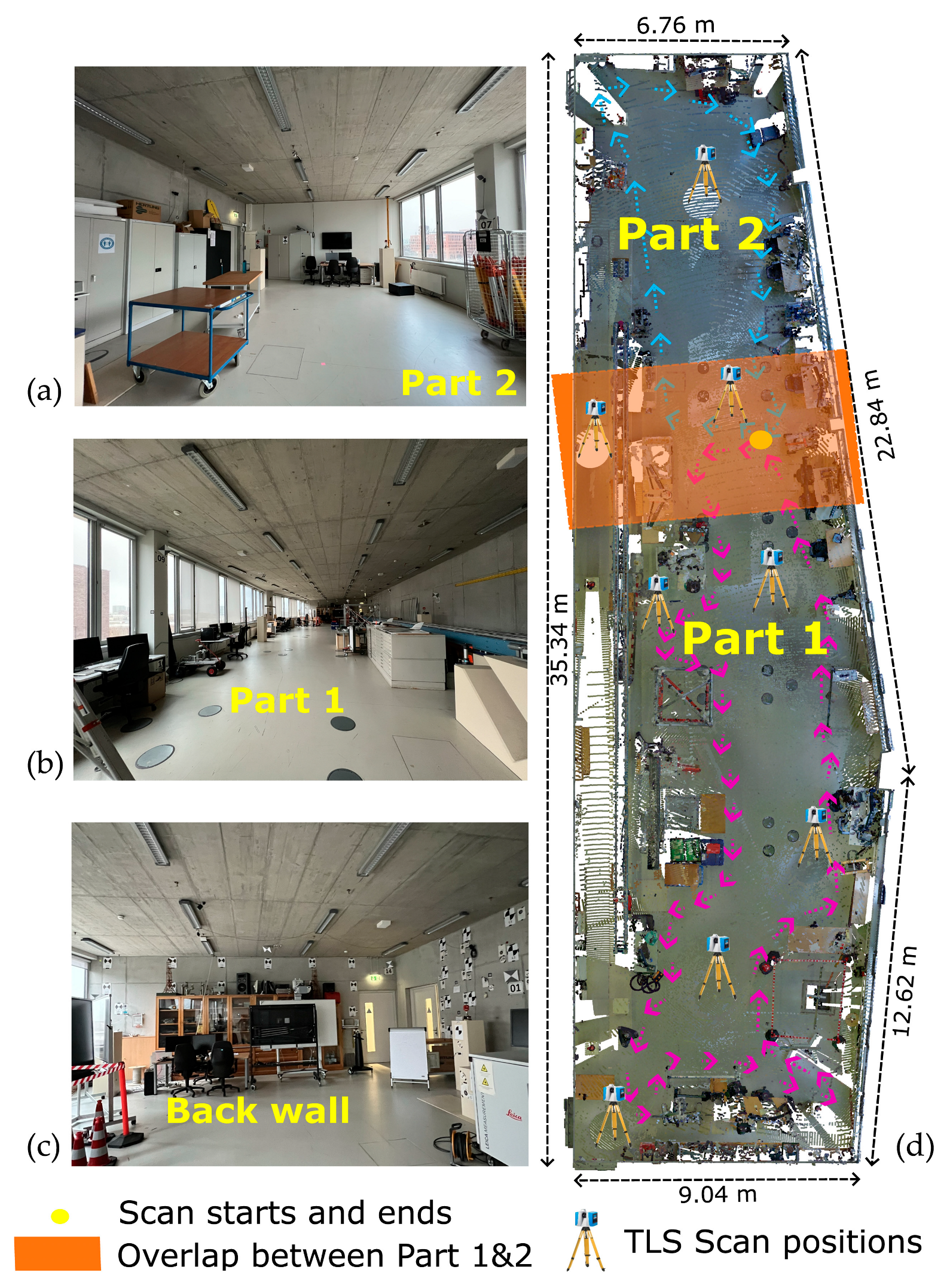
3. Materials and Methods
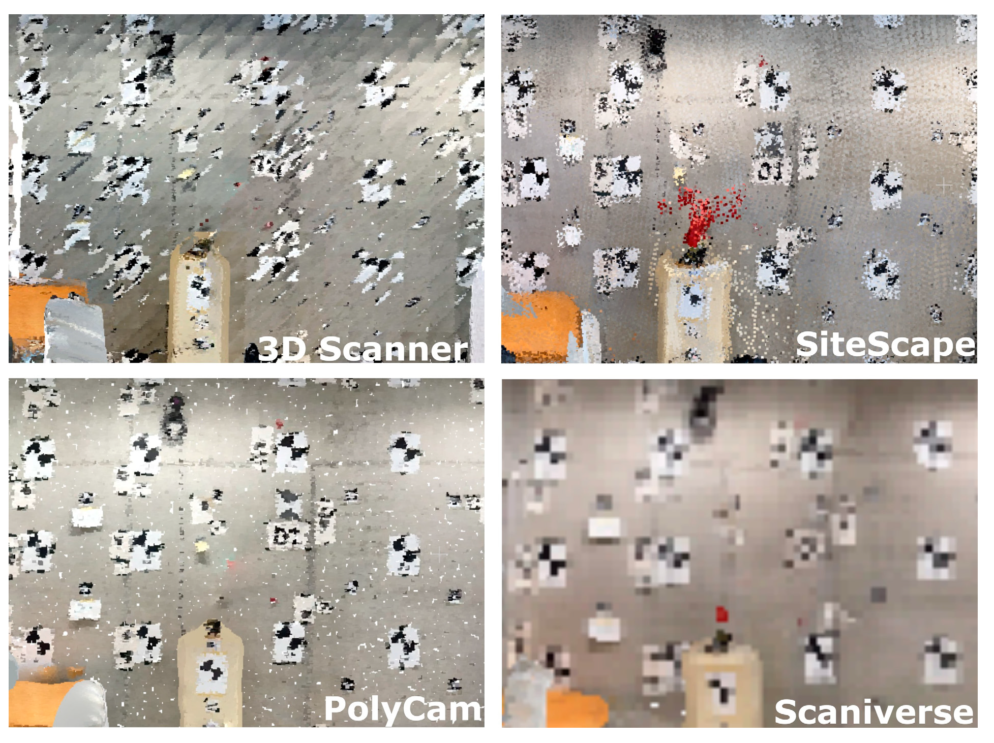
3.1. 3D Scanner App
3.2. PolyCam
3.3. SiteScape
3.4. Scaniverse
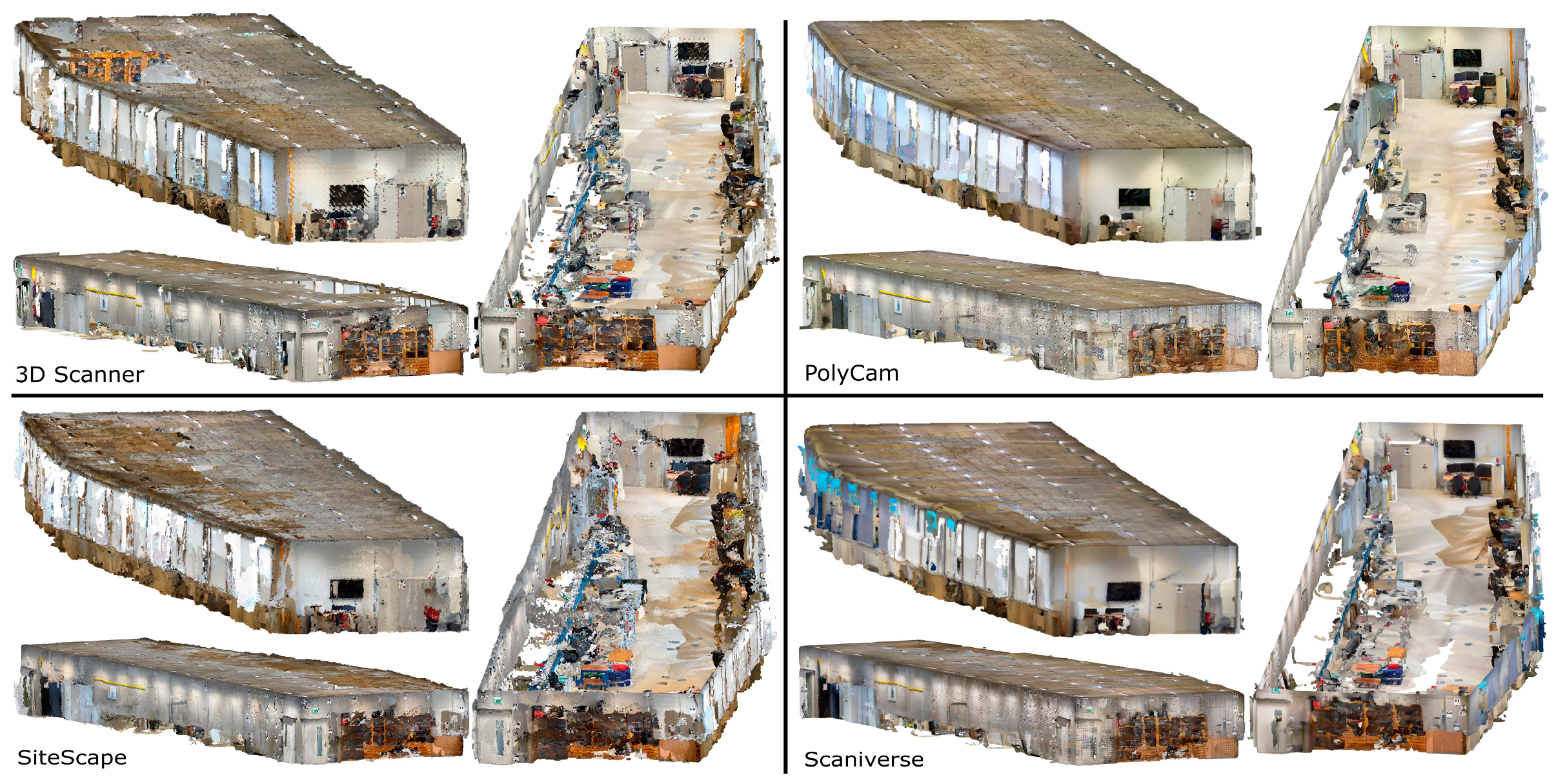
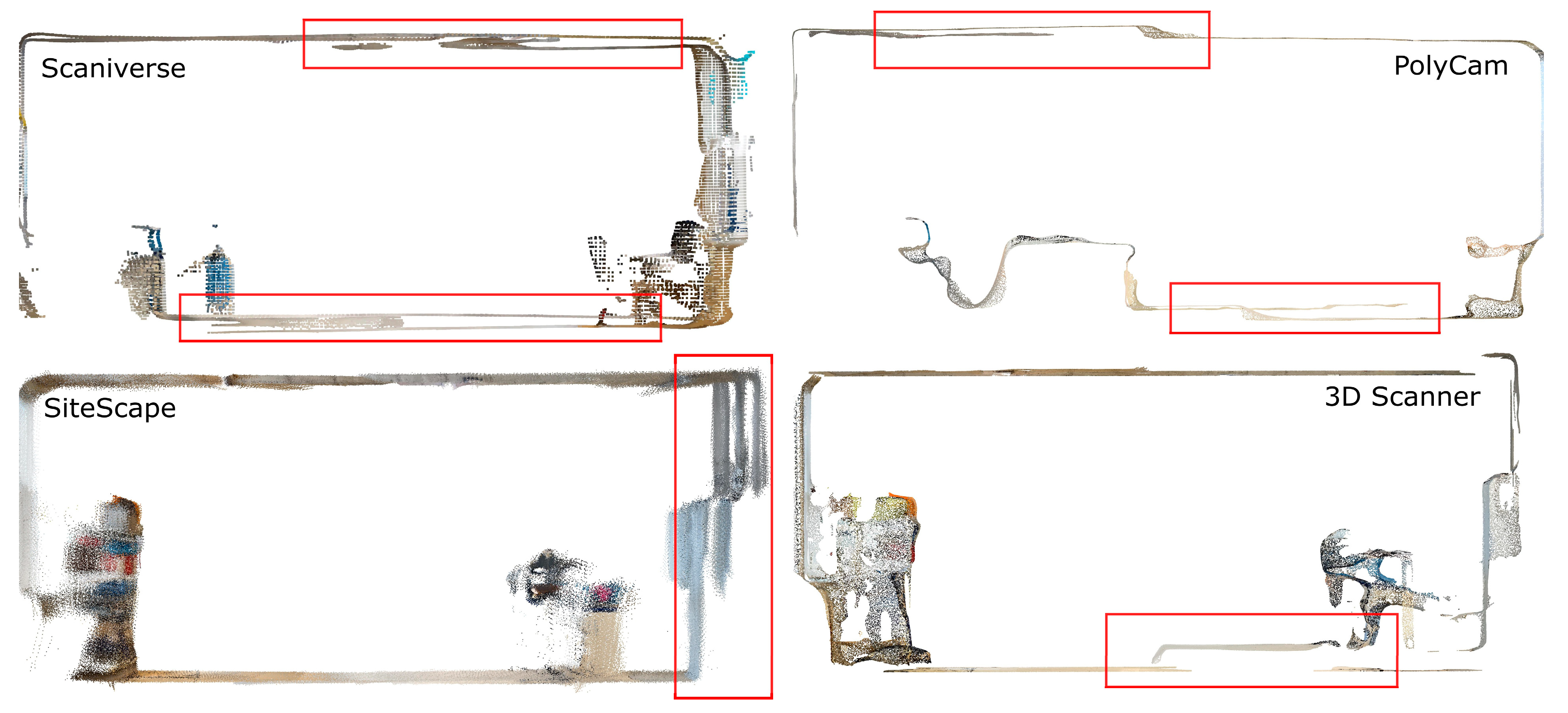
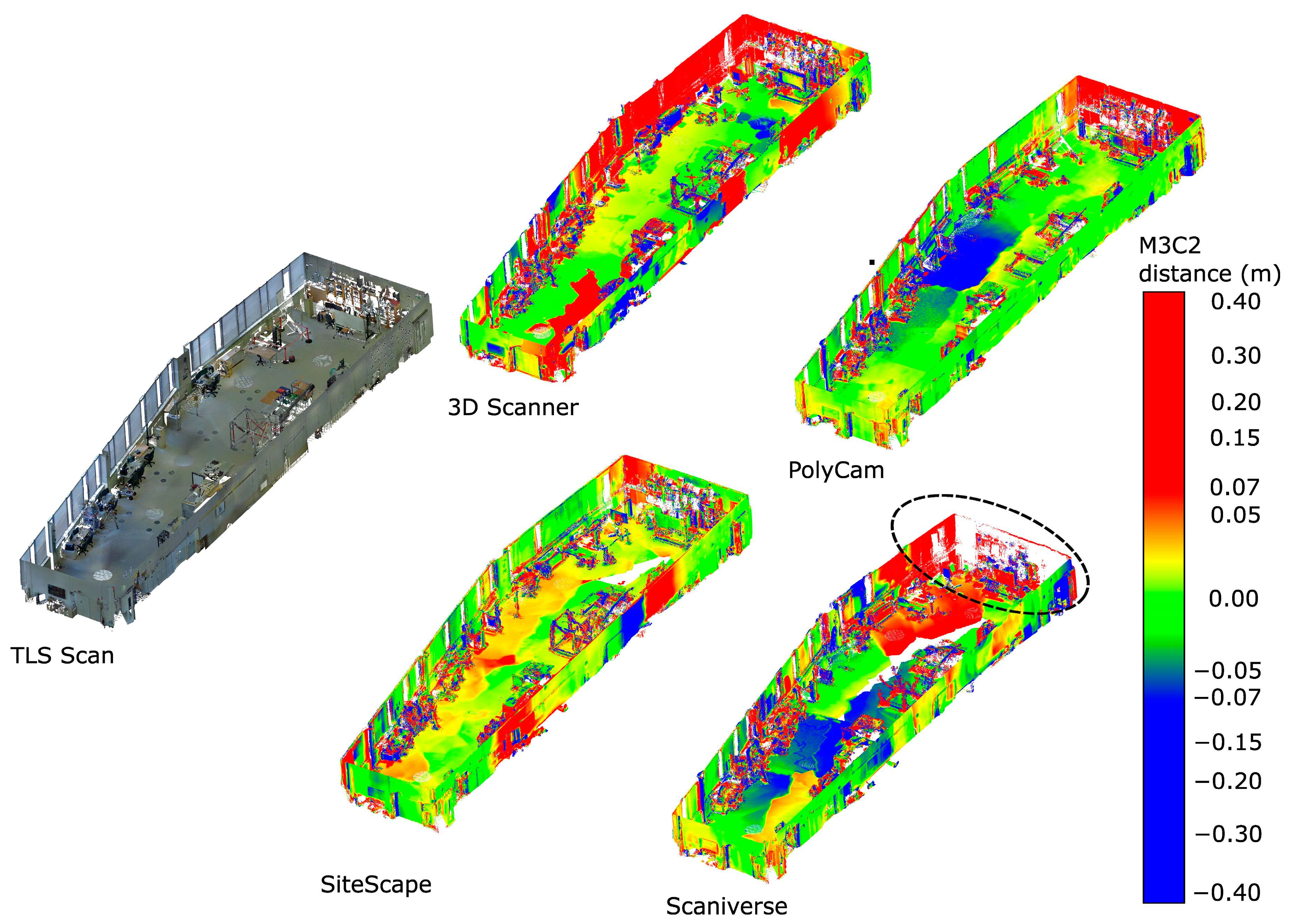
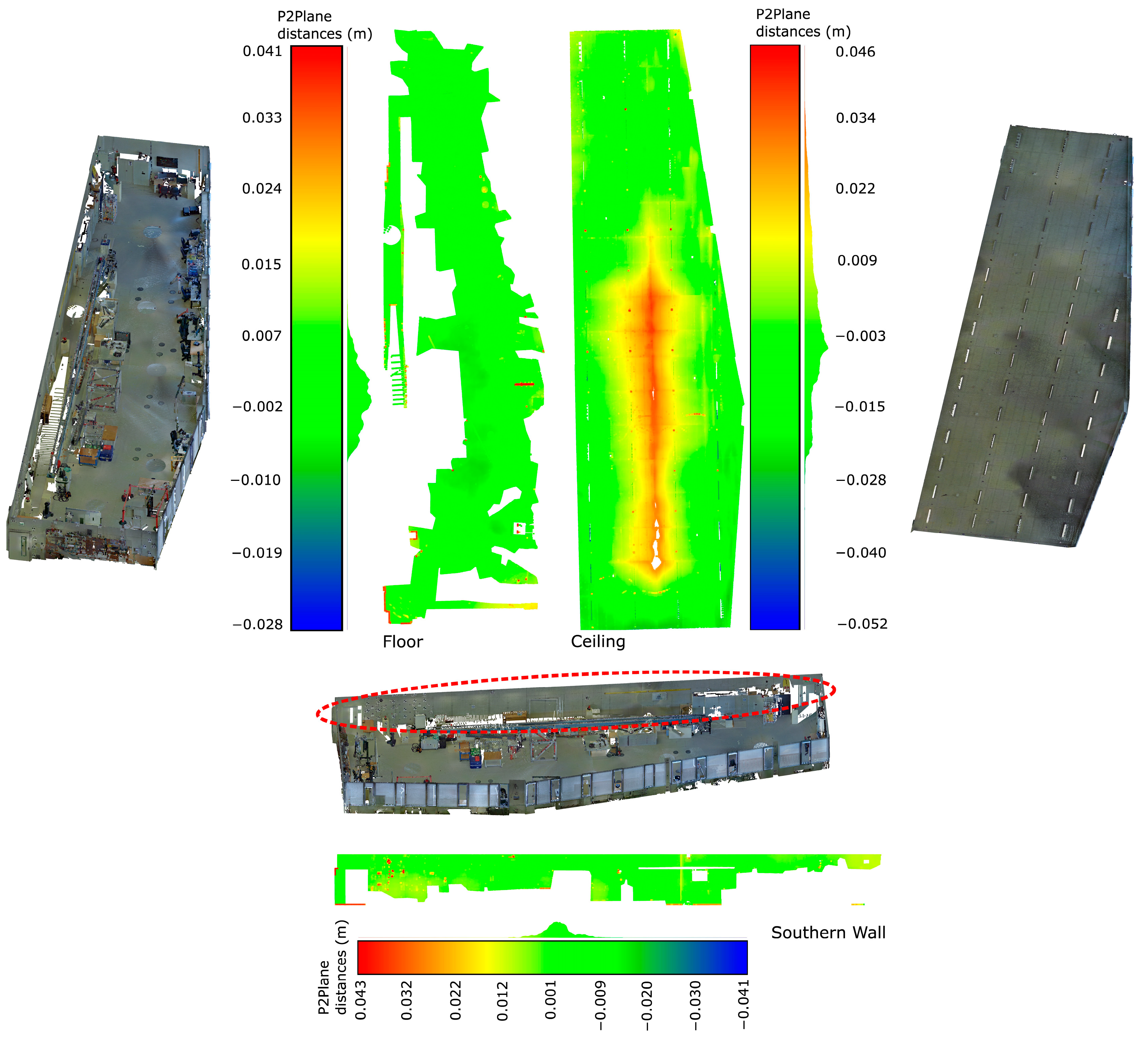
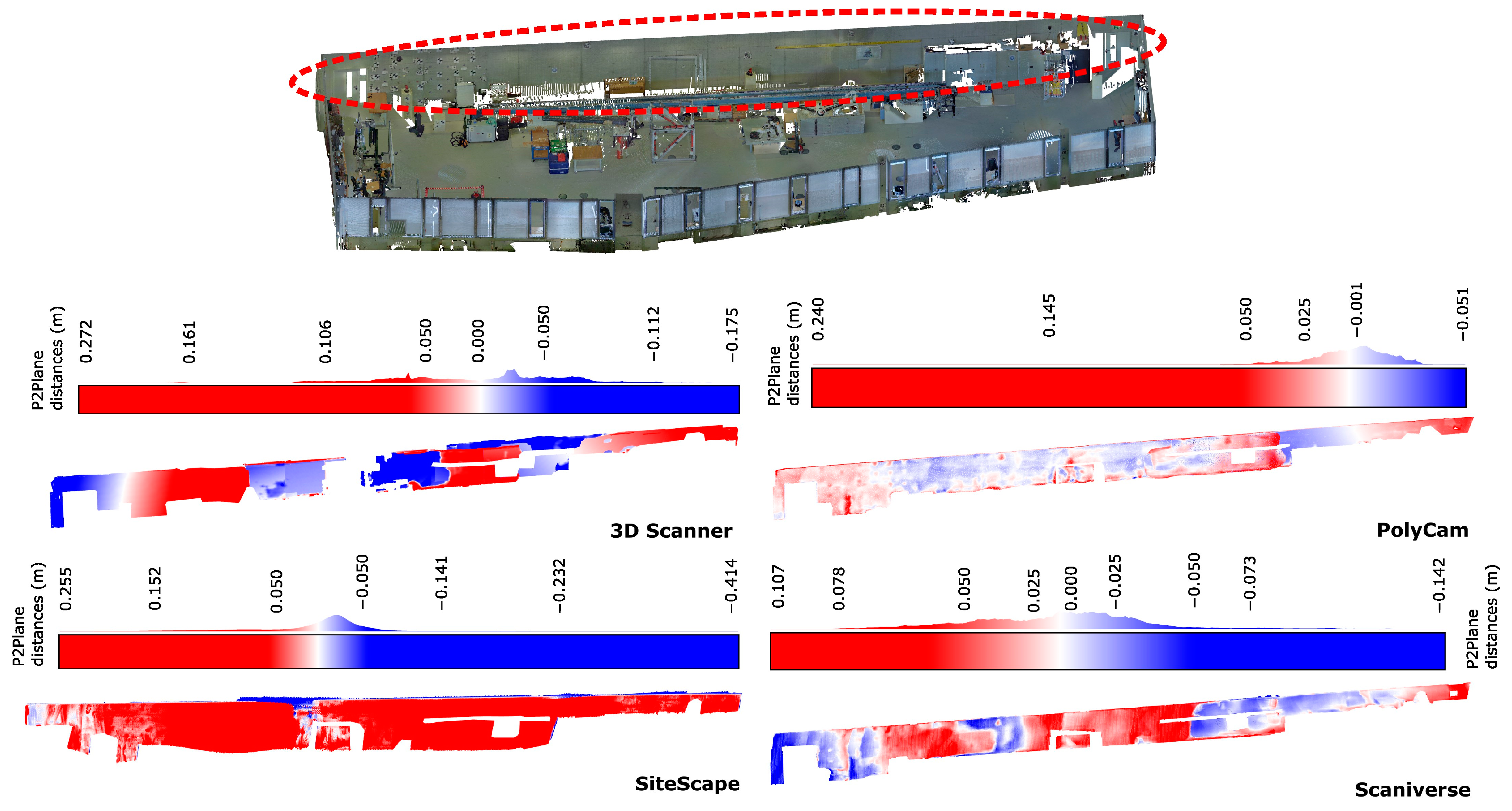
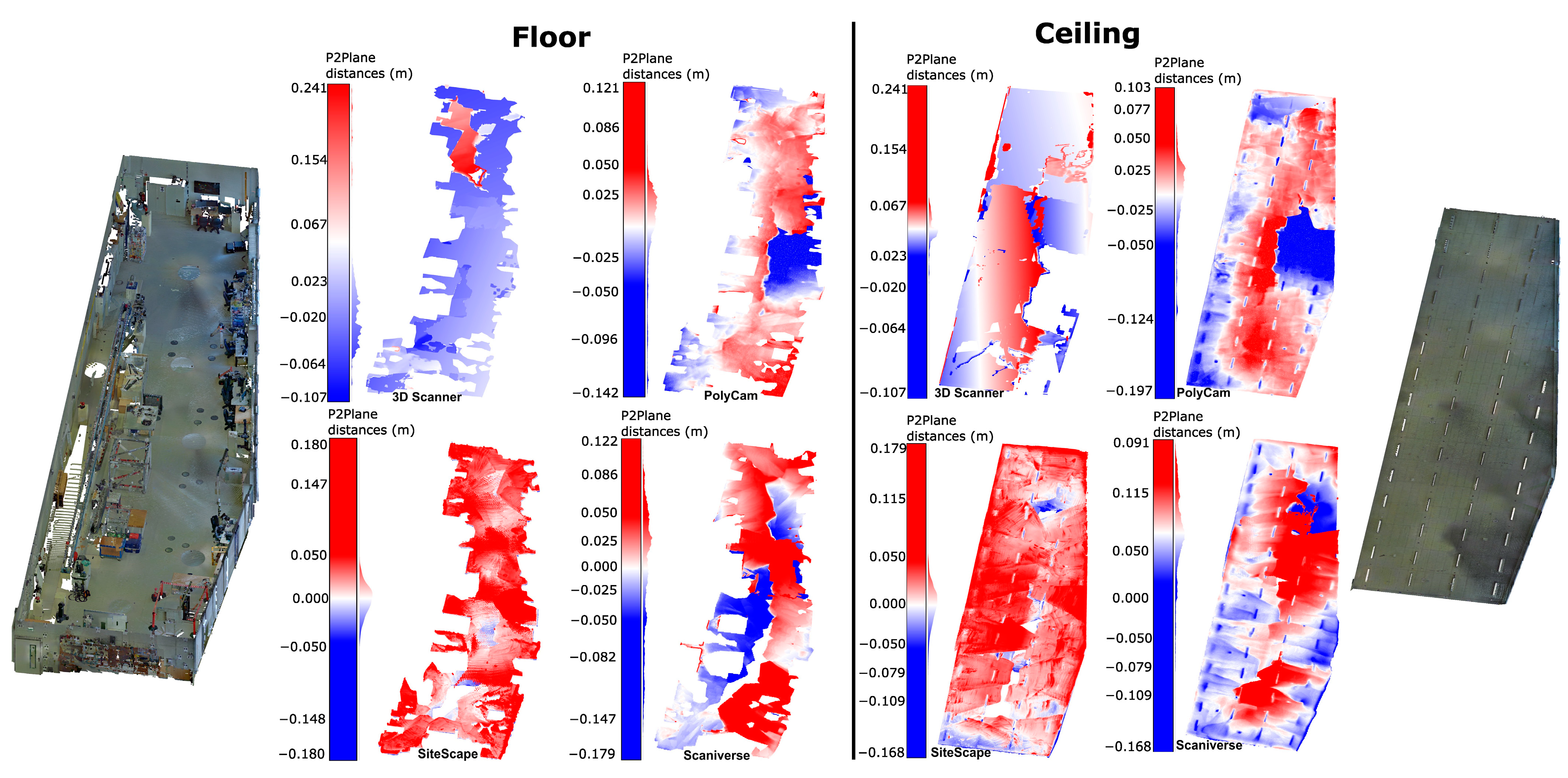
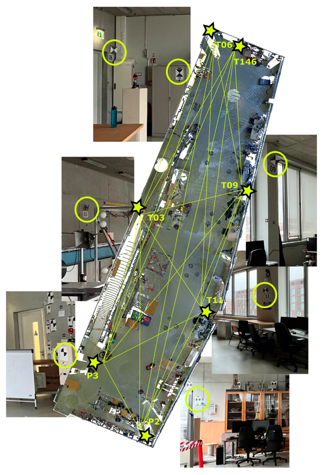
4. Results
5. Discussion and Conclusions
Author Contributions
Funding
Institutional Review Board Statement
Informed Consent Statement
Data Availability Statement
Conflicts of Interest
References
- Di Stefano, F.; Chiappini, S.; Gorreja, A.; Balestra, M.; Pierdicca, R. Mobile 3D scan LiDAR: A literature review. Geomatics Nat. Hazards Risk 2021, 12, 2387–2429. [Google Scholar] [CrossRef]
- Scantech International. Timeline of 3D Laser Scanners | By Scantech International. Available online: https://scantech-international.com/blog/timeline-of-3d-laser-scanners (accessed on 3 March 2023).
- Pritchard, D.; Sperner, J.; Hoepner, S.; Tenschert, R. Terrestrial laser scanning for heritage conservation: The Cologne Cathedral documentation project. ISPRS Ann. Photogramm. Remote Sens. Spat. Inf. Sci. 2017, IV-2/W2, 213. [Google Scholar] [CrossRef]
- Kushwaha, S.K.P.; Dayal, K.R.; Sachchidanand; Raghavendra, S.; Pande, H.; Tiwari, P.S.; Agrawal, S.; Srivastava, S.K. 3D Digital Documentation of a Cultural Heritage Site Using Terrestrial Laser Scanner—A Case Study. In Applications of Geomatics in Civil Engineering, 1st ed.; Lecture Notes in Civil Engineering; Ghosh, J.K., da Silva, I., Eds.; Springer: Singapore, 2020; Volume 33, pp. 49–58. [Google Scholar] [CrossRef]
- Lague, D.; Brodu, N.; Leroux, J. Accurate 3D comparison of complex topography with terrestrial laser scanner: Application to the Rangitikei canyon (N-Z). ISPRS J. Photogramm. Remote Sens. 2013, 82, 10–26. [Google Scholar] [CrossRef]
- Schürch, P.; Densmore, A.L.; Rosser, N.J.; Lim, M.; McArdell, B.W. Detection of surface change in complex topography using terrestrial laser scanning: Application to the Illgraben debris-flow channel. Earth Surf. Process. Landf. 2011, 36, 1847–1859. [Google Scholar] [CrossRef]
- Sternberg, H. Deformation Measurements at Historical Buildings with Terrestrial Laserscanners. In Proceedings of the ISPRS Commission V Symposium Image Engineering and Vision Metrology, Dresden, Germany, 25–27 September 2006; pp. 303–308. Available online: https://www.isprs.org/proceedings/xxxvi/part5/paper/STER_620.pdf (accessed on 17 July 2023).
- Wang, W.; Zhao, W.; Huang, L.; Vimarlund, V.; Wang, Z. Applications of terrestrial laser scanning for tunnels: A review. J. Traffic Transp. Eng. (Eng. Ed.) 2014, 1, 325–337. [Google Scholar] [CrossRef]
- Mukupa, W.; Roberts, G.W.; Hancock, C.M.; Al-Manasir, K. A review of the use of terrestrial laser scanning application for change detection and deformation monitoring of structures. Surv. Rev. 2017, 49, 99–116. [Google Scholar] [CrossRef]
- Raza, M. BIM for Existing Buildings: A Study of Terrestrial Laser Scanning and Conventional Measurement Technique. Master’s Thesis, Metropolia University of Applied Sciences, Helsinki, Finland, 2017. [Google Scholar]
- Park, H.; Lim, S.; Trinder, J.; Turner, R. 3D surface reconstruction of Terrestrial Laser Scanner data for forestry. In Proceedings of the IGARSS 2010–2010 IEEE International Geoscience and Remote Sensing Symposium, Honolulu, HI, USA, 25–30 July 2010; pp. 4366–4369. [Google Scholar]
- Petrie, G. An Introduction to the Technology Mobile Mapping Systems. GeoInformatics 2016, 13, 32–43. Available online: http://petriefied.info/Petrie_Mobile_Mapping_Systems_Jan-Feb_2010.pdf (accessed on 17 July 2023).
- Hamraz, H.; Contreras, M.A.; Zhang, J. Forest understory trees can be segmented accurately within sufficiently dense airborne laser scanning point clouds. Sci. Rep. 2017, 7, 6770. [Google Scholar] [CrossRef]
- Chen, D.; Wang, R.; Peethambaran, J. Topologically Aware Building Rooftop Reconstruction From Airborne Laser Scanning Point Clouds. IEEE Trans. Geosci. Remote Sens. 2017, 55, 7032–7052. [Google Scholar] [CrossRef]
- Toth, C.; Grejner-Brzezinska, D. Redefining the Paradigm of Modern Mobile Mapping. Photogramm. Eng. Remote Sens. 2004, 70, 685–694. [Google Scholar] [CrossRef]
- Briese, C.; Zach, G.; Verhoeven, G.; Ressl, C.; Ullrich, A.; Studnicka, N.; Doneus, M. Analysis of mobile laser scanning data and multi-view image reconstruction. ISPRS-Int. Arch. Photogramm. Remote Sens. Spat. Inf. Sci. 2012, XXXIX-B5, 163–168. [Google Scholar] [CrossRef]
- Stojanovic, V.; Shoushtari, H.; Askar, C.; Scheider, A.; Schuldt, C.; Hellweg, N.; Sternberg, H. A Conceptual Digital Twin for 5G Indoor Navigation. 2021. Available online: https://www.researchgate.net/publication/351234064 (accessed on 30 November 2023).
- Ibrahimkhil, M.H.; Shen, X.; Barati, K.; Wang, C.C. Dynamic Progress Monitoring of Masonry Construction through Mobile SLAM Mapping and As-Built Modeling. Buildings 2023, 13, 930. [Google Scholar] [CrossRef]
- Mahdjoubi, L.; Moobela, C.; Laing, R. Providing real-estate services through the integration of 3D laser scanning and building information modelling. Comput. Ind. 2013, 64, 1272–1281. [Google Scholar] [CrossRef]
- Sgrenzaroli, M.; Barrientos, J.O.; Vassena, G.; Sanchez, A.; Ciribini, A.; Ventura, S.M.; Comai, S. Indoor mobile mapping systems and (bim) digital models for construction progress monitoring. ISPRS-Int. Arch. Photogramm. Remote Sens. Spat. Inf. Sci. 2022, XLIII-B1-2, 121–127. [Google Scholar] [CrossRef]
- Lehtola, V.V.; Nikoohemat, S.; Nüchter, A.; Lehtola, V.V.; Nikoohemat, S.; Nüchter, A. Indoor 3D: Overview on Scanning and Reconstruction Methods. In Handbook of Big Geospatial Data; Werner, M., Chiang, Y.-Y., Eds.; Springer: Berlin, Germany, 2021; pp. 55–97. [Google Scholar] [CrossRef]
- Lachat, E.; Macher, H.; Mittet, M.-A.; Landes, T.; Grussenmeyer, P. First experiences with kinect v2 sensor for close range 3d modelling. ISPRS-Int. Arch. Photogramm. Remote Sens. Spat. Inf. Sci. 2015, XL-5/W4, 93–100. [Google Scholar] [CrossRef]
- Khoshelham, K.; Tran, H.; Acharya, D. Indoor mapping eyewear: Geometric evaluation of spatial mapping capability of hololens. ISPRS-Int. Arch. Photogramm. Remote Sens. Spat. Inf. Sci. 2019, XLII-2/W13, 805–810. [Google Scholar] [CrossRef]
- Delasse, C.; Lafkiri, H.; Hajji, R.; Rached, I.; Landes, T. Indoor 3D Reconstruction of Buildings via Azure Kinect RGB-D Camera. Sensors 2022, 22, 9222. [Google Scholar] [CrossRef]
- Hübner, P.; Clintworth, K.; Liu, Q.; Weinmann, M.; Wursthorn, S. Evaluation of HoloLens Tracking and Depth Sensing for Indoor Mapping Applications. Sensors 2020, 20, 1021. [Google Scholar] [CrossRef]
- Weinmann, M.; Wursthorn, S.; Jutzi, B. Semi-automatic image-based co-registration of range imaging data with different characteristics. ISPRS-Int. Arch. Photogramm. Remote Sens. Spat. Inf. Sci. 2013, XXXVIII-3, 119–124. [Google Scholar] [CrossRef]
- Kalantari, M.; Nechifor, M. 3D Indoor Surveying—A Low Cost Approach. Surv. Rev. 2016, 49, 1–6. [Google Scholar] [CrossRef]
- Lehtola, V.V.; Kaartinen, H.; Nüchter, A.; Kaijaluoto, R.; Kukko, A.; Litkey, P.; Honkavaara, E.; Rosnell, T.; Vaaja, M.T.; Virtanen, J.-P.; et al. Comparison of the Selected State-Of-The-Art 3D Indoor Scanning and Point Cloud Generation Methods. Remote Sens. 2017, 9, 796. [Google Scholar] [CrossRef]
- Tucci, G.; Visintini, D.; Bonora, V.; Parisi, E.I. Examination of Indoor Mobile Mapping Systems in a Diversified Internal/External Test Field. Appl. Sci. 2018, 8, 401. [Google Scholar] [CrossRef]
- di Filippo, A.; Sánchez-Aparicio, L.J.; Barba, S.; Martín-Jiménez, J.A.; Mora, R.; Aguilera, D.G. Use of a Wearable Mobile Laser System in Seamless Indoor 3D Mapping of a Complex Historical Site. Remote Sens. 2018, 10, 1897. [Google Scholar] [CrossRef]
- Salgues, H.; Macher, H.; Landes, T. Evaluation of mobile mapping systems for indoor surveys. ISPRS-Int. Arch. Photogramm. Remote Sens. Spat. Inf. Sci. 2020, XLIV-4/W1-2020, 119–125. [Google Scholar] [CrossRef]
- Wilkening, J.; Kapaj, A.; Cron, J. Creating a 3D Campus Routing Information System with ArcGIS Indoors. In Dreiländertagung der OVG, DGPF und SGPF Photogrammetrie-Fernerkundung-Geoinformation-2019; Thomas Kersten: Hamburg, Germany, 2019. [Google Scholar]
- Murtiyoso, A.; Grussenmeyer, P.; Landes, T.; Macher, H. First assessments into the use of commercial-grade solid state lidar for low cost heritage documentation. ISPRS-Int. Arch. Photogramm. Remote Sens. Spat. Inf. Sci. 2021, XLIII-B2-2, 599–604. [Google Scholar] [CrossRef]
- Shoushtari, H.; Willemsen, T.; Sternberg, H. Many Ways Lead to the Goal—Possibilities of Autonomous and Infrastructure-Based Indoor Positioning. Electronics 2021, 10, 397. [Google Scholar] [CrossRef]
- Tanskanen, P.; Kolev, K.; Meier, L.; Camposeco, F.; Saurer, O.; Pollefeys, M. Live Metric 3D Reconstruction on Mobile Phones. In Proceedings of the 2013 IEEE International Conference on Computer Vision (ICCV), Sydney, Australia, 1–8 December 2013; pp. 65–72. [Google Scholar]
- Kersten, T.P. The Smartphone as a Professional Mapping Tool | GIM International. GIM International, 25 February 2020. Available online: https://www.gim-international.com/content/article/the-smartphone-as-a-professional-mapping-tool (accessed on 17 July 2023).
- Wikipedia. Tango (Platform)-Wikipedia. Available online: https://en.wikipedia.org/wiki/Tango_(platform) (accessed on 10 May 2023).
- Bianchini, C.; Catena, L. The Democratization of 3D Capturing an Application Investigating Google Tang Potentials. Int. J. Bus. Hum. Soc. Sci. 2019, 12, 3298576. [Google Scholar] [CrossRef]
- Google. Build New Augmented Reality Experiences that Seamlessly Blend the Digital and Physical Worlds | ARCore | Google Developers. Available online: https://developers.google.com/ar (accessed on 10 May 2023).
- Diakité, A.A.; Zlatanova, S. First experiments with the tango tablet for indoor scanning. ISPRS Ann. Photogramm. Remote Sens. Spat. Inf. Sci. 2016, III-4, 67–72. [Google Scholar] [CrossRef]
- Froehlich, M.; Azhar, S.; Vanture, M. An Investigation of Google Tango® Tablet for Low Cost 3D Scanning. In Proceedings of the 34th International Symposium on Automation and Robotics in Construction, Taipei, Taiwan, 28 June–1 July 2017; pp. 864–871. [Google Scholar]
- Boboc, R.G.; Gîrbacia, F.; Postelnicu, C.C.; Gîrbacia, T. Evaluation of Using Mobile Devices for 3D Reconstruction of Cultural Heritage Artifacts. In VR Technologies in Cultural Heritage; Duguleană, M., Carrozzino, M., Gams, M., Tanea, I., Eds.; Communications in Computer and Information Science; Springer International Publishing: Cham, Swizterland, 2019; Volume 904, pp. 46–59. [Google Scholar] [CrossRef]
- Luetzenburg, G.; Kroon, A.; Bjørk, A.A. Evaluation of the Apple iPhone 12 Pro LiDAR for an Application in Geosciences. Sci. Rep. 2021, 11, 1–9. [Google Scholar] [CrossRef]
- Riquelme, A.; Tomás, R.; Cano, M.; Pastor, J.L.; Jordá-Bordehore, L. Extraction of discontinuity sets of rocky slopes using iPhone-12 derived 3DPC and comparison to TLS and SfM datasets. IOP Conf. Ser. Earth Environ. Sci. 2021, 833, 012056. [Google Scholar] [CrossRef]
- Losè, L.T.; Spreafico, A.; Chiabrando, F.; Tonolo, F.G. Apple LiDAR Sensor for 3D Surveying: Tests and Results in the Cultural Heritage Domain. Remote Sens. 2022, 14, 4157. [Google Scholar] [CrossRef]
- Díaz-Vilariño, L.; Tran, H.; Frías, E.; Balado, J.; Khoshelham, K. 3D mapping of indoor and outdoor environments using Apple smart devices. ISPRS-Int. Arch. Photogramm. Remote Sens. Spat. Inf. Sci. 2022, XLIII-B4-2, 303–308. [Google Scholar] [CrossRef]
- Spreafico, A.; Chiabrando, F.; Losè, L.T.; Tonolo, F.G. The ipad pro built-in lidar sensor: 3D rapid mapping tests and quality assessment. ISPRS-Int. Arch. Photogramm. Remote Sens. Spat. Inf. Sci. 2021, XLIII-B1-2, 63–69. [Google Scholar] [CrossRef]
- Zoller+Fröhlich. Z+F IMAGER® 5016: Zoller+Fröhlich. Available online: https://www.zofre.de/laserscanner/3d-laserscanner/z-f-imagerr-5016 (accessed on 17 July 2023).
- CloudCompare. (version. 2.12.4) [GPL Software]. Available online: http://www.cloudcompare.org/ (accessed on 14 July 2022).
- U.S. Institute of Building Documentation. USIBD Level of Accuracy (LOA) Specification Guide, v2.0-2016. 2016. Available online: https://cdn.ymaws.com/www.nysapls.org/resource/resmgr/2019_conference/handouts/hale-g_bim_loa_guide_c120_v2.pdf (accessed on 12 October 2022).
- Schnabel, R.; Wahl, R.; Klein, R. Efficient RANSAC for point-cloud shape detection. In Proceedings of the 2007 Computer Graphics Forum, Honolulu, HI, USA, 25–29 June 2017; pp. 214–226. [Google Scholar] [CrossRef]


| 3D Scanner App | PolyCam | SiteScape | Scaniverse | |
|---|---|---|---|---|
| Scan mode | LIDAR, LIDAR Advance, Point Cloud, Photos, TrueDepth | LIDAR, Photo, Room | LIDAR | Small object, medium object, large object (area) |
| Scan settings | Resolution, max depth | - | Point density and size (low, med, high) | Range setting (max 5 m) |
| Processing options | HD, Fast, Custom | Fast, Space, Object, Custom | Synching to the SiteScape cloud | Speed, area, detail |
| Processing steps | Smoothing, simplifying, texturing | - | - | - |
| Export as | Point cloud, mesh | Point cloud, mesh | Point cloud | Point cloud, mesh |
| Export formats | PCD, PLY, LAS, e57, PTS, XYZ, OBJ, KMZ, FBX etc. | DXF, PLY, LAS, PTS, XYZ, OBJ, STL, FBX etc. | e57 | PLY, LAS, OBJ, FBX, STL, GLB, USDZ |
| 3D Scanner App | PolyCam | SiteScape | Scaniverse | |
|---|---|---|---|---|
| <5 mm | 17% | 19% | 8% | 10% |
| 5 mm–1 cm | 11% | 17% | 10% | 10% |
| 1–3 cm | 30% | 32% | 46% | 31% |
| 3–5 cm | 11% | 9% | 19% | 19% |
| 5–10 cm | 12% | 9% | 9% | 18% |
| 10–20 cm | 11% | 12% | 6% | 9% |
| 20–40 cm | 8% | 2% | 2% | 3% |
| Std (cm) | 9 | 7 | 6 | 8 |
| Level | Upper Range | Lower Range |
|---|---|---|
| LOA10 | User-defined | 5 cm |
| LOA20 | 5 cm | 15 mm |
| LOA30 | 15 mm | 5 mm |
| LOA40 | 5 mm | 1 mm |
| LOA50 | 1 mm | 0 |
| 3DScanner | PolyCam | SiteScape | Scaniverse | |||||||||
|---|---|---|---|---|---|---|---|---|---|---|---|---|
| Floor | Ceiling | Wall | Floor | Ceiling | Wall | Floor | Ceiling | Wall | Floor | Ceiling | Wall | |
| <1 cm | 21% | 38% | 8% | 27% | 27% | 44% | 45% | 37% | 18% | 13% | 28% | 24% |
| 1–3 cm | 34% | 40% | 27% | 44% | 47% | 46% | 45% | 48% | 35% | 26% | 32% | 43% |
| 3–5 cm | 29% | 14% | 24% | 17% | 16% | 8% | 8% | 12% | 17% | 24% | 19% | 19% |
| 5–10 cm | 9% | 5% | 33% | 8% | 7% | 1% | 1% | 3% | 17% | 29% | 20% | 12% |
| >10 cm | 7% | 2% | 7% | 4% | 4% | 0% | 0% | 0% | 12% | 8% | 2% | 1% |
| Std (cm) | 5.7 | 3.5 | 5.7 | 3.8 | 3.5 | 1.9 | 2.0 | 2.2 | 6.5 | 5.5 | 4.0 | 3.4 |
| TLS | 3D Scanner App | PolyCam | SiteScape | Scaniverse | |||||||||||
|---|---|---|---|---|---|---|---|---|---|---|---|---|---|---|---|
| Points | X | Y | Z | X | Y | Z | X | Y | Z | X | Y | Z | X | Y | Z |
| P1 | 1.399 | −4.199 | −1.127 | 1.402 | −4.183 | −1.097 | 1.406 | −4.043 | −1.135 | 1.356 | −4.108 | −1.095 | - | - | - |
| P2 | 8.464 | −4.221 | −0.703 | 8.301 | −4.074 | −0.708 | 8.452 | −4.091 | −0.690 | 8.452 | −4.059 | −0.671 | 8.131 | −3.531 | −0.678 |
| P3 | 0.669 | −0.602 | −0.968 | 0.674 | −0.602 | −0.965 | 0.675 | −0.465 | −0.984 | 0.686 | −0.649 | −0.918 | 0.648 | 0.379 | −0.989 |
| T03 | 0.002 | 14.021 | 0.012 | −0.132 | 13.838 | −0.013 | −0.095 | 13.986 | 0.040 | 0.055 | 14.042 | 0.068 | −0.029 | 14.377 | 0.033 |
| T04 | 0.007 | 18.441 | 0.953 | - | - | - | −0.072 | 18.364 | 0.982 | 0.098 | 18.370 | 1.057 | −0.105 | 18.648 | 0.058 |
| T06 | 0.024 | 30.649 | 0.267 | 0.099 | 30.587 | 0.045 | 0.022 | 30.632 | 0.297 | 0.042 | 30.615 | 0.309 | 0.037 | 30.615 | 0.258 |
| T08 | 6.771 | 27.013 | −1.939 | 6.816 | 27.048 | −1.919 | 6.828 | 26.964 | −1.946 | 6.675 | 27.330 | −1.907 | - | - | - |
| T09 | 7.950 | 19.152 | 0.882 | 8.008 | 19.205 | 0.914 | 8.002 | 19.312 | 0.921 | 7.919 | 19.163 | 0.853 | - | - | - |
| T11 | 9.524 | 8.143 | −0.043 | 9.438 | 8.066 | 0.032 | 9.630 | 8.141 | −0.036 | 9.503 | 7.983 | 0.036 | 9.599 | 8.245 | −0.195 |
| T13 | 8.731 | −4.133 | 0.107 | - | - | - | 8.705 | −4.086 | 0.144 | 8.679 | −4.027 | 0.113 | 8.394 | −3.528 | 0.181 |
| T146 | 1.974 | 30.446 | −0.413 | 2.099 | 30.413 | −0.276 | 2.003 | 30.431 | −0.413 | 2.000 | 30.385 | −0.427 | 1.965 | 30.444 | −0.360 |
| Distances (m) | TLS (d_{TLS}) | 3D Scanner (d_{3D}) | PolyCam (d_{P}) | SiteScape (d_{SI}) | Scaniverse (d_{SC}) | d_{TLS}-d_{3D} | d_{TLS}-d_{P} | d_{TLS}-d_{SI} | d_{TLS}-d_{SC} |
|---|---|---|---|---|---|---|---|---|---|
| P2–P3 | 8.599 | 8.384 | 8.586 | 8.485 | 8.449 | 0.215 | 0.013 | 0.113 | 0.150 |
| P2–T03 | 20.122 | 19.810 | 20.009 | 19.968 | 19.692 | 0.312 | 0.113 | 0.154 | 0.429 |
| P2–T06 | 35.890 | 35.626 | 35.745 | 35.693 | 35.105 | 0.264 | 0.145 | 0.198 | 0.786 |
| P2–T11 | 12.427 | 12.216 | 12.306 | 12.108 | 11.877 | 0.211 | 0.121 | 0.318 | 0.550 |
| P2–T146 | 35.270 | 35.043 | 35.120 | 35.044 | 34.531 | 0.228 | 0.150 | 0.227 | 0.739 |
| P3–T03 | 14.671 | 14.494 | 14.508 | 14.738 | 14.052 | 0.177 | 0.163 | −0.066 | 0.620 |
| P3–T06 | 31.283 | 31.211 | 31.130 | 31.295 | 30.268 | 0.072 | 0.152 | −0.012 | 1.015 |
| P3–T11 | 12.480 | 12.367 | 12.456 | 12.376 | 11.943 | 0.113 | 0.024 | 0.104 | 0.537 |
| P3–T146 | 31.081 | 31.055 | 30.930 | 31.066 | 30.100 | 0.025 | 0.151 | 0.015 | 0.980 |
| T03–T06 | 16.630 | 16.751 | 16.648 | 16.575 | 16.240 | −0.120 | −0.018 | 0.056 | 0.391 |
| T03–T11 | 11.190 | 11.176 | 11.347 | 11.224 | 11.417 | 0.014 | −0.157 | −0.034 | −0.227 |
| T03–T146 | 16.548 | 16.727 | 16.584 | 16.466 | 16.195 | −0.178 | −0.036 | 0.083 | 0.353 |
| T06–T11 | 24.431 | 24.381 | 24.460 | 24.531 | 24.332 | 0.051 | −0.028 | −0.100 | 0.099 |
| T06–T146 | 2.075 | 2.033 | 2.114 | 2.104 | 2.032 | 0.042 | −0.039 | −0.029 | 0.044 |
| T11–T146 | 23.549 | 23.523 | 23.562 | 23.630 | 23.476 | 0.026 | −0.013 | −0.080 | 0.074 |
| Mean (m) | 0.097 | 0.049 | 0.063 | 0.436 | |||||
| RMSE (m) | 0.166 | 0.107 | 0.135 | 0.559 | |||||
| Mean and RMSE values calculated after excluding P2. | Mean (m) | 0.022 | 0.020 | −0.007 | 0.388 | ||||
| RMSE (m) | 0.101 | 0.101 | 0.066 | 0.549 | |||||
Disclaimer/Publisher’s Note: The statements, opinions and data contained in all publications are solely those of the individual author(s) and contributor(s) and not of MDPI and/or the editor(s). MDPI and/or the editor(s) disclaim responsibility for any injury to people or property resulting from any ideas, methods, instructions or products referred to in the content. |
© 2023 by the authors. Licensee MDPI, Basel, Switzerland. This article is an open access article distributed under the terms and conditions of the Creative Commons Attribution (CC BY) license (https://creativecommons.org/licenses/by/4.0/).
Share and Cite
Askar, C.; Sternberg, H. Use of Smartphone Lidar Technology for Low-Cost 3D Building Documentation with iPhone 13 Pro: A Comparative Analysis of Mobile Scanning Applications. Geomatics 2023, 3, 563-579. https://doi.org/10.3390/geomatics3040030
Askar C, Sternberg H. Use of Smartphone Lidar Technology for Low-Cost 3D Building Documentation with iPhone 13 Pro: A Comparative Analysis of Mobile Scanning Applications. Geomatics. 2023; 3(4):563-579. https://doi.org/10.3390/geomatics3040030
Chicago/Turabian StyleAskar, Cigdem, and Harald Sternberg. 2023. "Use of Smartphone Lidar Technology for Low-Cost 3D Building Documentation with iPhone 13 Pro: A Comparative Analysis of Mobile Scanning Applications" Geomatics 3, no. 4: 563-579. https://doi.org/10.3390/geomatics3040030