Automated Modeling of Road Networks for High-Definition Maps in OpenDRIVE Format Using Mobile Mapping Measurements

Abstract

With growing attention being devoted to autonomous vehicle (AV) safety, people have recently attached importance to high-definition (HD) maps. HD maps are not limited by environmental factors and can limit AVs driving in certain lanes. HD maps provide accurate auxiliary information on factors such as road geometry, traffic sign placement, and traffic topology. Nowadays, most HD maps are made from point clouds data, and this data contains accurate 3D position information. However, the production costs associated with HD maps are substantial. This article proposes an algorithm that reduces a great amount of time and human resource. The algorithm is divided into three phases, lane lines’ extraction from point clouds, modelling lane lines with attributes, and building OpenDRIVE file. The algorithm extracts lane lines resting on intensity value within the range of roads. Next, it models lane lines by cubic spline interpolation with the result of first phase, and build the OpenDRIVE file following the announcement of OpenDRIVE. The final result is compared with the verified HD map from the mapping company to analyze the accuracy. The root mean square (RMSE) obtained were 0.069 and 0.079 m for 2D and 3D maps, respectively.

1. Background

Maps such as Google Maps are designed for interpretation by humans and not autonomous vehicles (AVs). A primary task related to high-definition (HD) maps is ensuring that map information can be transferred to and be recognized by AVs such that these vehicles can plan journeys similar to how humans do [1]. In HD maps, traffic information must be precise to achieve AV safety [2]. Many HD map formats are available, with the main ones being Autoware Vector Map, OpenDRIVE, Lanelet2, and Navigation Data Standard (NDS). Autoware Vector Map contains many thematical comma-separated value (CSV) files, and 32 types of .csv file provide road information in Autoware Vector Map format [1]. OpenDRIVE is mainly used for simulation-based applications; it is an open-source format organized in a hierarchical structure and compiled in Extensible Markup Language (XML). OpenDRIVE describes true road geometric properties and contains one reference line and lanes that are built around the reference line [1]. The use of NDS is standard among automotive companies, map data producers, and manufacturers of navigation devices, but it is not a fully open-source format [1]. Lanelet2 maps use six primitives to describe all map data. The utility of HD maps extends far beyond isolated applications such as localization or motion planning [1]. A comparison of these four map formats is presented in

Table 1. Comparison of HD map formats based on various criteria which is adapted from [1].

Criteria	OpenDRIVE	Autoware Vector Map	Lanelet2	NDS
Ease of Creation	1	3	4	2
Applications	4	3	3	4
Adoption of Format	4	1	2	5
Expressiveness	4	2	3	5
Accessibility	4	2	5	1
Total	17	11	17	17

, and each format is rated according to different criteria [1]. Table 1. reveals that the best map formats are NDS, Lanelet2, and OpenDRIVE.

According to [3] and the official NDS website, NDS is a standardized format for automotive-grade navigation databases, but it is not an open-source format. Since its use requires the purchase of a license, this format is not ideal for academic research. As indicated in Table 1, NDS exhibits excellent performance in adoption and expressiveness. It was originally created for use by major automotive companies; thus, it has the highest level of integration of all map formats. However, due to NDS’s requirement that a license is purchased, it is not widely used by laypersons.

Lanelet2 is an HD map format with high accessibility, as indicated in [3]. Lanelet2 format should be used for two simple reasons: it is an open-source format and can hold more information than other formats. It describes road information based on various factors and atomic lane sections and consists of different layers [4]. Lanelets, which are atomic lane sections, are related to each other, and Lanelet2 presents lane topologies in a simple manner. As indicated in [3], Lanelet2 divides the roads into a hierarchical structure of six primitives, namely points, linestrings, polygons, lanelets, areas, and regulatory elements. Lanelet2 provides different types of information through these six layers. The hierarchical representation of abundant traffic information is efficient. Lanelet2 seems to be the most suitable format for use by researchers and laypersons, but it was developed more recently than other HD map formats. Moreover, some problems related to adoption must be solved; therefore, this format was not the optimal choice for use in this study.

2. Introduction

Besides NDS and Lanelet2, OpenDRIVE is the most common HD map format. Owing to the restriction of NDS and Lanelet2, the requirement of license in NDS and low adoption of Lanelet2, OpenDRIVE is selected HD map format in this study. OpenDRIVE has advantages in application, adoption, expressiveness, and accessibility, as shown in Table 1. As long as people can deal with the complexity of creation, OpenDRIVE will likely become the most common HD map format.

A standard format should be created to increase the convenience for the exchange of information using different HD map formats. According to [5], OpenDRIVE should be the standard HD map format used. OpenDRIVE describes the physical relationships between road networks and road objects. It emphasizes the geometric properties of reference lines and the topologies of lanes. Furthermore, road objects, such as traffic signs, barriers, and sidewalks, are individually described in detail. OpenDRIVE maps can be easily checked and editing, which enhances its interoperability. 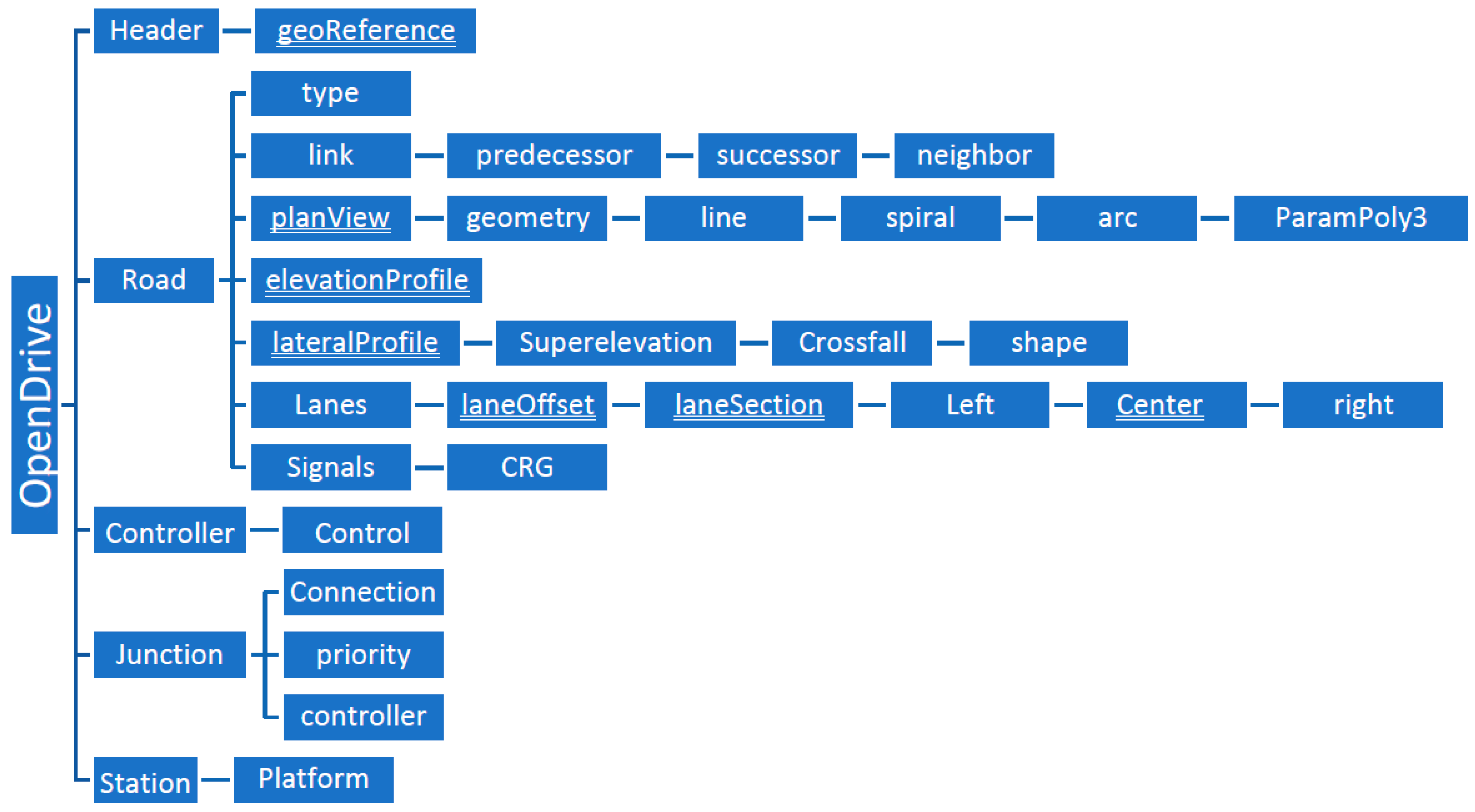One advantage of this format is that it can be easily converted to other HD map formats such as Autoware Vector Map and Lanelet2 [6]. Due to these benefits, OpenDRIVE is the most appropriate HD map format for investigation in this study. The structure of this format is illustrated in Figure 1. OpenDRIVE is compiled using XML, and anyone can edit such maps or even create a fictious HD map using this format. The main components are the header, road elements, controller, junction, and station construct [7]. The OpenDRIVE format is as shown below—Figure 1 illustrates the predefined hierarchy of each main component in OpenDRIVE [8]. This study focused on the establishment of a road segment, and it only retained planView, elevationProfile, lane parts without links (connections), and lateral profiles and signals.

The first component, namely header, describes basic information, such as the production date of OpenDRIVE file, the name of the database and companies, the version of OpenDRIVE, and coordinate projection information [7]. This component provides background information that does not markedly affect map operations; such information can be easily edited.

Road elements, which are the main focus of this study, mainly describe the structure of roads based on reference lines, lanes, and features. OpenDRIVE maps are constructed using reference lines, which present the shapes of roads. These reference lines are coordinates in a reference line system (s and t coordinates), and the s coordinate represents the distance along with the reference line in meters. The t coordinate represents a lane and determines which side of the road it is on. For example, if the t coordinate is negative, the related vehicle is in the right lane.

Four types of geometries are used for simulating reference lines that fit various road scenes, namely line, spiral, arc, and paramPoly3, (parametric cubic curves); another geometry type is used, namely poly3 (cubic polynomial), as illustrated in [8]. Further details are provided in the Methodology section. A pertinent issue related to HD maps is elevation; OpenDRIVE uses a cubic polynomial to fit the elevation of a reference line. Some residuals remain in the cubic polynomial; therefore, it cannot truly represent vertical information.

The width, ID, and attribute of lanes were considered, but the connections between lanes were ignored in this study. Lane ID is based on a t coordinate. Lane ID is an integer, and the shorter the distance is between a reference line and a lane, the lower the absolute lane ID value is. Lane width is represented as a cubic polynomial. Residuals may persist due to the existence of diverse lane shapes; therefore, a lane is divided into sections. This strategy can reduce the residuals in distinct lane shapes within one lane.

The main purpose of this study was to generate HD maps of roads using point cloud data; the result of lane line extraction would determine the accuracy of such maps. The first goal was to determine the road region; ground points had to be retained, and road surface characteristics had to be identified. Some methods were available for achieving such goals, and the mainstream road surface extraction method was based on curb structure, which revealed the height difference between sidewalks and roads [9]. 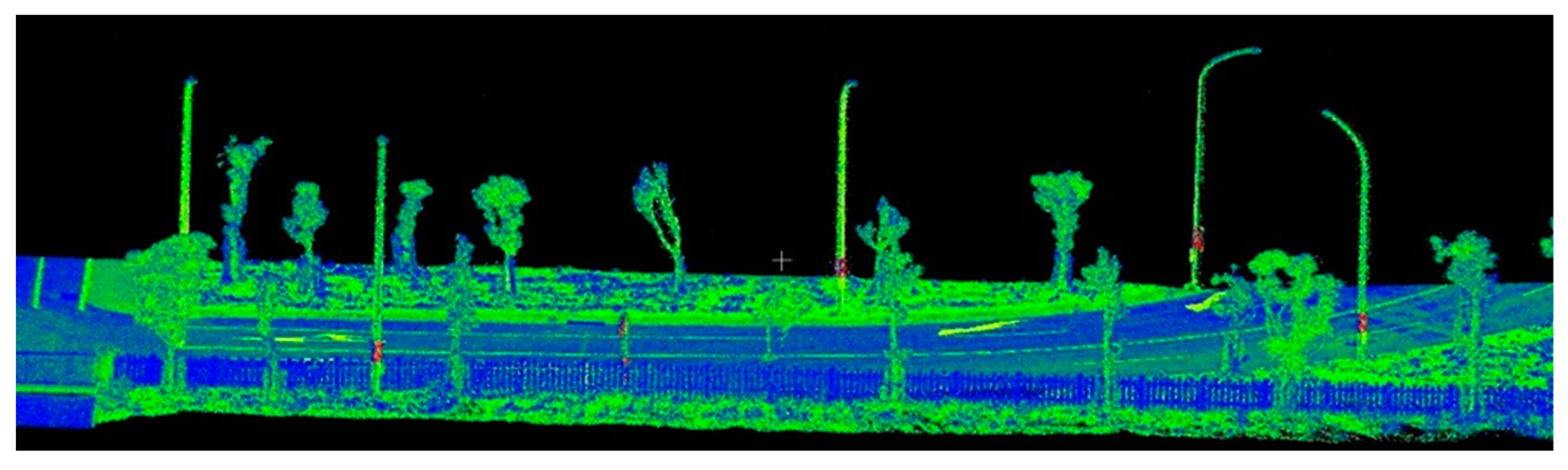A method for distinguishing road surface regions based on the removal of nonground points and road edge detection was proposed in [10]. For the removal of nonground points, a voxel-based upward growing algorithm was used to define nonground points and remove them. In road edge detection, data were segmented, curbs were detected, and finally, road edges were refined by random sample consensus to obtain road surface information. However, the experimental field did not contain curb structures, as indicated in Figure 2. Instead, curbs were adopted as a road extraction condition; therefore, alternative extraction methods for the range of roads were applied. A method for overcoming the problem of an environment not having a curb structure was developed in [11]. Three steps were applied for road surface extraction, namely local road patch extraction, GPBM-based local road surface model estimation, and clustering-based false detection filtering. According to [12], the difference in intensity between point cloud of roads and sidewalks was used to extract road edge information; however, if road boundaries contained material such as dirt, some mistakes may have been made during extraction.

According to [13], a cubic spline could be fitted to a series of points through data interpolation. This approach is useful for approximating a smooth equation, as in Equation (1) the adoption of cubic spline fitting for modeling is a reasonable approach.

fi(x) = ai(x − xi)3 + bi(x − xi)2 + ci(x − xi) + di

(1)

with the modelling of lane lines, the next step was to analyze how polyline data can be modeled in OpenDRIVE format. As indicated in [14], a road could be separated into several segments by using four types of geometry employed in OpenDRIVE, namely lines, spirals, arcs, and polynomials. Moreover, the approach for identifying each type of geometry was the same as that in [14], which was based on curvature features. The main differences between the present study and that study related to measurement data and the representation of the polynomial functions. The measurement data in [14] were obtained from OpenStreetMap, and only horizontal information was retained. As a result, 3D information could not be implemented for elevationProfile and crossfall parts in OpenDRIVE. In addition, in an OpenDRIVE version update, the cubic polynomial was replaced with parametric cubic curves to represent the polynomial function.

3. Materials and Methods

The study is divided into three parts, namely lane line extraction using point clouds, polyline modeling from extraction, and road modeling in OpenDRIVE.

3.1. Lane Line Extraction Using Point Clouds

The methodology described herein improves the detection of road edges through a region growing algorithm; the study flowchart is presented in Figure 3. In the flowchart, the blue parts represent imported data, the green parts represent the algorithm used, the yellow parts represent the results after one phase, and the final results are presented in the orange box. Unprocessed point cloud data are imported, and the trajectory of MLS is used as supporting data. To reduce the capacity required for data processing, absolute coordinates were translated to local coordinates, and down-sampling was applied. After preprocessing, a cloth simulation filter (CSF) was introduced to obtain the ground point clouds in the extraction algorithm. The filter can simulate a ground surface to filter out nonground points not meeting a certain height threshold. The remaining data, namely ground points, are divided into low- and high-intensity data sets by the intensity filter, which clusters the point cloud by intensity value. In the high-intensity data set, point clouds of sidewalks are retained, and it cannot recognize road markings from a high-intensity data set using only an intensity filter.

Road edge extraction is essential for the performance of lane lines extraction. Owing to the lack of a curb structure in the experimental field, region growing was used for road surface clustering to obtain road edge information. In the low-intensity data set containing road surface data, the algorithm takes height value as a condition for region growing. After the extraction of road edges, the road surface region is obtained using a statistical outlier removal filter and the simulated ground surface to identify the point cloud of road markings. The point clouds of these road markings are in disorder; therefore, they are classified as stop lines, arrows, and lane lines through Euclidean distance and oriented bounding box classification. In this study, only the production of lane lines was addressed; the point clouds of lane lines were refined to be imported in the study model.

3.2. Polyline Extraction Model

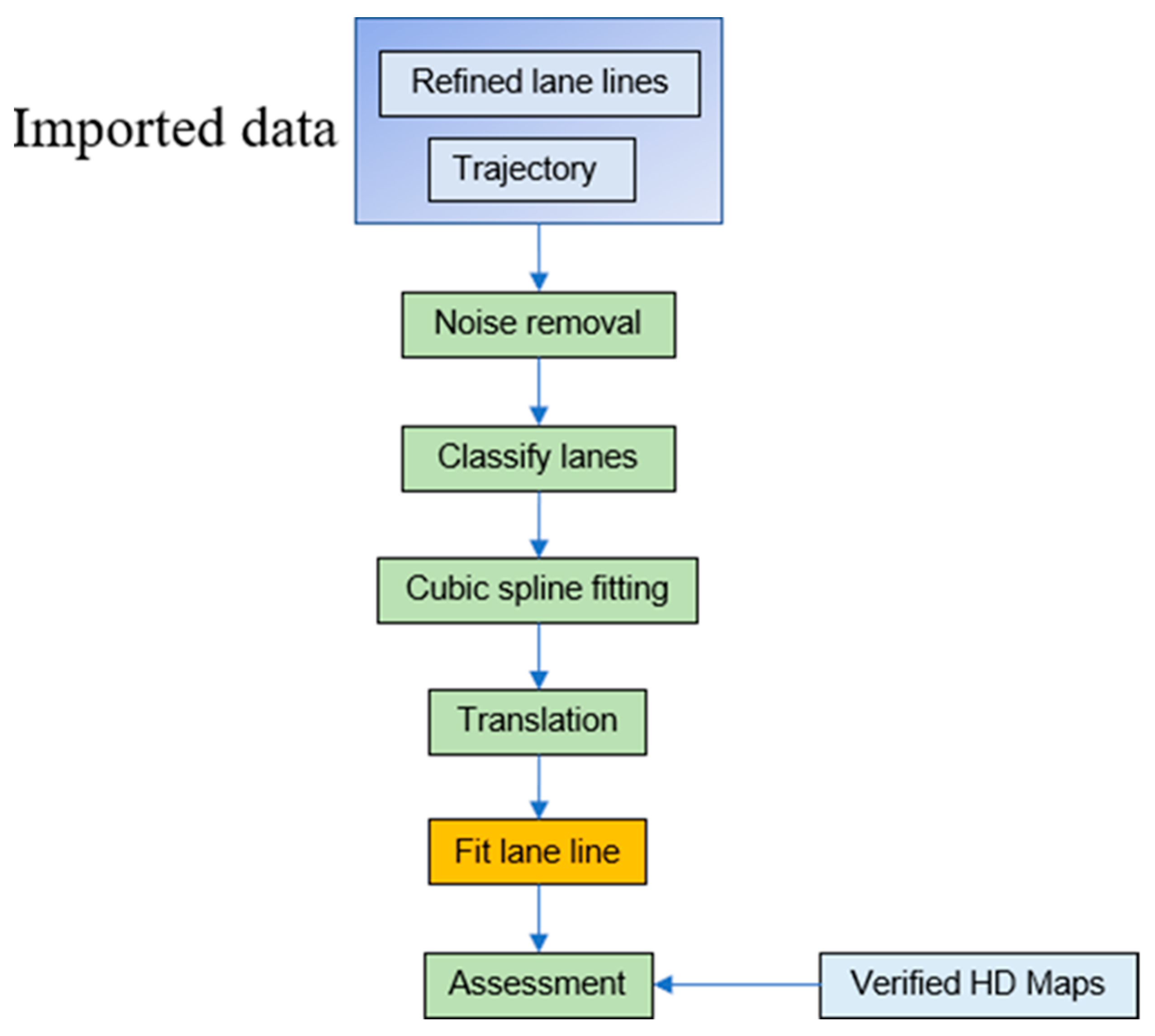
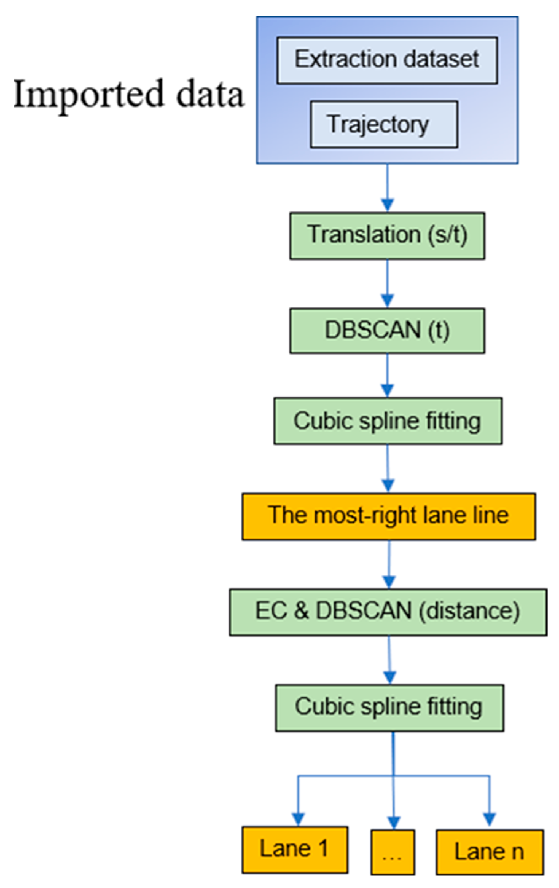
After refined lane line–related point clouds are imported and noise is removed, the algorithm applies cubic spline fitting to generate lane lines with a distance of approximately 10 cm between each point. The algorithm for modeling polylines, as presented in Figure 4, can automatically model lane lines. Classification was applied for data extraction, and the results were assessed, as illustrated in Figure 5.

The first step of modeling polylines after preprocessing is to classify extracted lane lines. The relevant data sets have not been defined with attributes for determining which lanes belonging to. Consequently, the extracted lane lines are first translated into a reference line system, and the original point is the first point of each segmental trajectory; the classification approach is mainly based on such trajectories. In a reference line system (s and t coordinates), the algorithm compares the mean value of the t coordinate from the first to fifth point of each data set to search for the lane line farthest to the right of roads. All data sets are placed in different t coordinate clusters through density-based spatial clustering of applications with noise (DBSCAN). The reason for using DBSCAN is that we cannot confirm the number of lane lines; one advantage of DBSCAN is that unlike K-means clustering, it does not need to define the number of clusters. The minimum cluster is set as the lane line on the far right within these clusters. Afterwards, we must reveal which data sets represent the lane line on the far right, and cubic spline fitting is then applied to fit these data sets.

If the lane line on the far right is derived successfully, the remaining data sets can be classified into the different lane lines to which they belong through Euclidean distance. In accordance with traffic-based logic, all points on each lane line should be the same distance from the lane line on the far right. When this is ensured, DBSCAN is used to classify the points again. The algorithm applies cubic spine fitting to each lane line with a distance of approximately 10 cm between each point. Roads that meet at a junction must be modeled through b-spline fitting as the centroid of intersection due to the lack of lane lines at junctions. Since road marking extraction data are not available at junctions, the modeled lane lines are not as accurate as those for general roads. The resulting maps were compared with the HD maps of reputable mapping companies.

Through Euclidean distance calculation, the algorithm calculates the shortest distance from each point in the results to the points on verified HD maps to analyze the results of polyline modeling.

3.3. Road Modeling Using OpenDRIVE

3.3.1. Geometric Parameters of Reference Lines

The primary goal of analyzing the geometries in the study was to obtain the curvature of each reference line and define each reference line’s geometric properties. The functions of curvature calculations and the intervals of i and j are presented in Equations (2) and (3). curv(i) represents the curvature of every three points, and curv(j) is the mean value of every three curvatures. Averaging was conducted using Equation (3) to avoid the effects of outliers and decrease the model’s computational complexity without losing the characteristics of reference lines after the three-curvature approach was applied.

$$curv\left(i\right)=\frac{\ddot{\stackrel{\rightharpoonup }{\gamma }}\times \dot{\stackrel{\rightharpoonup }{\gamma }}}{\dot{\stackrel{\rightharpoonup }{{\left|\gamma \right|}^3}}}=\frac{x^{″}{y}^{\prime }-x^{\prime }{y}^{″}}{{\left({x^{\prime }}^2+{y^{\prime }}^2\right)}^{\frac{3}{2}}}\hspace{1em}i=1:\left(numbes of points in reference line\right)-2$$

(2)

$$curv\left(j\right)=\frac{{{\displaystyle \sum }}_{n=1}^{3}curv\left(4\times j-n\right)}{3}\hspace{1em}j=1:\left(i÷4\right)$$

(3)

As long as the curvatures are calculated, the reference lines can be segmented into four geometry types based on curvature features. The following section describes the characteristics and the XML structure of each geometry type. The jointly owned geometric parameters of each geometry type are s coordinates (m) at the start position of a road, the start position of x (m) and y (m) in inertial coordinates, the start orientation (hdg) (rad) in inertial coordinates, and the length (m) of segmented reference lines [8]. The definition of s coordinate is that the direction is the tangent of the reference line, and the first s-value is 0. The x and y coordinates are the positions of the first point, and hdg is obtained from the arctangent value of the first two points in inertial coordinates.

• Line:
  The curvature of a line is 0. A line may lose this characteristic if a segment of a reference line is presented as a line in OpenDRIVE format. Consequently, this geometry has to be thoroughly examined if the segment belongs to a line part. A related example is presented as follows: The threshold of a line’s curvature is 0.001, which means that a particular geometry is a line if its curvature value is lower than 0.001. The length of each curvature is approximately 0.4 (m), and the radius of the line is at least 1000 (m); therefore, this threshold is sufficient to rely on due to the huge disparity of the radius of line definition in this part and the length of each curvature. This huge disparity allows ignoring the loss of characteristic.
• Spiral:
  A spiral is a clothoid geometry that describes a part of a reference line with a linear curvature; as such, ∆curvature in Equation (4) is a constant. A spiral is characterized by curvature at the first (curvStart) and last (curvEnd) points.

  ∆curvature = curvature(j + 1) − curvature(j)

  (4)
• Arc:
  An arc exhibits a constant curvature. We do not take arcs to represent all segments of reference lines since the resulting file would be too large to conveniently transfer if all curvatures were presented. Furthermore, achieving an extremely high accuracy of approximately 0.1 cm in the final results is unnecessary.
• Polynomial:
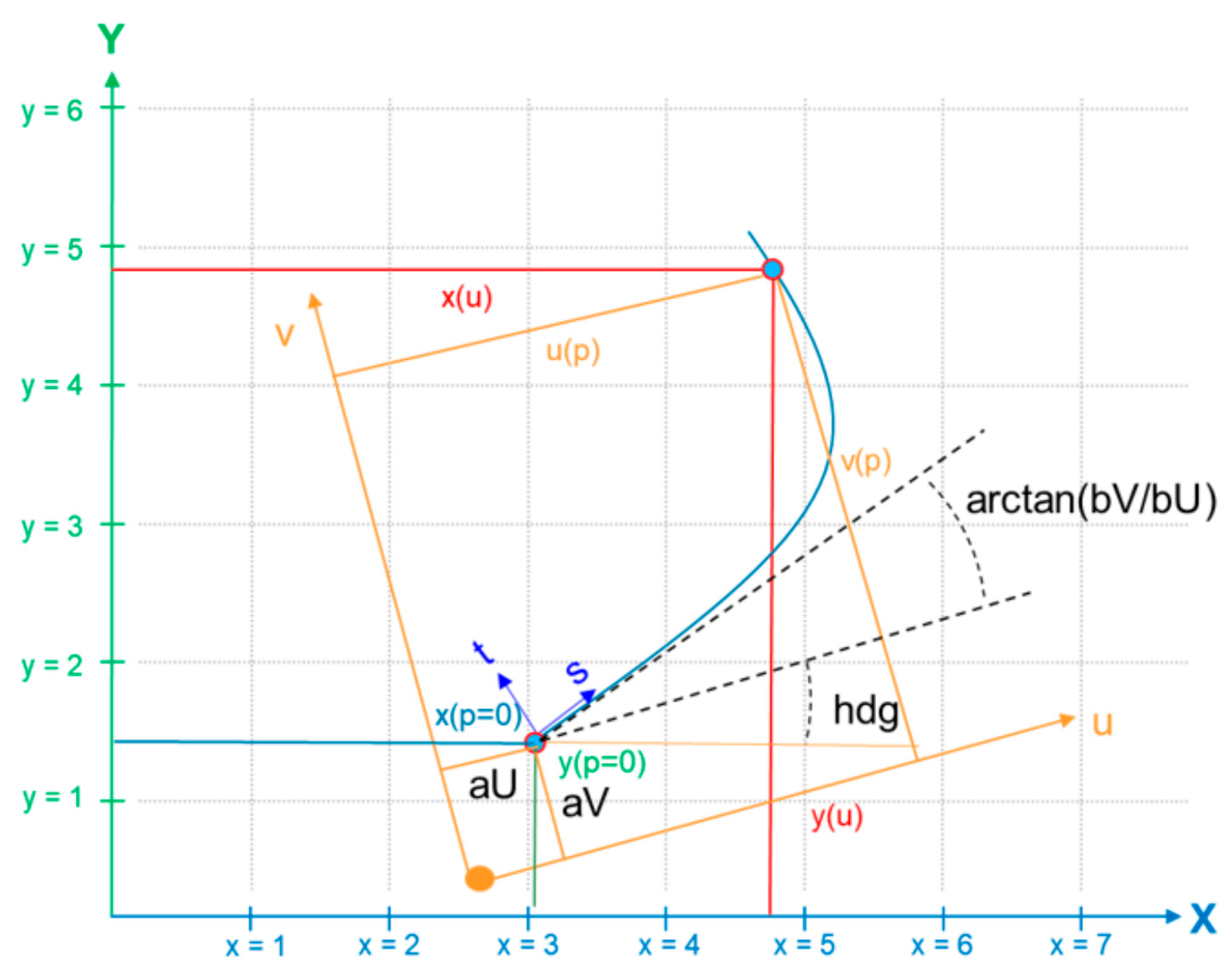
  For polynomials, parametric cubic curves are used to fit a part of a reference line. If no regulations are applied to curvatures, the related segment is defined as a polynomial. The structure of a polynomial in OpenDRIVE is presented as follows. The first step of generating roads in a polynomial is to convert related data from an inertial coordinate (x/y coordinate) to a local coordinate (u/v coordinate). The u coordinate is the axis along the start point of a reference line, and the v coordinate is the axis of lateral deviation from the first point of the reference line. According to the OpenDRIVE V1.6.1 User Guide published in 2021, to generate roads with parametric cubic curves, only x and y coordinates are required [8]. For consistency related to cubic polynomials, x and y coordinates may be calculated simultaneously as cubic polynomials by using local u and v coordinates, and cubic fitting may be applied to u and v coordinates with interpolation parameter p, which ranges from 0 to 1. The concept of a parametric cubic polynomial is expressed in Equations (5) and (6). and illustrated in Figure 6.

  u(p) = aU + bU × p + cU × p2 + dU × p3

  (5)

  v(p) = aV + bV × p + cV × p2 + dV × p3

  (6)

After the related geometric parameters were obtained, a parameter remained that had not been calculated: elevationProfile. In OpenDRIVE format, elevationProfile is presented as a cubic polynomial that fits all elevation values from the start point to the end point. A constant term is represented as “a”, and “d” represents a cubic term; this parameter is widely used in OpenDRIVE format if one parameter is presented as a cubic polynomial.

3.3.2. Length of Each Geometry

In OpenDRIVE, length is divided into three functions, and each geometry as a specific length function.

• Line:
  As previously indicated, the length of a line can be calculated using the Euclidean distance from the first point to the last point of a line. The relevant equation is as follows:

  $$Lengt{h}_L=\sqrt{{\left(x_n-x_1\right)}^2+{\left(y_n-y_1\right)}^2}$$

  (7)
• Arc:
  The circumference function is used for arc geometries, and the radius of an arc (R) is the reciprocal of its curvature. The relevant equation is presented as follows, where L is the Euclidean distance from the start point to the end point in an arc geometry.

  $$Lengt{h}_R=2\times \pi \times \frac{1}{curvature}\times \frac{si{n}^{-1}\left(\frac{\frac{L}{2}}{R}\right)\times 2}{{360}^{°}}$$

  (8)
• Polynomial and Spiral:
  No particular functions are used for polynomials and spirals; therefore, their lengths are calculated based on the sum of the distances within each interpolation.

3.3.3. Attributes in Lanes

In the lane part of OpenDRIVE, which is presented in this section, two major attributes determine lane information: lane ID, which determines whether the lane is to the left or right, and lane width. The first task is to correctly identify lane attributes in OpenDRIVE. The approach used is almost the same as that for the classification and modeling of polylines after extraction; this approach also requires the translation of x and y coordinates to s and t coordinates. After coordinate translation, the algorithm compares the t coordinate for the first point of each lane line and then provides the relative ID for each lane. The relative ID depends on the direction of the reference line. A rightmost lane is used as an example. If a road is a two-way road with two lanes for each direction, the ID of the rightmost lane with a t coordinate has a minimum value of −2; the ID for the leftmost lane with a t coordinate has a maximum value of 2. In OpenDRIVE, lane width is a cubic polynomial, and the expression is by cubic fitting the shortest distance of all points from reference lines to lane lines. Thus, some features related to lane width might be ignored; users must decide whether separating lanes into different sections is necessary.

4. Case Study

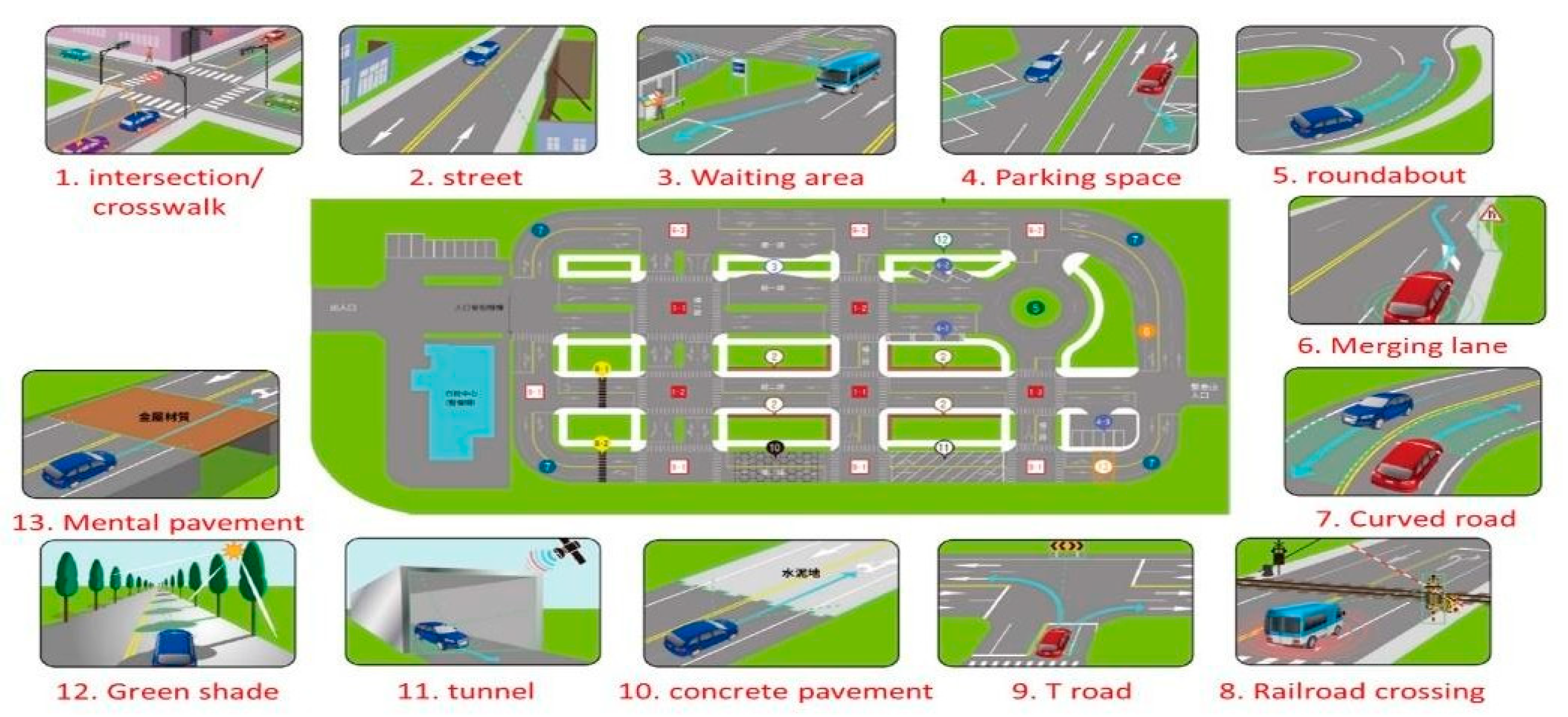
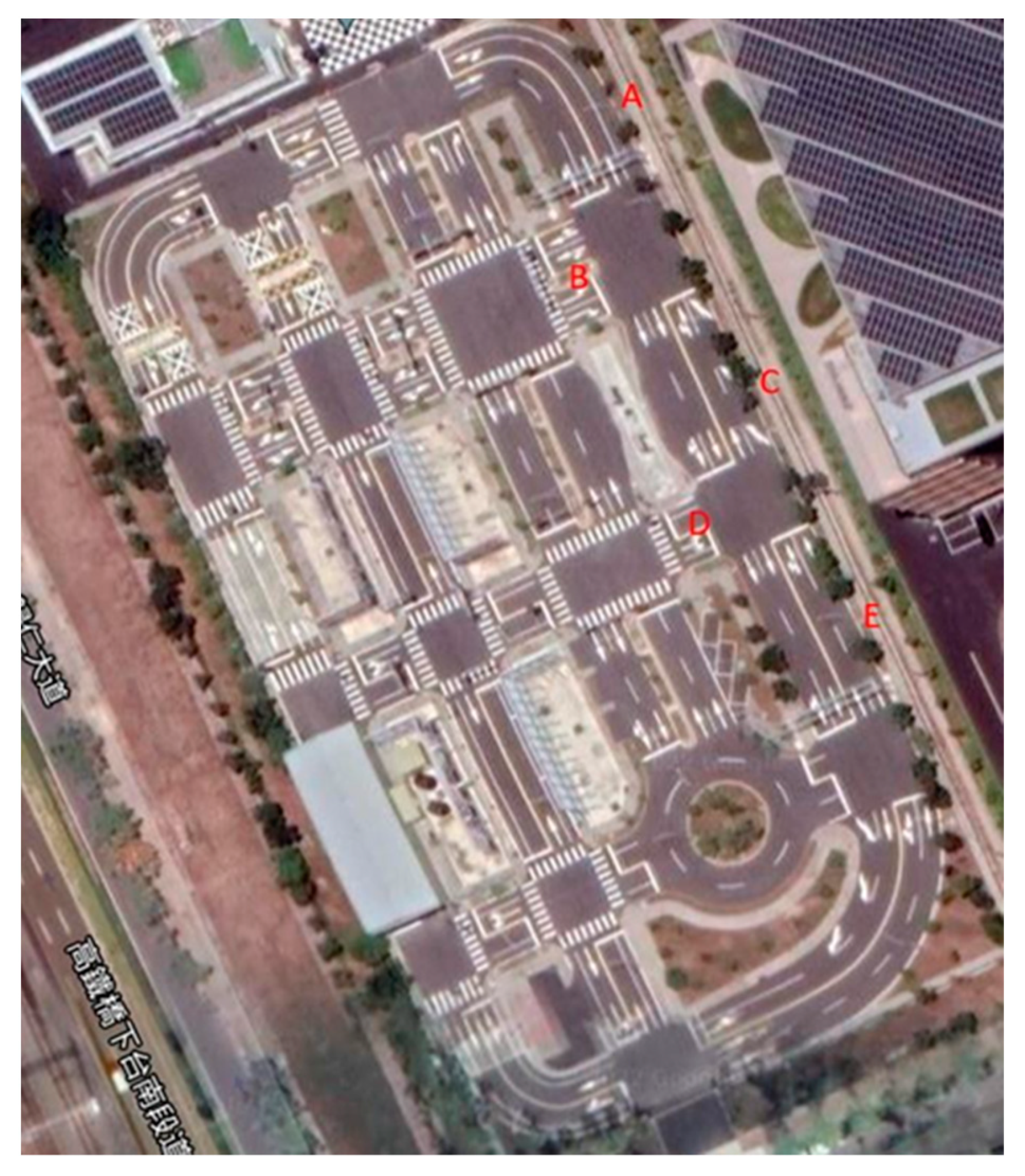
The experimental field in this study was the Taiwan CAR Lab, Tainan, Taiwan; this is an official test site for autonomous vehicles in Taiwan. It provides 13 traffic scenarios, as depicted in Figure 7. Five road segments (A, B, C, D, and E) were chosen to generate test data, as illustrated in Figure 8. Each segment has different characteristics, and the selection approach involved checking whether the proposed algorithm worked for various road types. Due to the test field limitations, some lane lines were missing; as such, related observations were lost in data extraction. The lost lane lines were the leftmost lane lines of A, C, and E and the top part of B; the results related to these sections are missing.

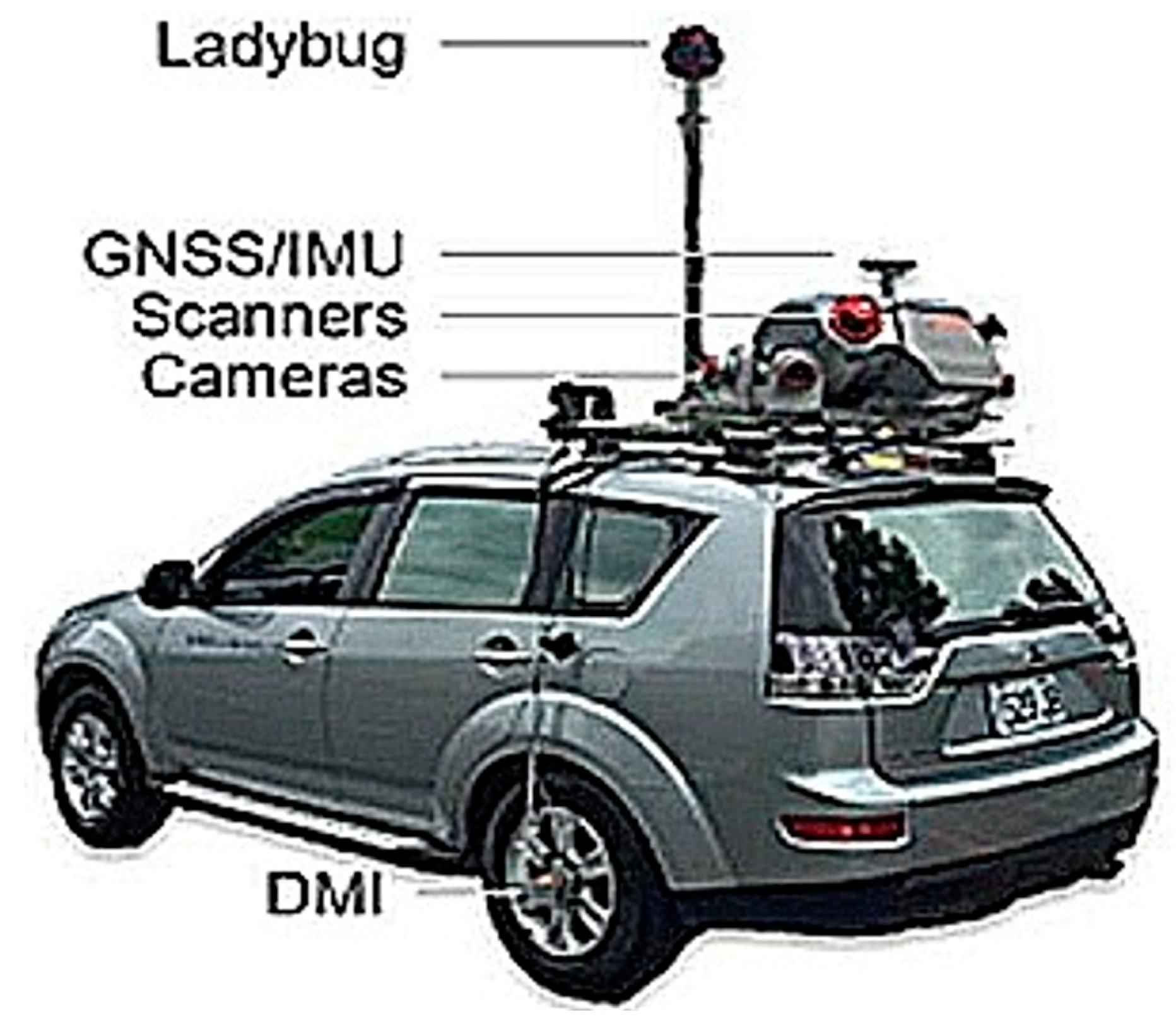
The sensors in the commercial mobile laser scanning (MLS) system contain a GNSS receiver, an IMU, cameras, laser scanners, a distance measurement instrument (DMI), and a ladybug. The specifications of the aforementioned sensors are presented in

Table 2. Specifications of sensors.

GNSS/IMU/DMI
Positioning (absolute)	20~50 (mm)
Positioning (relative)	10 (mm)
Scanners—VQ250
Laser pulse rate (PRR)	600 (kHz) (Max.)
Scan Rate	Up to 200 LPS
Accuracy	10 (mm)
Precision	5 (mm)
Cameras—CS6
Resolution	2452 × 2056
Pixel Size	3.45 × 3.45 (μm2)
Field of View	80° × 65° (H × V)
Exposure	38 (μs)~60 (s)

and Figure 9.

Since the previous trajectory provided by the mapping company deviates from true paths, some sections of the trajectory are on sidewalks. We observed these sections again using a higher-quality sensor. The specifications of this sensor (iMAR iNAV-RQH-10018) are presented in

Table 3. Specifications of iMAR iNAV-RQH-10018.

	Gyroscope	Accelerometer
Bias Instability	<0.002°/h	<10 μg
Random Walk Noise	<${0.0015}^{°}/\sqrt{\mathrm{h}}$	<$8 \mathsf{\mu }\mathrm{g}/\sqrt{\mathrm{Hz}}$

. An IMU and NovAtel PwrPak 7D-E2 were used as the GNSS receiver. iMAR iNAV-RQH-10018 is a navigation-grade INS, and its observational precision is sufficient for use in research contexts. We used NovAtel Inertial Explorer software to obtain new and reliable trajectory data.

The datasets in this case involve point cloud data and trajectories which passed through all lanes on five road segments as mentioned before in this experiment field. The quality of these datasets can be realized as above tables. The requirement of point cloud data is that the density of point cloud should be higher. Therefore, the authors pre-process the measurements from MLS system by point cloud registration. As for the trajectory data, it is required to pass through all lanes. When we need to classify the right-most lane line, it only needs trajectory data in one lane. When we need to define the center lane line, trajectories in all lanes are required. The definition the center lane line is that the directions of trajectories are different at both sides of lane line, and this lane line is defined as the center lane line.

5. Result and Discussion

The polylines modeled using the proposed algorithm were evaluated using an HD map of Taiwan that was produced by a mapping company and certified by an HD map research center in Taiwan. The comparison of the results and the reference data from the mapping company are shown in

Table 4. Polylines modeling results.

	2D	3D
Root Mean Square Error (RMSE)	0.045 (m)	0.062 (m)
Average Error	0.040 (m)	0.055 (m)
Standard Deviation (STD)	0.021 (m)	0.027 (m)

, and the comparison involved calculating the shortest distance from all points of the modeled polylines to all points in the reference data provided by the mapping company. The aforementioned company modeled lane lines manually from point cloud data before generating shapefiles and converting them to .csv files as reference data.

According to Taiwan HD map standards [15], the accuracy in 2D and 3D maps should be lower than 20 and 30 cm, respectively. All indicators in each dimension satisfied standard HD map requirements. The RMSE was used to estimate algorithm performance; the related measurements were 4.5 and 6.2 cm for the 2D and 3D maps, respectively.

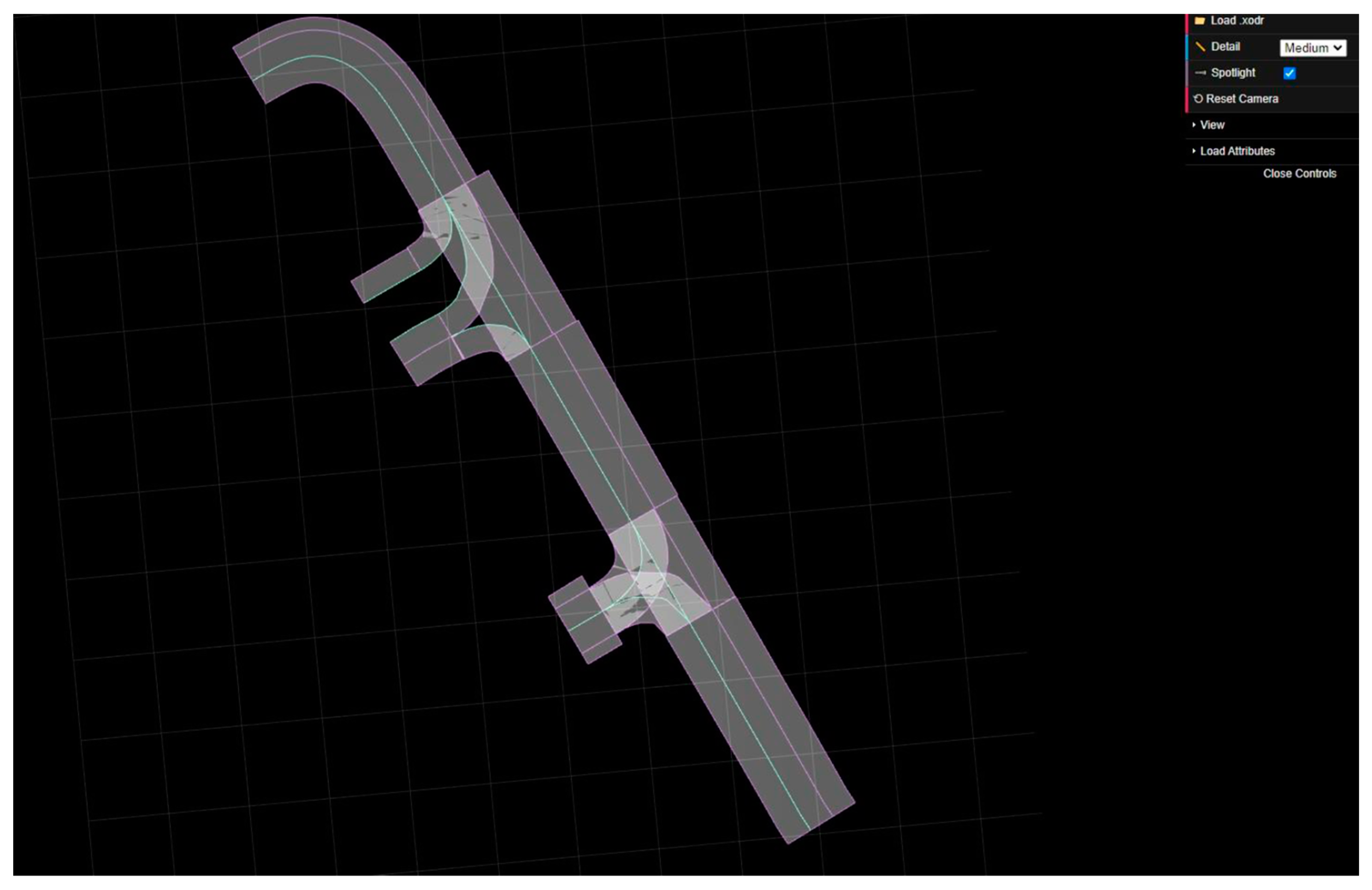
Figure 10 and Figure 11 represent the study result, made into OpenDRIVE, when it is imported into different platforms, such as OpenDRIVE Online Viewer, Google Earth, and the CAR Learning to Act (CARLA) simulator. Moreover, we could check whether the final OpenDRIVE file was available to be widely used. Figure 10 represents the study results in OpenDRIVE Online Viewer, a free online viewing tool for viewing HD maps. The tool allows people to directly open the files with the .xodr file extension and displays such files as a 3D model. The reference line (green) in Figure 10. was selected from one lane line. All roads were clearly visible in OpenDRIVE Online Viewer.

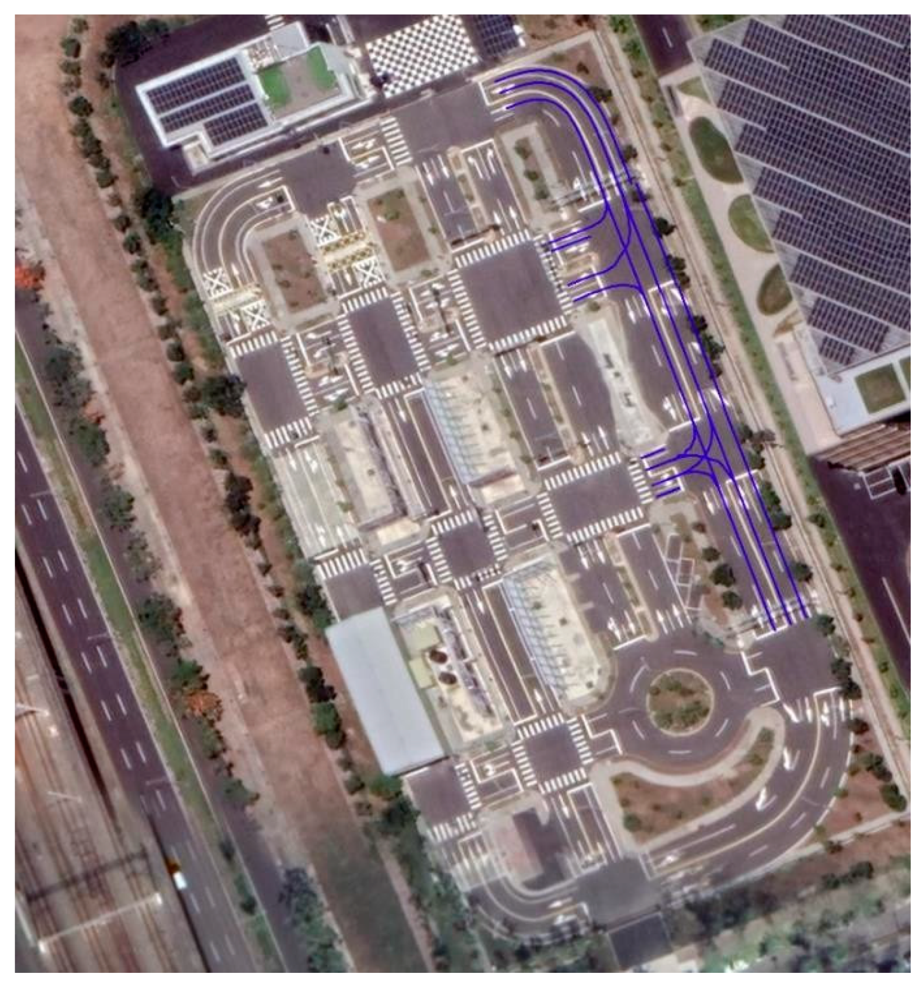
Figure 11 illustrates the converted elements in Google Earth, which only supports .kml files. To import the study results into Google Earth, the ASSURE Mapping tool was applied to transform the results in OpenDRIVE format to the Google Earth format. Since Google Earth map does not display lane width, the converted results retained only polylines that presented centerlines. After the conversion of the HD map, the centerline of each lane almost fit the satellite image.

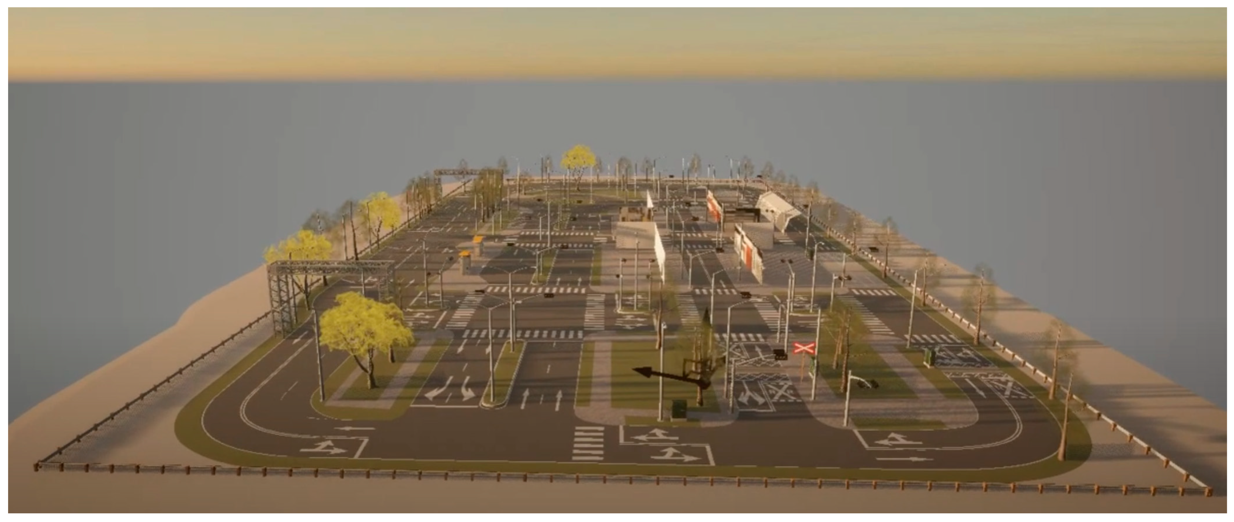
CARLA, a free and open-source simulator that allows people to import simulated scenes into it, supports simulations of OpenDRIVE files; furthermore, it can launch a driving scenario in these simulated scenes. Some researchers use this simulator for platform testing and for simulating the performance of algorithms for self-driving cars. The simulator provides some virtual meteorological conditions and vehicle models for situations. Figure 12 displays a simulation of the Taiwan CAR Lab environment; this environment was built using RoadRunner, a software program that enables the construction of virtual scenes and objects in OpenDRIVE files.

To compare the results after road modeling in OpenDRIVE format with reference data, the results must be converted into the vector map as a .csv file. The ASSURE Maps, which allowed conversion of HD maps, format was adopted to convert the HD maps from OpenDRIVE to the vector map. The relevant comparison is presented in

Table 5. Results achieved from modeling roads in OpenDRIVE format.

	2D	3D
Root Mean Square Error (RMSE)	0.069 (m)	0.079 (m)
Average Error	0.055 (m)	0.069 (m)
Standard Deviation (STD)	0.042 (m)	0.039 (m)

.

As indicated in Table 5, all the indicators fulfill the accuracy requirements of Taiwan HD map standards; the accuracy in 2D was better than that in 3D. The errors from modeling polylines and roads in OpenDRIVE format can be explained by the inaccuracy of the method for obtaining mean curvatures and the fact that geometric parameters cannot represent roads without error. Furthermore, the results were compared after maps were translated from shapefiles provided by the mapping company, and some distortion was inevitable during this step. However, the results are still reliable; the RMSE was 6.9 and 7.9 cm for 2D and 3D maps, respectively. Moreover, time consumption in each phase is shown in

Table 6. Time consumption of each phase of OpenDRIVE generation.

	Automated Generation	Traditional Generation
Lane Line Point Cloud Extraction	About 5 min
Modelling Lane Line	About 15 s
OpenDRIVE Generation	About 41 s
Total	About 6 min	Days~months

, and the methodology proposed in this study reduce huge time of production. This is a dependable result indicating that automatically modeled roads in OpenDRIVE format meet the HD maps standard.

6. Conclusions

HD maps are important for supporting AV journeys and improving navigation. However, the costs associated with the manual production of HD maps are substantial. Furthermore, no automatic map generation approach has been extensively applied. In this study, an algorithm was proposed that can automatically generate HD maps for roads with multiple lanes in OpenDRIVE format. The algorithm involves road element extraction and lane line modeling. In the extraction part, CSF and region growing–based road edge extraction are applied to obtain road markings in high-intensity data sets, as classified using an intensity filter. During modeling, the algorithm first classifies the extraction data set into different lane lines and then models them together through cubic spline fitting. Subsequently, it extracts geometric parameters in OpenDRIVE format to construct an HD map. Furthermore, the algorithm’s results satisfy reliability standards related to HD maps in Taiwan. The accuracy level was 6.9 and 7.9 cm for 2D and 3D maps, respectively. The algorithm reduces the time spent on HD map production. Moreover, the ASSURE tool can be used to transform the algorithm results to other HD map formats [7].