
Mapping Urban and Peri-Urban Land Cover in Zimbabwe: Challenges and Opportunities

Abstract
:1. Introduction
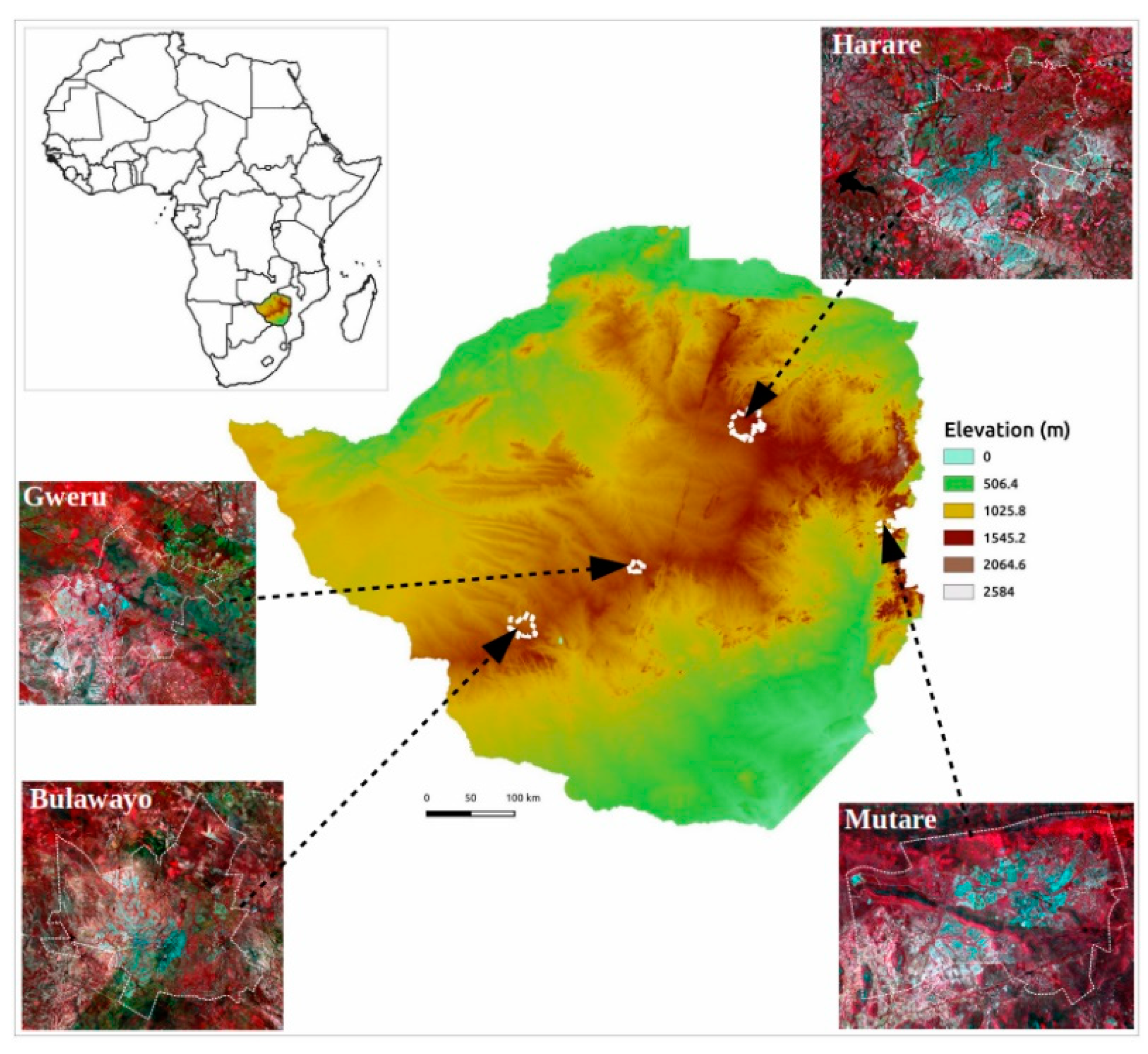
2. Study Area
3. Methods
3.1. Data Preparation
3.1.1. Satellite Imagery
3.1.2. Reference Data for Land Cover Classification
3.1.3. Land Cover Mapping Approach
4. Results
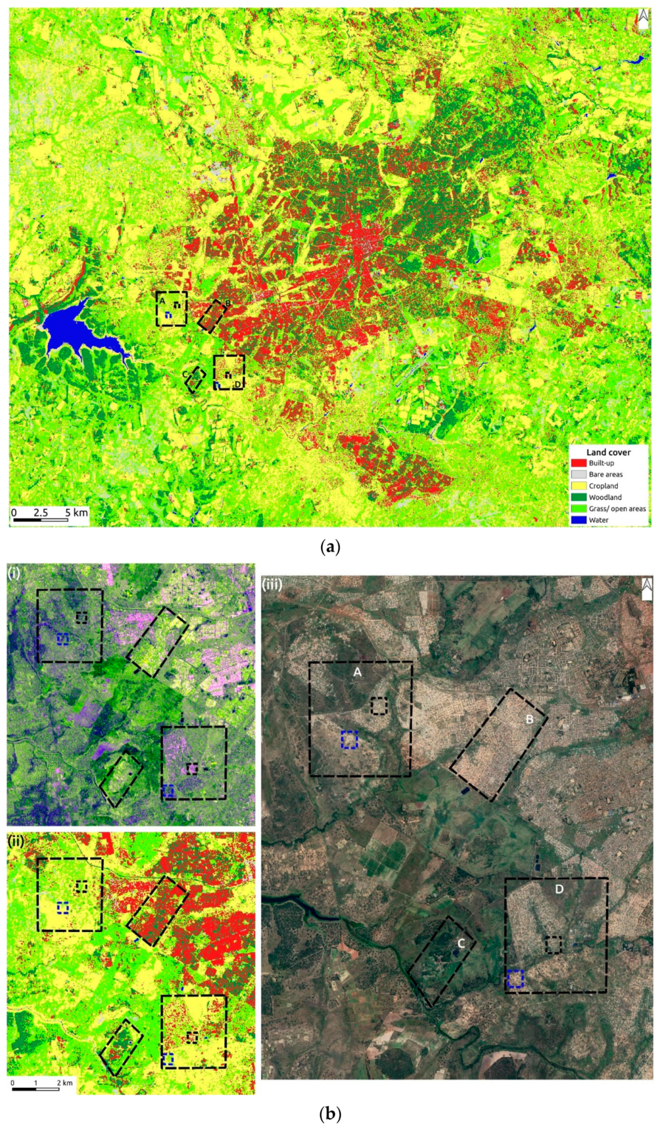
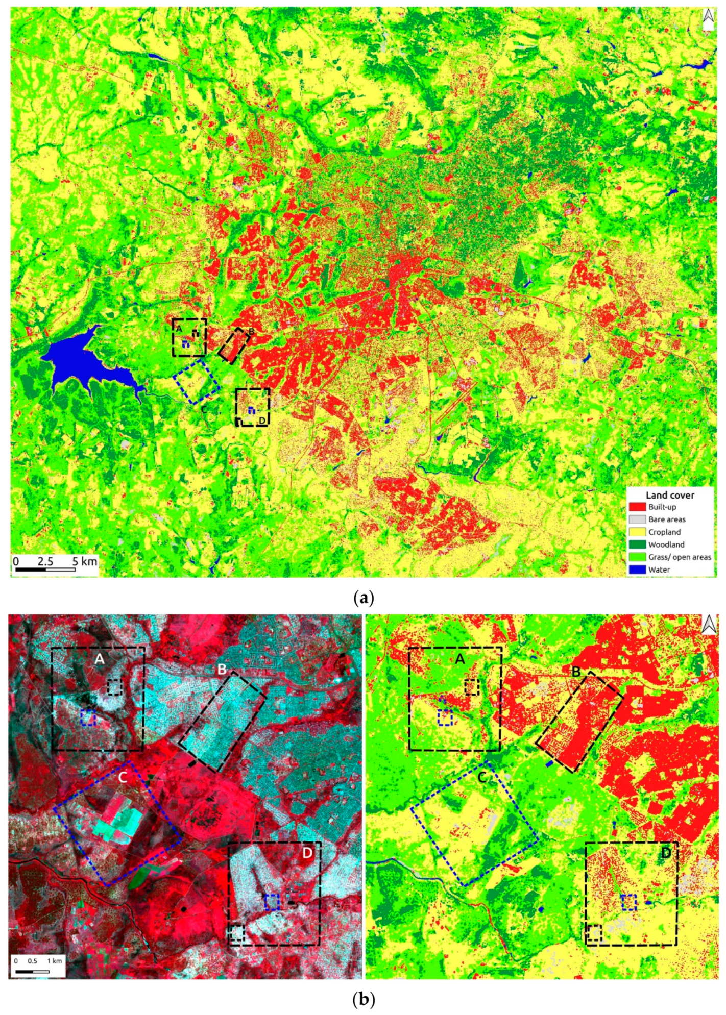
4.1. Land Cover Mapping and Analysis for Harare
4.1.1. Evaluation of the Training and Test Models
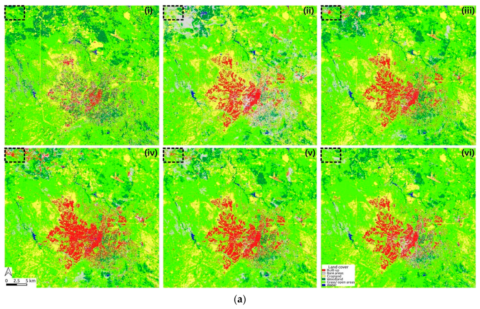
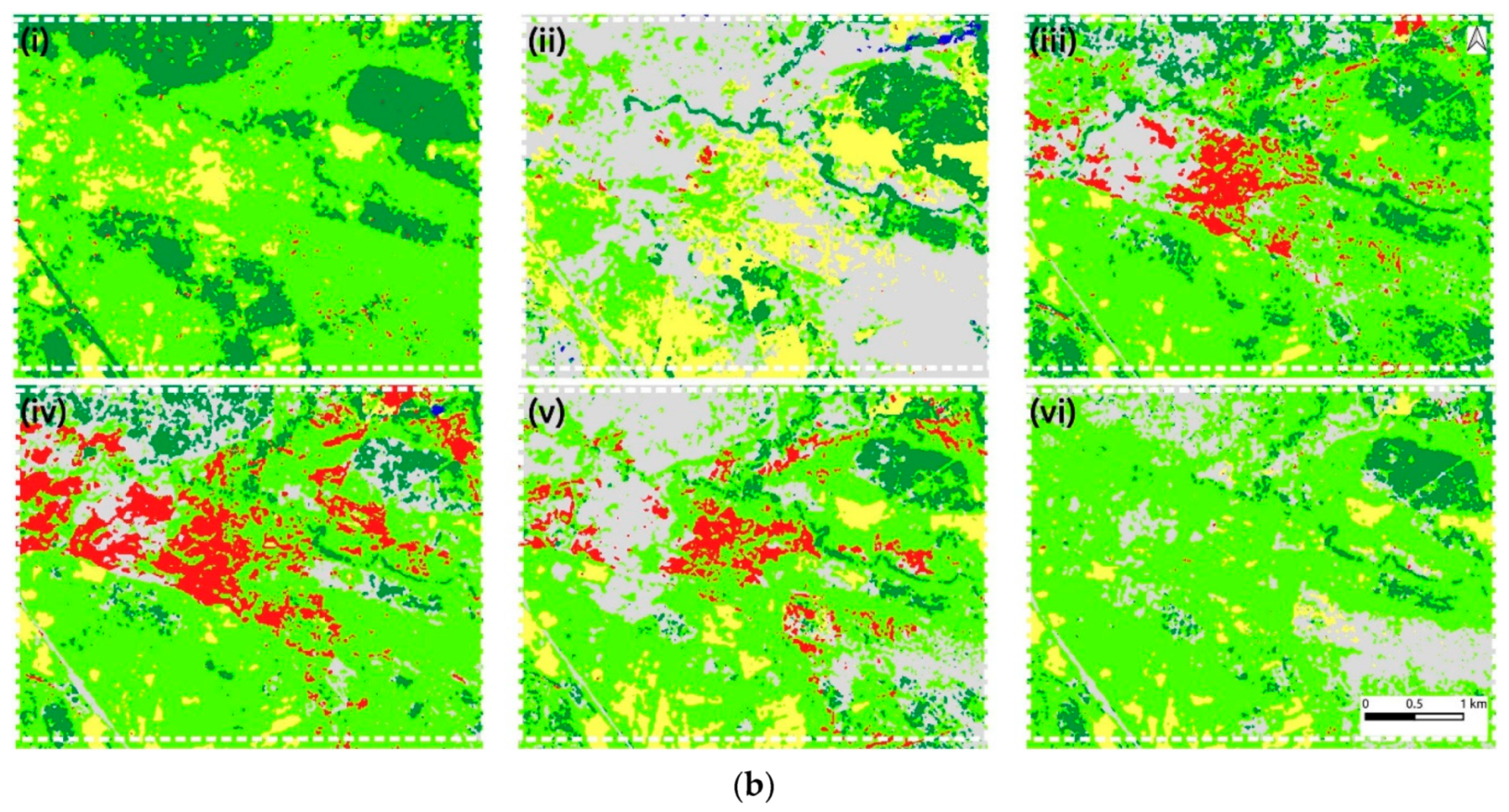
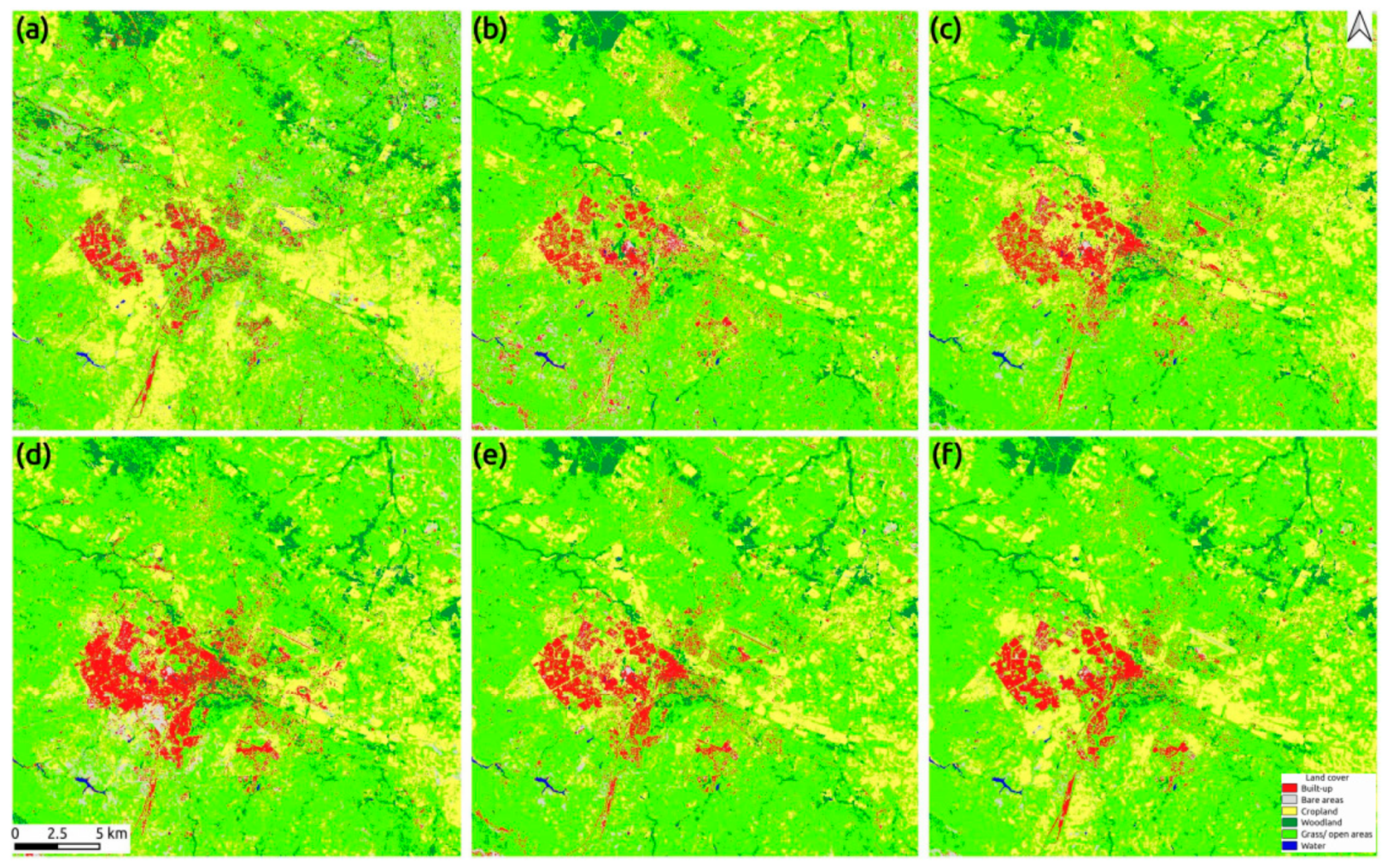
4.1.2. Evaluation of Land Cover Maps
4.1.3. Classification Accuracy Assessment
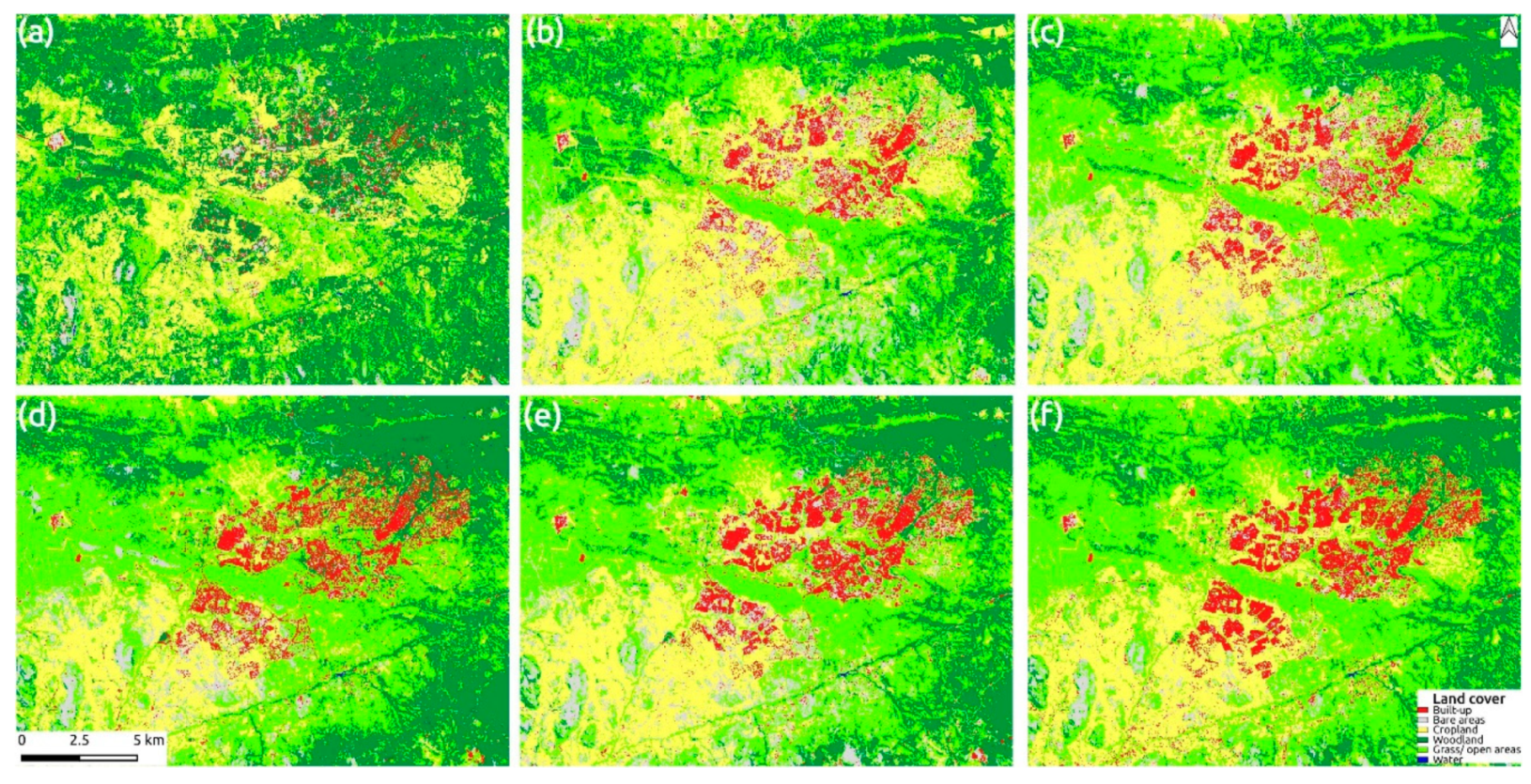
4.2. Land Cover Mapping in Other Major Urban Centers in Zimbabwe
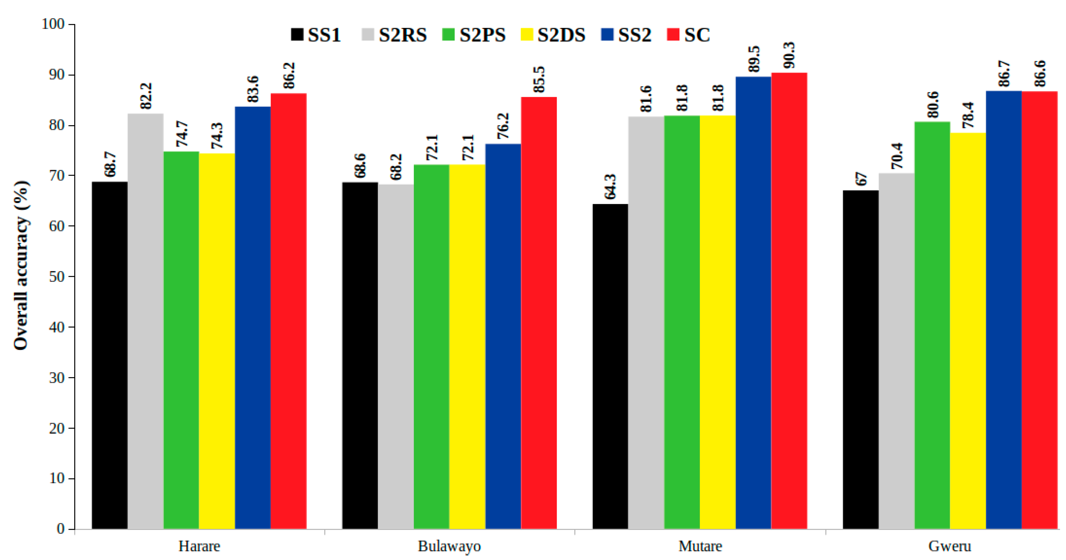
4.2.1. Comparison of Model Overall Accuracy
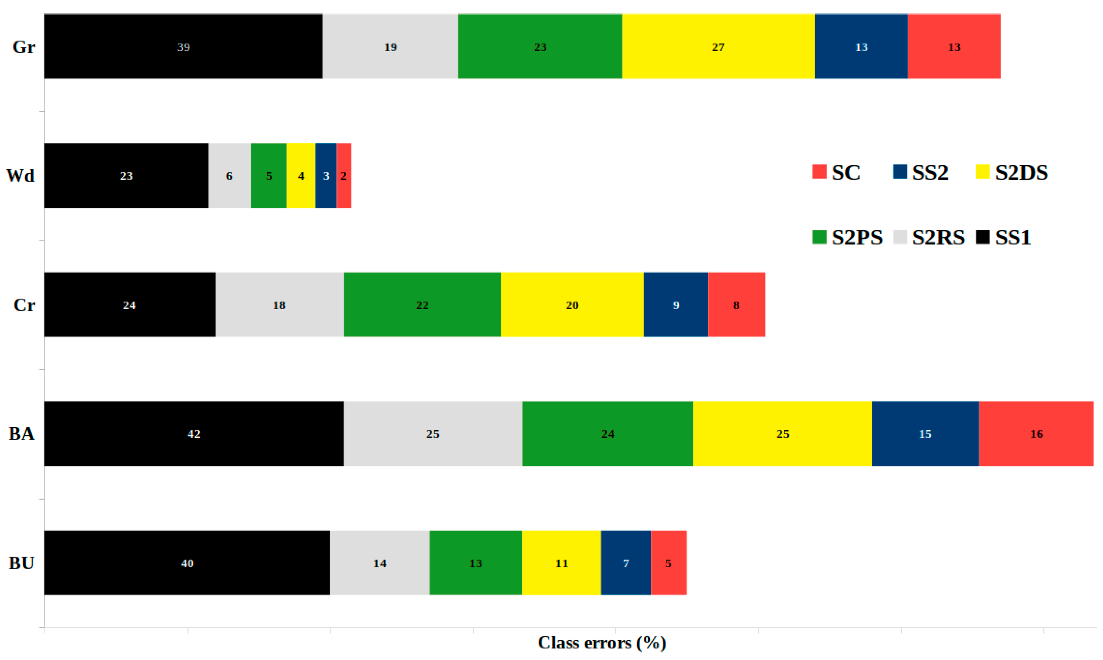
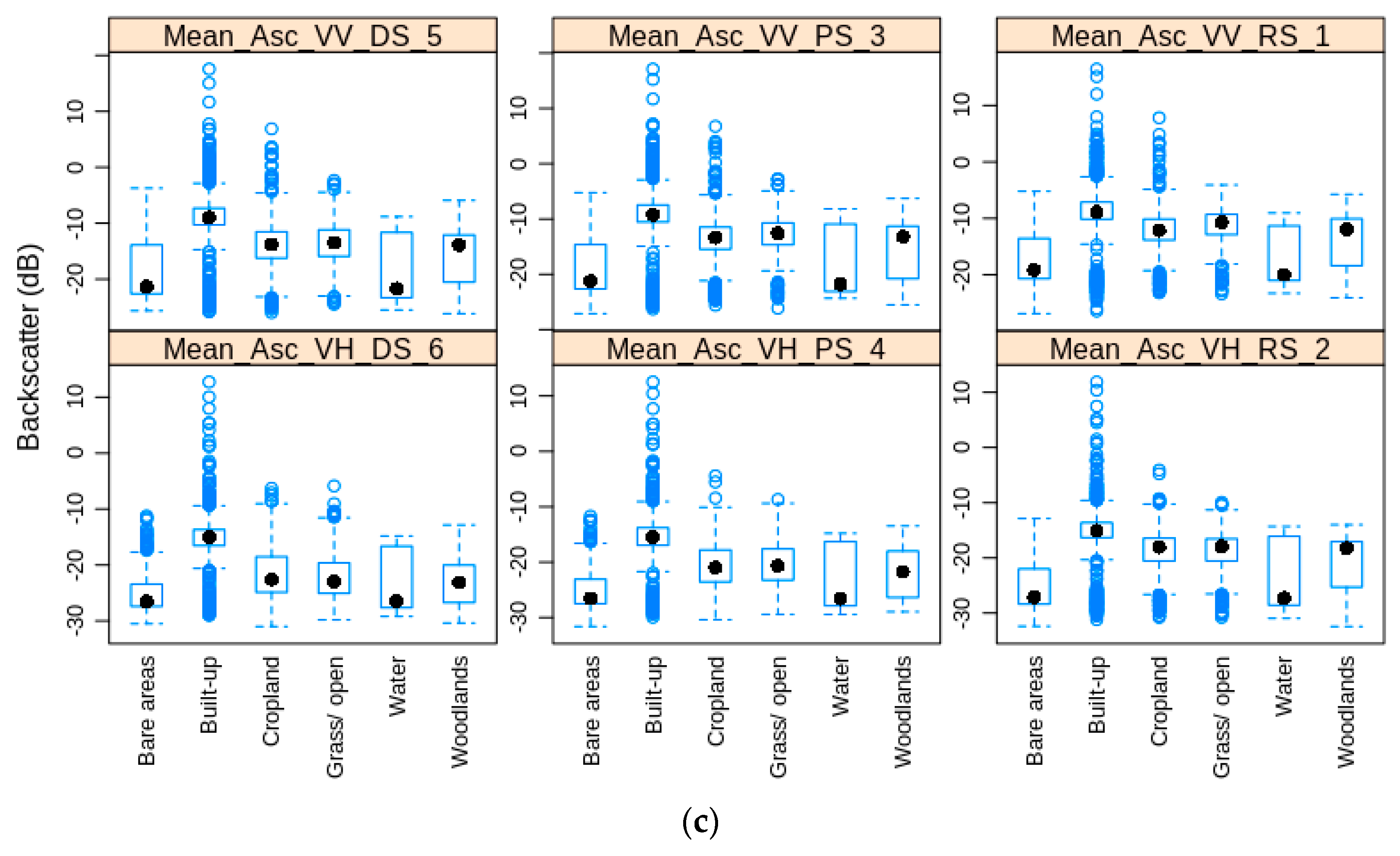
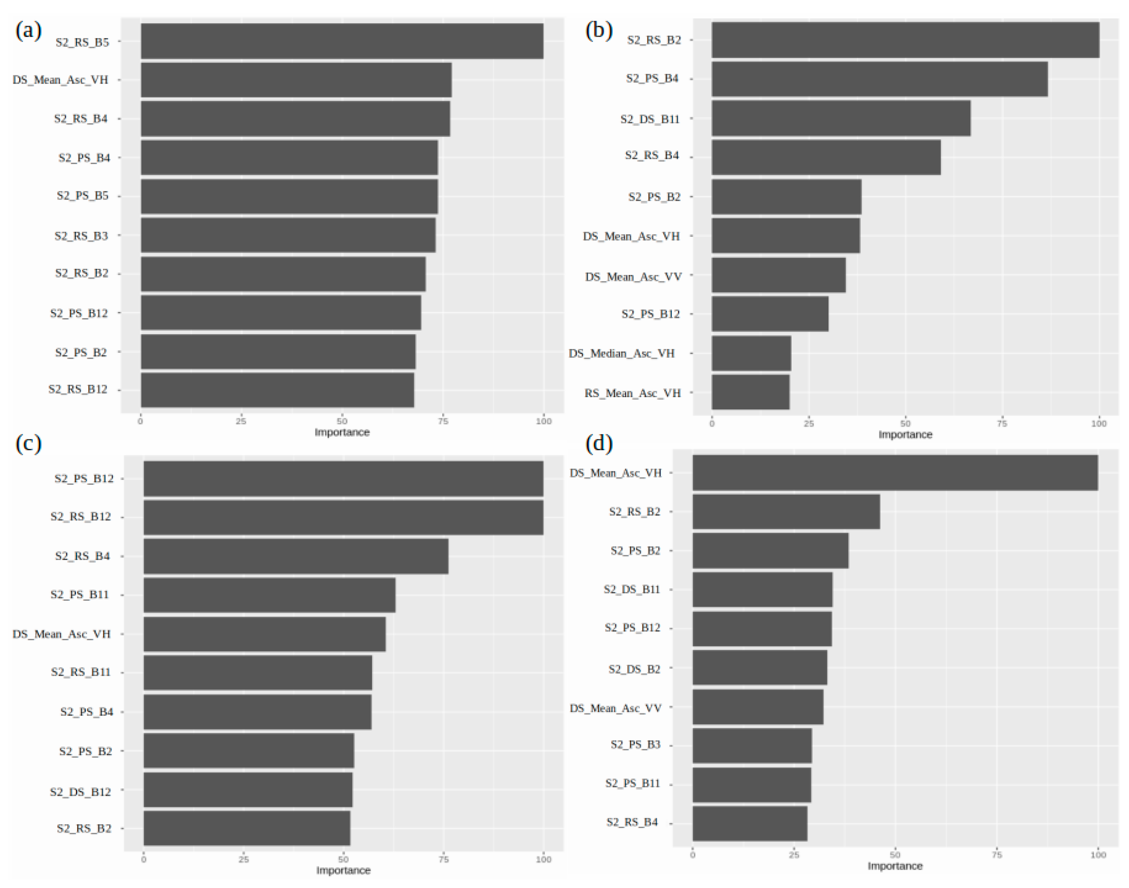
4.2.2. Random Forest Feature Importance
5. Discussion
6. Conclusions
Supplementary Materials
Author Contributions
Funding
Institutional Review Board Statement
Informed Consent Statement
Data Availability Statement
Conflicts of Interest
References
- UNHabitat. The Strategic Plan 2020–2023. Available online: https://unhabitat.org/sites/default/files/documents/2019-09/strategic_plan_2020-2023.pdf (accessed on 1 September 2020).
- World Health Organization. Urban Population Growth. 2020. Available online: https://www.who.int/gho/urban_health/situation_trends/urban_population_growth_text/en/ (accessed on 31 August 2020).
- Maktav, D.; Erbek, F.S. Analysis of urban growth using multi-temporal satellite data in Istanbul, Turkey. Int. J. Remote Sens. 2005, 26, 797–810. [Google Scholar] [CrossRef]
- Bello-Schuneman, J. Defining the future of Africa’s brave new world. Afr. Fact. 2018, 45, 12–18. [Google Scholar]
- Seto, K.C.; Fragkias, M.; Güneralp, B.; Reilly, M.K. A Meta-Analysis of Global Urban Land Expansion. PLoS ONE 2011, 6, e23777. [Google Scholar] [CrossRef]
- Schneider, A. Monitoring land cover change in urban and peri-urban areas using dense time stacks of Landsat satellite data and a data mining approach. Remote Sens. Environ. 2012, 124, 689–704. [Google Scholar] [CrossRef]
- United Nations. 68% of the World Population Projected to Live in Urban Areas by 2050, Says UN. 2018. Available online: https://www.un.org/development/desa/en/news/population/2018-revision-of-world-urbanization-prospects.html (accessed on 31 August 2020).
- Zerbo, A.; Delgado, R.C.; González, P.A. Vulnerability and everyday health risks of urban informal settlements in Sub-Saharan Africa. Glob. Health J. 2020, 4, 46–50. [Google Scholar] [CrossRef]
- United Nations. World Urbanization Prospects 2018: Highlights; Department of Economic and Social Affairs Population Division: New York, NY, USA, 2019. [Google Scholar]
- Schug, F.; Okujeni, A.; Hauer, J.; Hostert, P.; Nielsen, J.Ø.; van der Linden, S. Mapping patterns of urban development in Ouagadougou, Burkina Faso, using machine learning regression modeling with bi-seasonal Landsat time series. Remote Sens. Environ. 2018, 210, 217–228. [Google Scholar] [CrossRef]
- Conitz, M.W. GIS applications in Africa: Introduction. Photogram Eng. Remote Sens. 2000, 66, 672–673. [Google Scholar]
- UN-HABITAT. The State of African Cities 2008—A Framework for Addressing Urban Challenges in Africa; UN-HABITAT: Nairobi, Kenya, 2008. [Google Scholar]
- Wania, A.; Kemper, T.; Tiede, D.; Zeil, P. Mapping recent built-up area changes in the city of Harare with high resolution satellite imagery. Appl. Geogr. 2014, 46, 35–44. [Google Scholar] [CrossRef]
- Lu, D.; Weng, Q. A survey of image classification methods and techniques for improving classification performance. Int. J. Remote Sens. 2007, 28, 823–870. [Google Scholar] [CrossRef]
- Nemmour, H.; Chibani, Y. Multiple support vector machines for land cover change detection: An application for mapping urban extensions. ISPRS J. Photogramm. Remote Sens. 2006, 61, 125–133. [Google Scholar] [CrossRef]
- Pal, M.; Mather, P.M. Support vector machines for classification in remote sensing. Int. J. Remote Sens. 2005, 26, 1007–1011. [Google Scholar] [CrossRef]
- Rodriguez-Galiano, V.F.; Chica-Olmo, M.; Abarca-Hernandez, F.; Atkinson, P.M.; Jeganathan, C. Random Forest classifica-tion of Mediterranean land cover using multi-seasonal imagery and multi-seasonal texture. Remote Sens. Environ. 2012, 121, 93–107. [Google Scholar] [CrossRef]
- Ma, L.; Liu, Y.; Zhang, X.; Ye, Y.; Yin, G.; Johnson, B.A. Deep learning in remote sensing applications: A meta-analysis and review. ISPRS J. Photogramm. Remote Sens. 2019, 152, 166–177. [Google Scholar] [CrossRef]
- Griffiths, P.; Hostert, P.; Gruebner, O.; van der Linden, S. Mapping megacity growth with multi-sensor data. Remote Sens. Environ. 2010, 114, 426–439. [Google Scholar] [CrossRef]
- Zhu, Z.; Zhou, Y.; Seto, K.C.; Stokes, E.C.; Deng, C.; Pickett, T.A.; Taubenböck, H. Understanding an urbanizing planet: Stra-tegic directions for remote sensing. Remote Sens. Environ. 2019, 228, 164–182. [Google Scholar] [CrossRef]
- Güneralp, B.; Lwasa, S.; Masundire, H.; Parnell, S.; Seto, K.C. Urbanization in Africa: Challenges and opportunities for conservation. Environ. Res. Lett. 2017, 13, 015002. [Google Scholar] [CrossRef]
- Mundia, C.N.; Aniya, M. Analysis of land use/cover changes and urban expansion of Nairobi city using remote sensing and GIS. Int. J. Remote Sens. 2005, 26, 2831–2849. [Google Scholar] [CrossRef]
- Gamanya, R.; de Maeyer, P.; de Dapper, M. Object-oriented change detection for the city of Harare, Zimbabwe. Expert Syst. Appl. 2009, 36, 571–588. [Google Scholar] [CrossRef]
- Forkuor, G.; Cofie, O. Dynamics of land-use and land-cover change in Freetown, Sierra Leone and its effects on urban and peri-urban agriculture—A remote sensing approach. Int. J. Remote Sen. 2011, 32, 1017–1037. [Google Scholar] [CrossRef]
- Kamusoko, C.; Gamba, J.; Murakami, H. Monitoring Urban Spatial Growth in Harare Metropolitan Province, Zimbabwe. Adv. Remote Sens. 2013, 2, 322–331. [Google Scholar] [CrossRef] [Green Version]
- Vermeiren, K.; van Rompaey, A.; Loopmans, M.; Serwajja, E.; Mukwaya, P.I. Urban growth of Kampala, Uganda: Pattern analysis and scenario development. Landsc. Urban. Plan. 2012, 106, 199–206. [Google Scholar] [CrossRef]
- Simwanda, M.; Murayama, Y. Integrating Geospatial Techniques for Urban Land Use Classification in the Developing Sub-Saharan African City of Lusaka, Zambia. ISPRS Int. J. Geo-Inf. 2017, 6, 102. [Google Scholar] [CrossRef] [Green Version]
- Korah, P.I.; Matthews, T.; Tomerini, D. Characterising spatial and temporal patterns of urban evolution in Sub-Saharan Africa: The case of Accra, Ghana. Land Use Policy 2019, 87. [Google Scholar] [CrossRef]
- Magidi, J.; Ahmed, F. Assessing urban sprawl using remote sensing and landscape metrics: A case study of City of Tshwane, South Africa (1984–2015). Egypt. J. Remote Sens. Space Sci. 2019, 22, 335–346. [Google Scholar] [CrossRef]
- Mohamed, A.; Worku, H. Quantification of the land use/land cover dynamics and the degree of urban growth goodness for sustainable urban land use planning in Addis Ababa and the surrounding Oromia special zone. J. Urban. Manag. 2019, 8, 145–158. [Google Scholar] [CrossRef]
- Goldblatt, R.; Deininger, K.; Hanson, G. Utilizing publicly available satellite data for urban research: Mapping built-up land cover and land use in Ho Chi Minh City, Vietnam. Dev. Eng. 2018, 3, 83–99. [Google Scholar] [CrossRef]
- Knorn, J.; Rabe, A.; Radeloff, V.C.; Kuemmerle, T.; Kozak, J.; Hostert, P. Land cover mapping of large areas using chain clas-sification of neighboring Landsat satellite images. Remote Sens. Environ. 2009, 113, 957–964. [Google Scholar] [CrossRef]
- Jensen, J.R. Remote Sensing of the Environment: An Earth Resource Perspective. Pearson Educ. 2000, 407–470. [Google Scholar]
- Schug, F.; Frantz, D.; Okujeni, A.; van der Linden, S.; Hostert, P. Mapping urban-rural gradients of settlements and vegeta-tion at national scale using Sentinel-2 spectral-temporal metrics and regression-based unmixing with synthetic training data. Remote Sens. Environ. 2020, 246, 111810. [Google Scholar] [CrossRef]
- Forkuor, G.; Dimobe, K.; Serme, I.; Tondoh, J.E. Landsat-8 vs. Sentinel-2: Examining the added value of sentinel-2’s red-edge bands to land-use and land-cover mapping in Burkina Faso. GIScience Remote Sens. 2018, 55, 331–354. [Google Scholar] [CrossRef]
- Pesaresi, M.; Corbane, C.; Julea, A.; Florczyk, A.J.; Syrris, V.; Soille, P. Assessment of the Added-Value of Sentinel-2 for Detecting Built-up Areas. Remote Sens. 2016, 8, 299. [Google Scholar] [CrossRef] [Green Version]
- Kamusoko, C.; Gamba, J. Simulating Urban Growth Using a Random Forest-Cellular Automata (RF-CA) Model. ISPRS Int. J. Geo-Inf. 2015, 4, 447–470. [Google Scholar] [CrossRef]
- Zimbabwe National Statistics Agency (ZimStats). Census 2012: Preliminary Report; Zimbabwe National Statistics Agency: Harare, Zimbabwe, 2012. [Google Scholar]
- Mbiba, B. On the Periphery: Missing Urbanisation in Zimbabwe. 2017. Available online: https://www.africaresearchinstitute.org/newsite/publications/periphery-missing-urbanisation-zimbabwe/ (accessed on 1 September 2020).
- Infrastructure and Cities for Economic Development. Zimbabwe’s Changing Urban Landscape: Evidence and Insights on Zim-babwe’s Urban Trends. 2017. Available online: https://assets.publishing.service.gov.uk/media/59521681e5274a0a5900004a/ICED_Evidence_Brief_-_Zimbabwe_Urban_Trends_-_Final.pdf (accessed on 19 October 2020).
- Patel, D. Some issues of urbanisation and development in Zimbabwe. J. Soc. Dev. Afr. 1998, 3, 17–31. [Google Scholar]
- Gorelick, N.; Hancher, M.; Dixon, M.; Ilyushchenko, S.; Thau, D.; Moore, R. Google Earth Engine: Planetary-scale geospatial analysis for everyone. Remote Sens. Environ. 2017, 202, 18–27. [Google Scholar] [CrossRef]
- Yuan, F.; Sawaya, K.E.; Loeffelholz, B.C.; Bauer, M.E. Land cover classification and change analysis of the Twin Cities (Min-nesota) Metropolitan area by multitemporal Landsat remote sensing. Remote Sens. Environ. 2005, 98, 317–328. [Google Scholar] [CrossRef]
- ESA. Sentinel-2 User Handbook. 2015. Available online: https://doi.org/10.13128/REA-22658 (accessed on 1 August 2020).
- European Space Agency (ESA). SAR Formats. 2020. Available online: https://earth.esa.int/web/sentinel/technical-guides/sentinel-1-sar/products-algorithms/level-1-product-formatting (accessed on 19 October 2020).
- Eckardt, R.; Urbazaev, M.; Salepci, N.; Pathe, C.; Schmullius, C.; Woodhouse, I.; Stewart, C. Echoes in Space: Introduction to Radar Remote Sensing; European Space Agency and EO College: Frascati, Italy, 2019. [Google Scholar]
- Leutner, B.; Horning, N.; Schwalb-Willmann, J.; Hijmans, R.J. Package Rstoolbox. 2019. Available online: https://cran.r-project.org/web/packages/RStoolbox/RStoolbox.pdf (accessed on 20 July 2020).
- R Development Core Team. R: A Language and Environment for Statistical Computing. R Foundation for Statistical Compu-ting. 2005. Available online: http://r-pro-ject.kr/sites/default/files/2%EA%B0%95%EA%B0%95%EC%A2%8C%EC%86%8C%EA%B0%9C_%EC%8B%A0%EC%A2%85%ED%99%94.pdf (accessed on 3 April 2014).
- Breiman, L. Random forests. Mach. Learn. 2001, 45, 5–32. [Google Scholar] [CrossRef] [Green Version]
- Mellor, A.; Haywood, A.; Stone, C.; Jones, S. The performance of random forests in an operational setting for large area scle-rophyll forest classification. Remote Sens. 2013, 5, 2838–2856. [Google Scholar] [CrossRef] [Green Version]
- Walton, J.T. Subpixel urban land cover estimation: Comparing cubist, random forests, and support vector regression. Photogramm. Eng. Remote Sens. 2008, 74, 1213–1222. [Google Scholar] [CrossRef] [Green Version]
- Kuhn, M.; Johnson, K. Applied Predictive Modeling; Springer: Berlin, Germany, 2016. [Google Scholar]
- Mather, P.M.; Koch, M. Computer Processing of Remotely-Sensed Images: An Introduction; Wiley-Blackwell: Hoboken, NJ, USA, 2011. [Google Scholar]
- Ainsworth, T.L.; Schuler, D.L.; Lee, J.S. Polarimetric SAR characterization of man-made structures in urban areas using nor-malized circular-pol correlation coefficients. Remote Sens. Environ. 2008, 112, 2876–2885. [Google Scholar] [CrossRef]
- Bryan, M.L. The effect of radar azimuth angle on cultural data. Photogram. Eng. Remote Sens. 1979, 45, 1097–1107. [Google Scholar]
- Hardaway, G.; Gustafs, G.C.; Lichy, D. Cardinal effect on Seasat images of urban areas. Photogram Eng. Remote Sens. 1982, 48, 399–404. [Google Scholar]
- Sabins, F.F. Remote Sensing: Principles and Interpretation; W. H. Freeman and Company: New York, NY, USA, 1997; pp. 177–240. [Google Scholar]
- Olofsson, P.; Foody, G.M.; Stehman, S.V.; Woodcock, C.E. Making better use of accuracy data in land change studies: Esti-mating accuracy and area and quantifying uncertainty using stratified estimation. Remote Sens. Environ. 2013, 129, 122–131. [Google Scholar] [CrossRef]
- Olofsson, P.; Herold, M.; Stehman, S.V.; Woodcock, C.E.; Wulder, M.A. Good practices for estimating area and assessing ac-curacy of land change. Remote Sens. Environ. 2014, 148, 42–57. [Google Scholar] [CrossRef]
- Cochran, W.G. Sampling Techniques; John Wiley & Sons: New York, NY, USA, 1977. [Google Scholar]
- Zhu, Z.; Woodcock, C.E.; Rogan, J.; Kellndorfer, J. Assessment of spectral, polarimetric, temporal, and spatial dimensions for urban and peri-urban land cover classification using Landsat and SAR data. Remote Sens. Environ. 2012, 117, 72–82. [Google Scholar] [CrossRef]
- Abdikan, S.; Sanli, F.B.; Ustuner, M.; Calò, F. Land cover mapping using Sentinel-1 SAR data. Int. Arch. Photogram. Remote Sens. Spat. Inf. Sci. 2016, 41, 757–761. [Google Scholar] [CrossRef]
- Dong, Y.; Forster, B.; Ticehurst, C. Radar backscatter analysis for urban environments. Int. J. Remote Sens. 1997, 18, 1351–1364. [Google Scholar] [CrossRef]
- Niu, X. Multitemporal Spaceborne Polarimetric SAR data for Urban Land Cover Mapping. Ph.D. Thesis, KTH Royal Institute of Technology, Stockholm, Sweden, 2012. [Google Scholar]
- Li, X.; Zhou, Y.; Gong, P.; Seto, K.C.; Clinton, N. Developing a method to estimate building height from Sentinel-1 data. Remote Sens. Environ. 2020, 240, 111705. [Google Scholar] [CrossRef]
- Molch, K. Radar Earth Observation Imagery for Urban Area Characterisation. JRC Sci. Tech. Rep. 2009, 1–9. [Google Scholar] [CrossRef]


| Compiled Imagery | Date Range | Season | Number of Images/Bands | Remarks |
|---|---|---|---|---|
| Mean and median S1 | 1 January–30 March 2020 | Rainy | 4 | IW swath mode 250 km, VV and VH polarization, pixel spacing 10 m, Ascending orbit |
| 1 April–30 June 2020 | Post-rainy | 4 | ||
| 1 July–30 October 2020 | Dry | 4 | ||
| Median S2 | 1 January–30 March 2020 | Rainy | 9 | Bands 2, 3, 4, 8, at 10 m spatial resolution; Bands 5, 6, 7, 8a, 11, and 12 resampled to 10 m |
| 1 April–30 June 2020 | Post-rainy | 9 | ||
| 1 July–30 October 2020 | Dry | 9 |
| Land Cover | Description | Training Sites Per Class | |||
|---|---|---|---|---|---|
| Harare | Bulawayo | Mutare | Gweru | ||
| Built-up (BU) | Residential, commercial, services, industrial, transportation, communication, and utilities and construction sites. | 2113 | 806 | 419 | 464 |
| Bare areas (BA) | Bare sparsely vegetated area with >60% soil background. Includes sand and gravel mining pits, rock outcrops. | 1091 | 139 | 152 | 111 |
| Cropland (Cr) | Cultivated land or cropland under preparation, fallow cropland, and cropland under irrigation. | 1008 | 147 | 145 | 130 |
| Woodland (Wd) | Woodlands, riverine vegetation, shrub and bush. | 331 | 328 | 59 | 52 |
| Grass/open areas (Gr) | Grass cover, open grass areas, golf courses, and parks. | 1095 | 434 | 205 | 277 |
| Water (Wt) | Rivers, reservoirs, and lakes. | 73 | 18 | 7 | 23 |
| (a) | ||||||||||||||||||
|---|---|---|---|---|---|---|---|---|---|---|---|---|---|---|---|---|---|---|
| Component | SS1 | S2RS | S2PS | S2DS | SS2 | SC | ||||||||||||
| No. of variables (bands) used | 12 | 9 | 9 | 9 | 27 | 39 | ||||||||||||
| No. of variables tried at each split | 2 | 2 | 5 | 2 | 14 | 2 | ||||||||||||
| OOB estimate of error rate | 29.3% | 14.4% | 15.4% | 15.8% | 8.3% | 7.6% | ||||||||||||
| Training accuracy | 70.5% | 84.8% | 83.9% | 83.8% | 91% | 92.1% | ||||||||||||
| (b) | ||||||||||||||||||
| Class | SS1 | S2RS | S2PS | S2DS | SS2 | SS1&2 | ||||||||||||
| PA | UA | PA | UA | PA | UA | PA | UA | PA | UA | PA | UA | |||||||
| Built-up | 58.3 | 58.9 | 83.9 | 76.7 | 84.4 | 72.5 | 80.9 | 64.9 | 88.9 | 77.1 | 93.7 | 79.4 | ||||||
| Bare areas | 54.1 | 70.8 | 64.4 | 74.7 | 64.2 | 75.9 | 57.9 | 70.6 | 66.4 | 79.3 | 66.1 | 83.9 | ||||||
| Cropland | 72.4 | 72.1 | 79.7 | 73 | 73.5 | 57.3 | 75.8 | 63.1 | 86.1 | 71.6 | 89.3 | 75.9 | ||||||
| Woodlands | 70.8 | 61.8 | 95.7 | 94.1 | 91.7 | 93.7 | 94.9 | 88.2 | 97 | 98.3 | 98.8 | 98.7 | ||||||
| Grass/open areas | 59.1 | 54.4 | 72 | 77.5 | 37.8 | 57.1 | 40.8 | 62.1 | 64.7 | 82.9 | 70.8 | 84.9 | ||||||
| Water | 98.8 | 99 | 99.6 | 99.7 | 100 | 95.9 | 98.1 | 99.5 | 100 | 98 | 100 | 99 | ||||||
| Overall accuracy | 68.7 | 82.1 | 74.7 | 74.3 | 83.6 | 86.2 | ||||||||||||
| 95% CI | 67.5–69.8 | 81.2–83.1 | 73.7–75.8 | 73.2–75.3 | 82.7–84.5 | 85.4–87.1 | ||||||||||||
| Class | Area (km2) | ±95% CI (km2) | User’s Accuracy (%) | Producer’s Accuracy (%) |
|---|---|---|---|---|
| Built-up | 399.2 | 20.8 | 91.5 | 72.8 |
| Bare areas | 23.4 | 8.3 | 12 | 39.1 |
| Cropland | 929.5 | 38.3 | 74.3 | 77.8 |
| Woodlands | 314.4 | 45.1 | 68.6 | 68.9 |
| Grass/open areas | 1,149.8 | 25.8 | 70.2 | 70.2 |
| Water | 37.1 | 7.3 | 98 | 65.8 |
| Total | 2853.8 |
Publisher’s Note: MDPI stays neutral with regard to jurisdictional claims in published maps and institutional affiliations. |
© 2021 by the authors. Licensee MDPI, Basel, Switzerland. This article is an open access article distributed under the terms and conditions of the Creative Commons Attribution (CC BY) license (http://creativecommons.org/licenses/by/4.0/).
Share and Cite
Kamusoko, C.; Kamusoko, O.W.; Chikati, E.; Gamba, J. Mapping Urban and Peri-Urban Land Cover in Zimbabwe: Challenges and Opportunities. Geomatics 2021, 1, 114-147. https://doi.org/10.3390/geomatics1010009
Kamusoko C, Kamusoko OW, Chikati E, Gamba J. Mapping Urban and Peri-Urban Land Cover in Zimbabwe: Challenges and Opportunities. Geomatics. 2021; 1(1):114-147. https://doi.org/10.3390/geomatics1010009
Chicago/Turabian StyleKamusoko, Courage, Olivia Wadzanai Kamusoko, Enos Chikati, and Jonah Gamba. 2021. "Mapping Urban and Peri-Urban Land Cover in Zimbabwe: Challenges and Opportunities" Geomatics 1, no. 1: 114-147. https://doi.org/10.3390/geomatics1010009