
Analysis of Supersonic Flows inside a Steam Ejector with Liquid–Vapor Phase Change Using CFD Simulations
Abstract
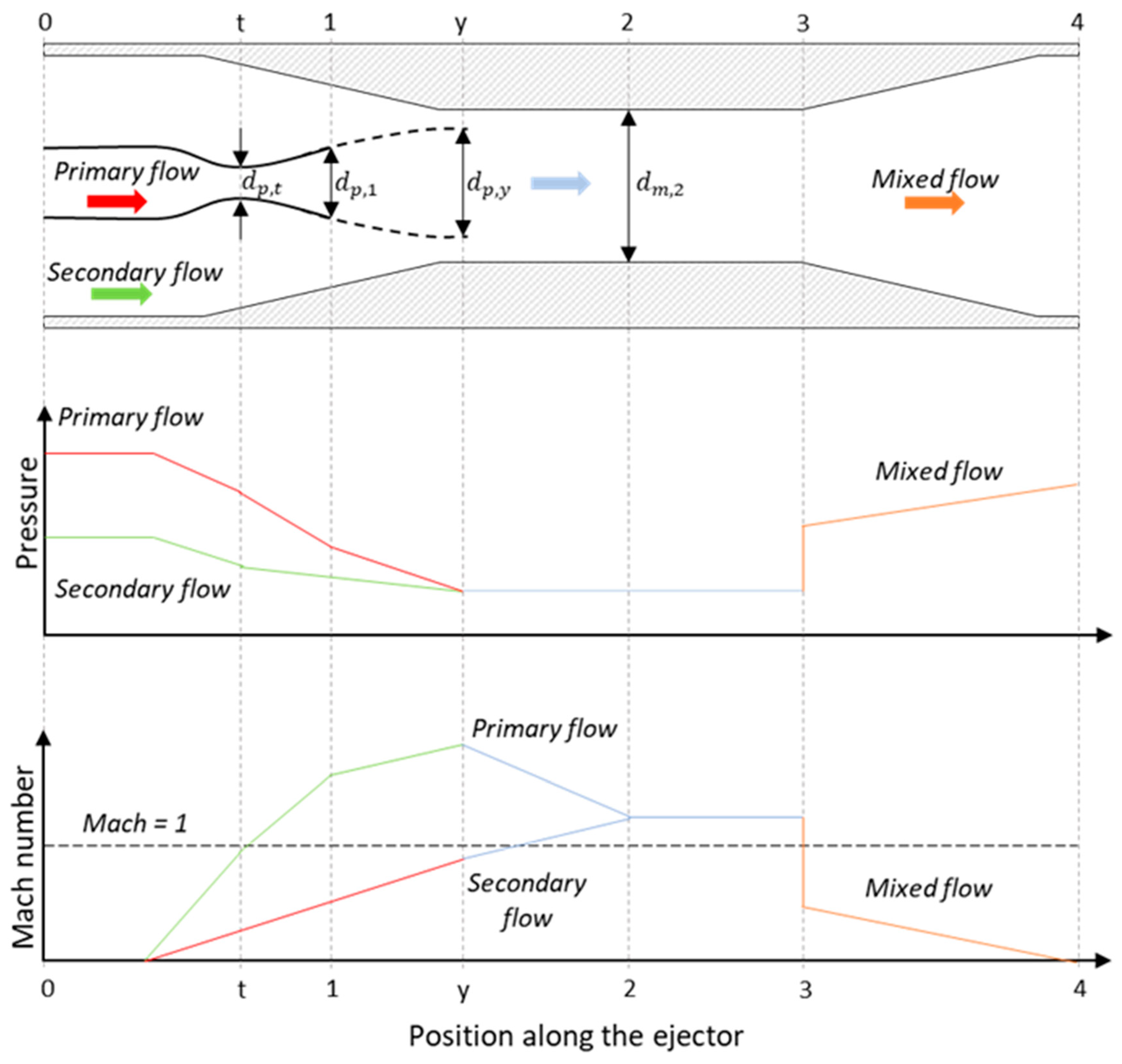
:1. Introduction
2. Model Description
2.1. Ideal Gas Model
2.2. Homogeneous Eulerian Model Combined with Lee Condensation–Evaporation Model
2.3. Wet-Steam Model
3. Methods Section
3.1. Ejector Geometry
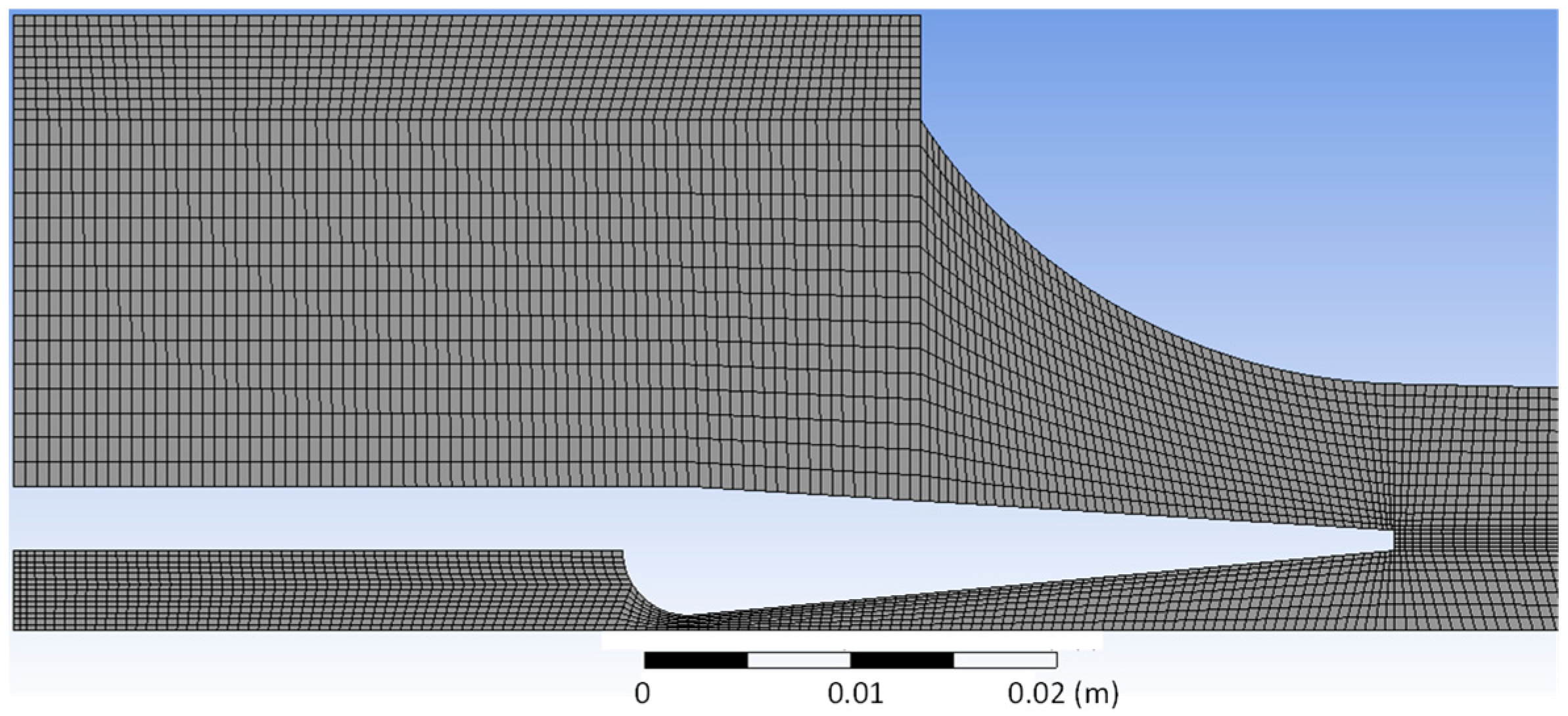
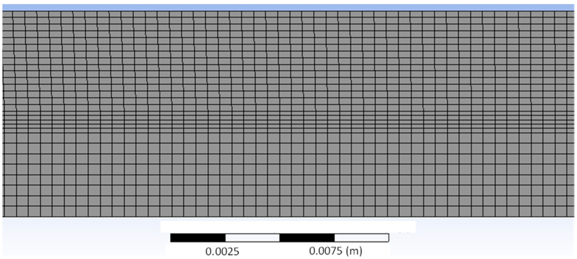
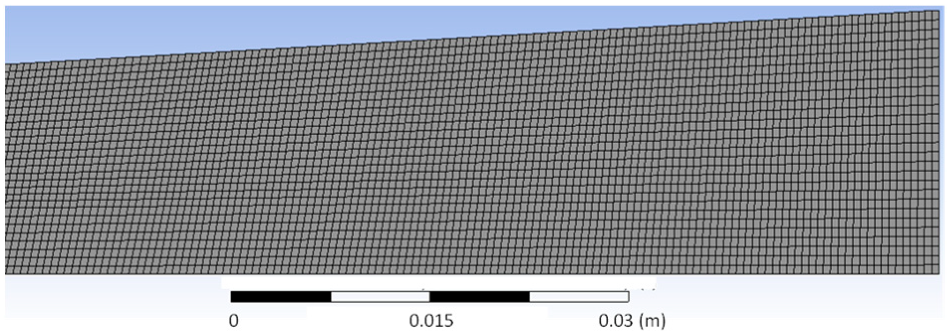
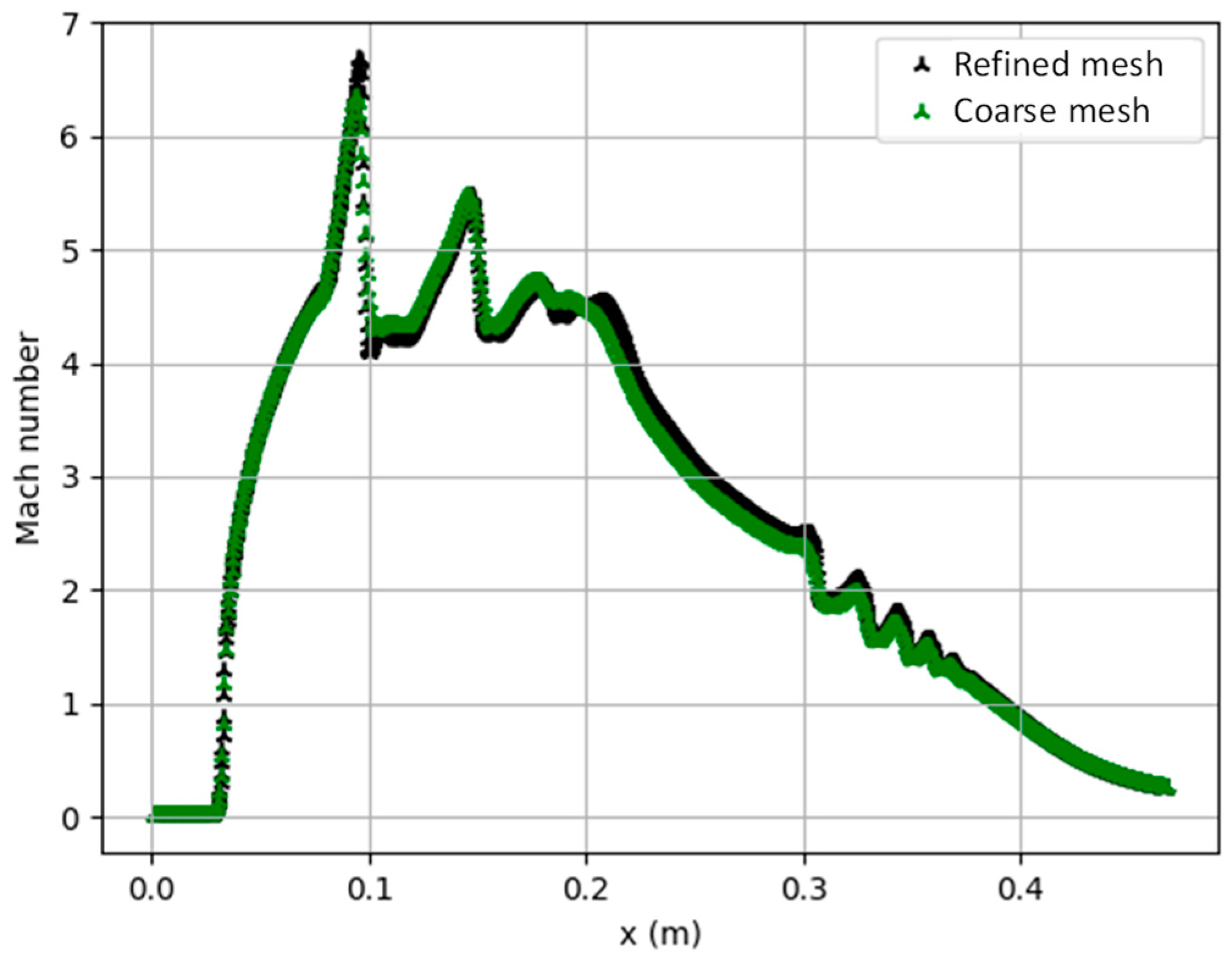
3.2. Meshing and Boundary Conditions
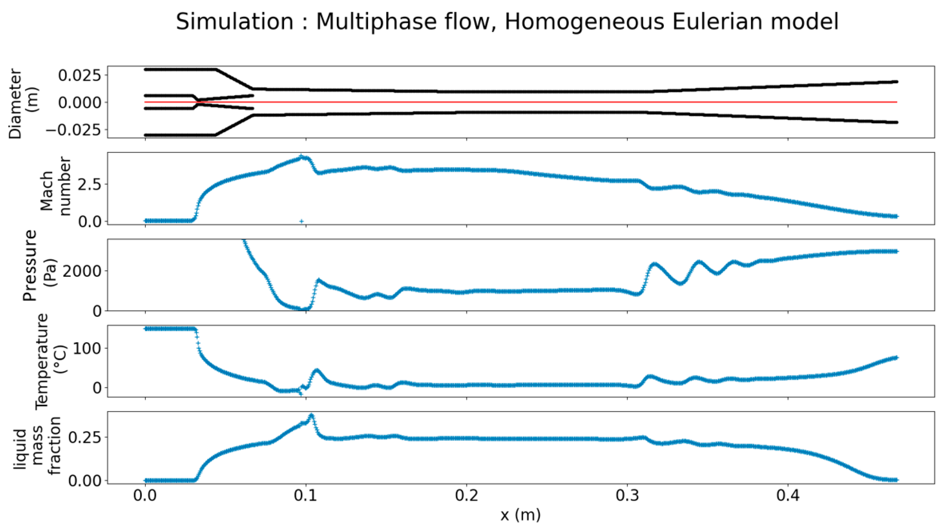
3.3. Calibration of the Coefficients of the Homogeneous Eulerian Model Combined with Lee Condensation–Evaporation Model
4. Results and Discussion
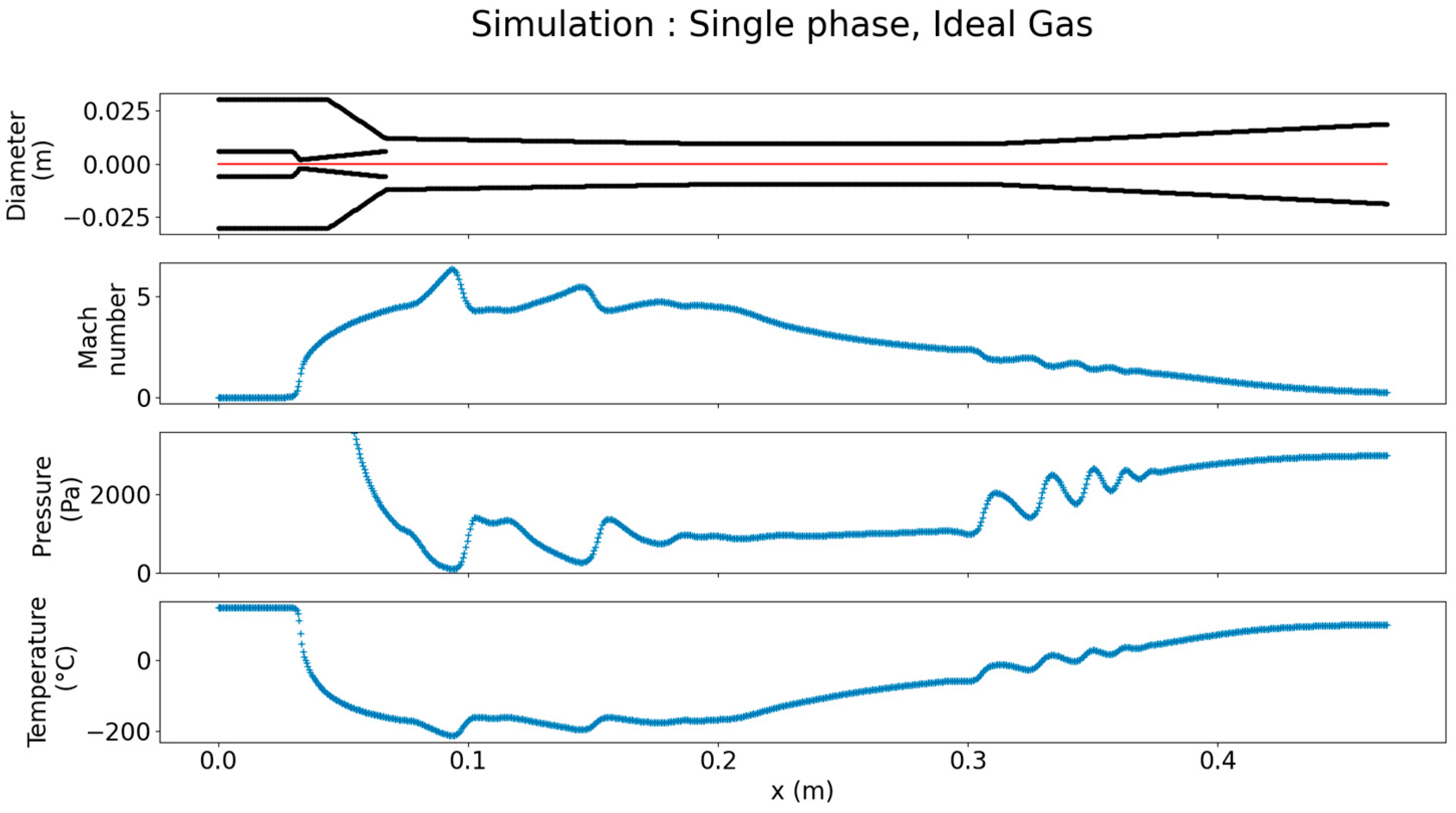
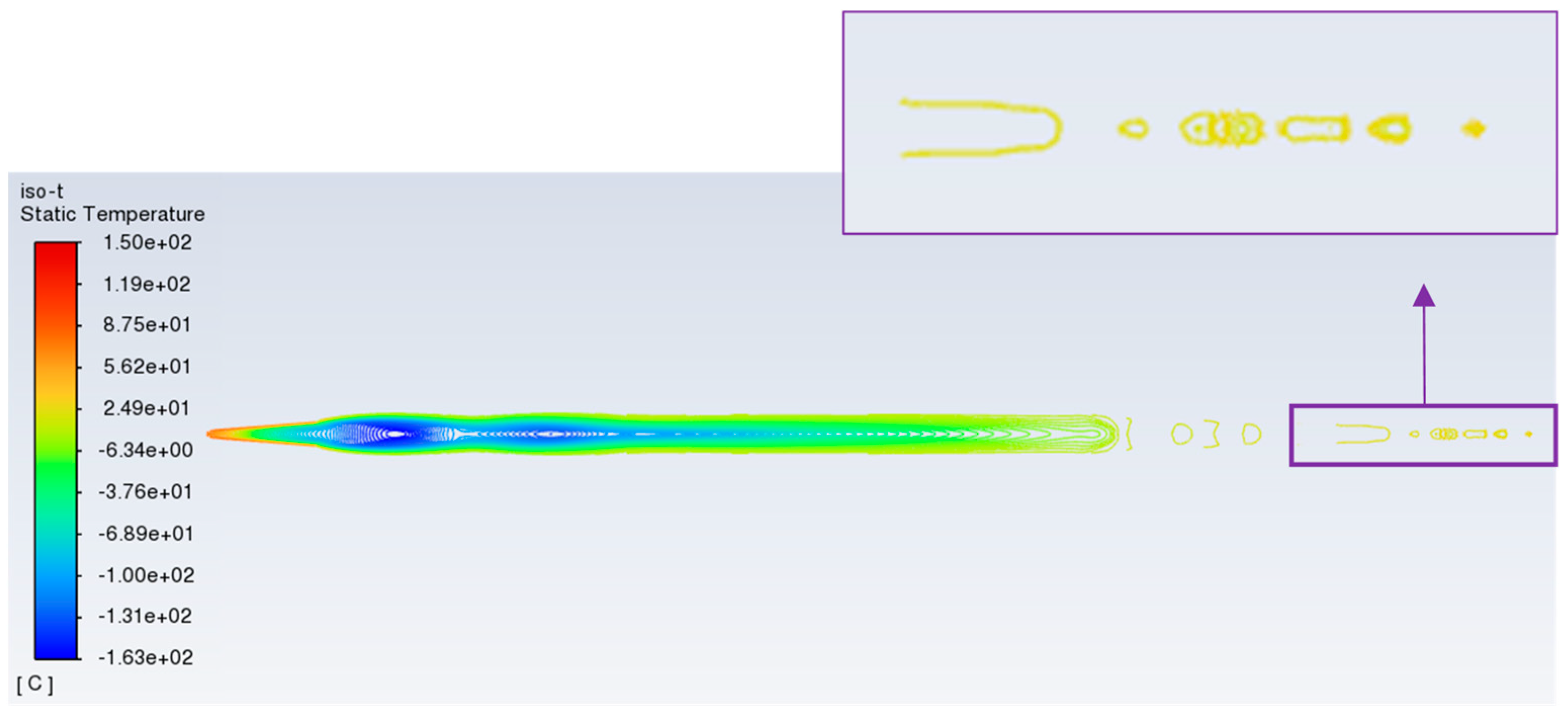
4.1. Temperature Analysis of the Single-Phase Ideal Gas Model
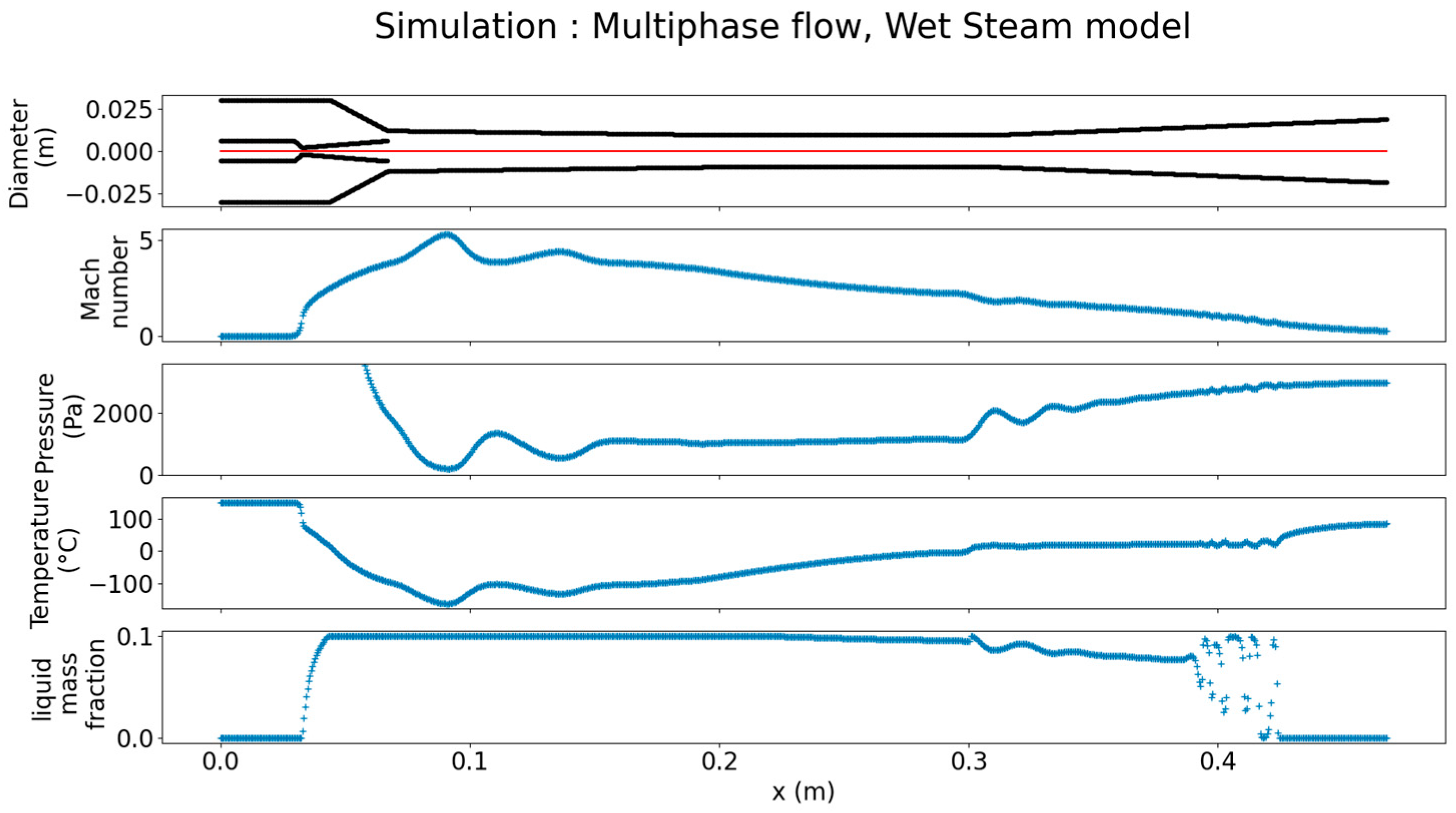
4.2. Temperature Analysis of the Wet-Steam Model
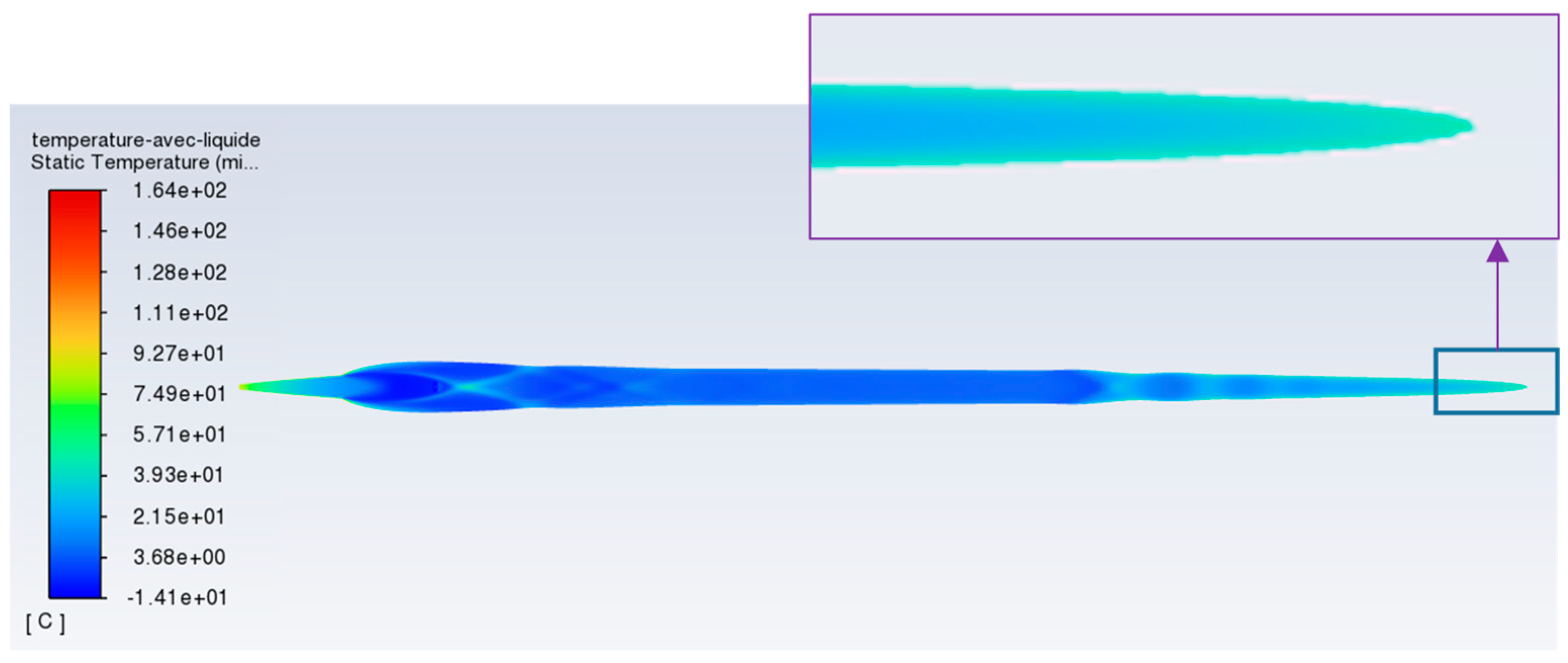
4.3. Temperature Analysis of the Homogeneous Eulerian Model Combined with Lee Condensation–Evaporation Model
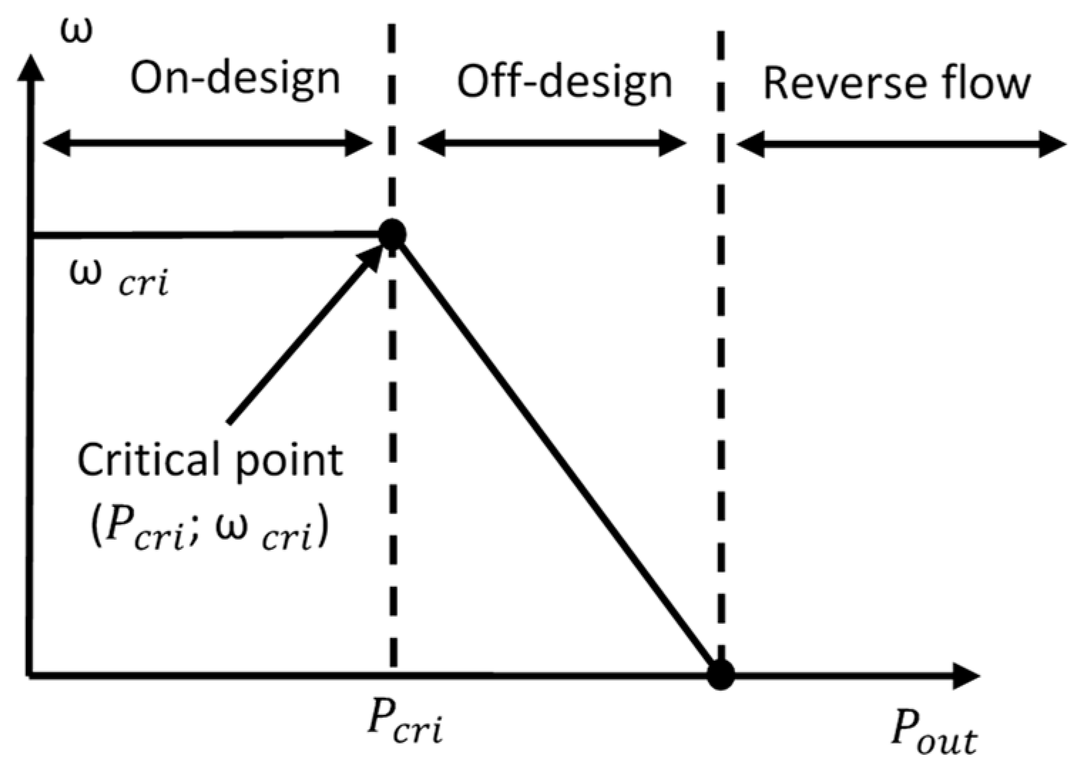
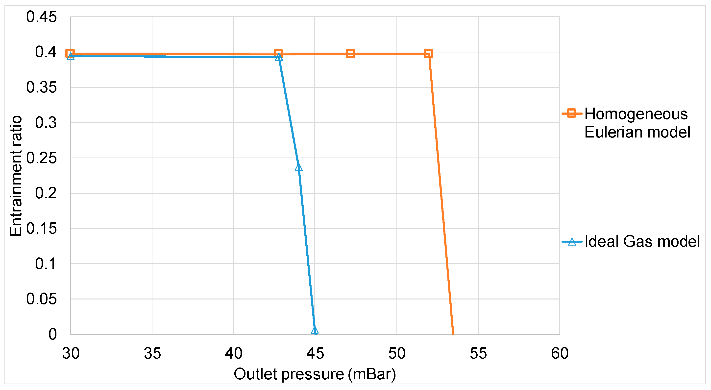
4.4. Comparison of Simulation Entrainment Ratio
5. Conclusions
Author Contributions
Funding
Conflicts of Interest
Nomenclature
| Common letters: | ||
| P | Pressure | Pa |
| T | Temperature | K |
| M | Mach number | - |
| D | Diameter | m |
| Mass flow rate of the primary fluid | kg/s | |
| Mass flow rate of the secondary fluid | kg/s | |
| h | Enthalpy | J |
| k | Turbulent kinetic energy | / |
| v | Velocity | m/s |
| K | Heat transfer coefficient | W//K |
| Turbulent heat transfer coefficient | W//K | |
| Drag force | N | |
| Evaporation mass flow rate | kg/s | |
| Condensation mass flow rate | kg/s | |
| Drift velocity | m/s | |
| C | Lee model coefficient | Hz |
| n | Number of droplets per unit volume | |
| R | Mass generation rate due to evaporation and condensation | |
| I | Nucleation rate | /s |
| Kelvin–Helmholtz critical radius | m | |
| Mass of single molecule | kg | |
| Boltzmann constant | /K) | |
| r | Ideal gas constant divided by molar mass | J/(K.kg) |
| E | Total energy | J |
| Turbulent Prandtl number | - | |
| Re | Reynold number | - |
| CP | The heat capacities at constant pressure | J/K |
| CV | The heat capacities at constant volume | J/K |
| Greek letters: | ||
| ρ | Density | kg/ |
| ω | Entrainment ratio | - |
| ε | Turbulent dissipation rate | / |
| η | Dynamic viscosity | Pa.s |
| μ | Kinematic viscosity | /s |
| Turbulent viscosity | Pa.s | |
| Particles relaxation time | s | |
| β | Liquid mass fraction | - |
| σ | Surface tension | N/m |
| Correction factor | - | |
| Laplace coefficient | - | |
| Volume fraction of phase i | - | |
| τ | Viscous stress tensor | Pa |
| Index: | ||
| c | critical | |
| r | reverse | |
| m | mixture | |
| l | liquid | |
| v | vapor | |
| sat | saturation | |
References
- Voeltzel, V.; Phan, H.T.; Blondel, Q.; Gonzalez, B.; Tauveron, N. Steady and dynamical analysis of a combined cooling and power cycle. Therm. Sci. Eng. Prog. 2020, 19, 100650. [Google Scholar] [CrossRef]
- Godefroy, A.; Perier-Muzet, M.; Mazet, N. Thermodynamic analyses on hybrid sorption cycles for low-grade heat storage and cogeneration of power and refrigeration. Appl. Energy 2019, 255, 113751. [Google Scholar] [CrossRef]
- Elbel, S.; Lawrence, N. Review of recent developments in advanced ejector technology. Int. J. Refrig. 2016, 62, 1–18. [Google Scholar] [CrossRef]
- Meunier, F.; Neveu, P. Convertisseurs thermiques—Machines frigorifiques. Pompes à chaleur. Thermotransformateurs. Froid Ind. 2018, BE 9 734v2, 1–17. [Google Scholar] [CrossRef]
- Braccio, S.; Guillou, N.; Le Pierrès, N.; Tauveron, N.; Phan, H.T. Mass-Flowrate-Maximization Thermodynamic Model and Simulation of Supersonic Real-Gas Ejectors Used in Refrigeration Systems. Therm. Sci. Eng. Prog. 2023, 37, 101615. [Google Scholar] [CrossRef]
- Ruangtrakoon, N.; Thongtip, T.; Aphornratana, S.; Sriveerakul, T. CFD Simulation on the Effect of Primary Nozzle Geometries for a Steam Ejector in Refrigeration Cycle. Int. J. Therm. Sci. 2013, 63, 133–145. [Google Scholar] [CrossRef]
- Bumrungthaichaichan, E.; Ruangtrakoon, N.; Thongtip, T. Performance Investigation for CRMC and CPM Ejectors Applied in Refrigeration under Equivalent Ejector Geometry by CFD Simulation. Energy Rep. 2022, 8, 12598–12617. [Google Scholar] [CrossRef]
- Al-Doori, G. Investigation of Refrigeration System Steam Ejector Performance through Experiments and Computational Simulations. Ph.D. Thesis, University of Queensland, Brisbane, Australia, 2013. [Google Scholar]
- Ariafar, K.; Buttsworth, D.; Al-Doori, G.; Malpress, R. Effect of Mixing on the Performance of Wet Steam Ejectors. Energy 2015, 93, 2030–2041. [Google Scholar] [CrossRef]
- Mazzelli, F.; Giacomelli, F.; Milazzo, A. CFD Modeling of Condensing Steam Ejectors: Comparison with an Experimental Test-Case. Int. J. Therm. Sci. 2018, 127, 7–18. [Google Scholar] [CrossRef]
- Ruangtrakoon, N.; Aphornratana, S.; Sriveerakul, T. Experimental Studies of a Steam Jet Refrigeration Cycle: Effect of the Primary Nozzle Geometries to System Performance. Exp. Therm. Fluid Sci. 2011, 35, 676–683. [Google Scholar] [CrossRef]
- Lee, W.H. A Pressure Iteration Scheme for Two-Phase Modeling; Technical Report LA-UR 79–975; Los Alamos Scientific Laboratory: Los Alamos, NM, USA, 1979. [Google Scholar]


| Mixing Chamber | Ejector Throat | Diffuser | Secondary Fluid Inlet | Primary Fluid Nozzle | |
|---|---|---|---|---|---|
| Length (mm) | 130 | 114 | 180 | 44 | 67 |
| Maximum diameter (mm) | 24 | 19 (constant) | 40 | 46.6 | 7.75 |
| Primary Fluid Inlet | Secondary Fluid Inlet | Outlet | |
|---|---|---|---|
| Type of boundary condition | Pressure inlet | Pressure inlet | Pressure outlet |
| Pressure (Pa) | 476,160 | 1037 | 3000 |
| Temperature (°C) | 150 | 7.5 |
| Single Phase Ideal Gas Model | Single Phase Ideal Gas Model | Wet-Steam Model | Homogeneous Eulerian Model | |
|---|---|---|---|---|
| Solver used | Density-based | Pressure-based | Density-based | Pressure-based |
| ω | 0.463 | 0.394 | 0.456 | 0.398 |
| Relative error with experience (%) | 37.6 | 26.6 | 36.6 | 27.3 |
Disclaimer/Publisher’s Note: The statements, opinions and data contained in all publications are solely those of the individual author(s) and contributor(s) and not of MDPI and/or the editor(s). MDPI and/or the editor(s) disclaim responsibility for any injury to people or property resulting from any ideas, methods, instructions or products referred to in the content. |
© 2024 by the authors. Licensee MDPI, Basel, Switzerland. This article is an open access article distributed under the terms and conditions of the Creative Commons Attribution (CC BY) license (https://creativecommons.org/licenses/by/4.0/).
Share and Cite
Charton, H.; Perret, C.; Phan, H.T. Analysis of Supersonic Flows inside a Steam Ejector with Liquid–Vapor Phase Change Using CFD Simulations. Thermo 2024, 4, 1-15. https://doi.org/10.3390/thermo4010001
Charton H, Perret C, Phan HT. Analysis of Supersonic Flows inside a Steam Ejector with Liquid–Vapor Phase Change Using CFD Simulations. Thermo. 2024; 4(1):1-15. https://doi.org/10.3390/thermo4010001
Chicago/Turabian StyleCharton, Hugues, Christian Perret, and Hai Trieu Phan. 2024. "Analysis of Supersonic Flows inside a Steam Ejector with Liquid–Vapor Phase Change Using CFD Simulations" Thermo 4, no. 1: 1-15. https://doi.org/10.3390/thermo4010001