Simplified Modeling and Experimental Validation of a Combi-Storage Distribution Tank for Seasonal Thermal Energy Storage Systems

Abstract

This study regards the evaluation of the performance of a thermally stratified tank as an intermediate combi-storage tank for a solar-driven residential thermal system coupled to a seasonal energy storage system. In such applications, the efficient operation of this intermediate tank is crucial to the enhanced exploitation of the harvested solar energy and the minimization of heat losses. In this perspective, the development of a dedicated model in TRNSYS software and its validation with experimental results are investigated. With respect to the simulation model’s discretization, it was found that beyond 60 nodes, the benefits to the model’s accuracy are almost negligible. Comparing the experimental data with the simulation’s results, the predicted temperature profile converges accurately to the measured values under steady-state conditions (threshold stabilization period of 1000 s after charging/discharging has occurred). However, the response of the model deviates considerably under transient conditions due to the lack of detailed inertia modeling of both the tank and the rest of the system components. Conclusively, the developed 1D simulation model is adequate for on- and off-design models where transient phenomena are of reduced importance, whereas for dynamic and semi-dynamic simulations, more detailed models are needed.

1. Introduction

The European Union’s (EU) goals for the increased penetration of renewables in new and renovated buildings have increased the interest of the market and academia in residential-scale renewable-based systems [1]. In fact, the EU sub-target of an indicative 1.3% yearly increase of renewables share in heating and cooling in residential buildings, calculated over a period of 5 years starting in 2021, highlights the importance of energy transition in residential applications [2,3]. Among other renewable energy sources, solar thermal energy has several advantages, including its ease of coupling with heating and domestic hot water (DHW) systems and low installation costs owing to its large market [4].

As of 2021, renewable heating is almost solely covered by solid biofuels, accounting for an average of 29.2% of the total space heating loads on an EU basis, based on data from Eurostat [5]. Regarding DHW, 13.9% of the total demand in 2021 was covered by renewables and biofuels [5]. Among other types of renewables, solar thermal energy can offer a relatively cheap solution to cover part of the DHW and space heating loads, resulting in a larger reduction of conventional fossil fuel-based technologies. In order to minimize the thermal spikes and also tackle the time variability of solar energy, thermal energy storage is extensively applied in coupling to solar harvesting systems [6].

Thermal energy storage (TES) systems can be distinguished into three types: sensible, latent, and thermo-chemical storage [7]. In sensible heat storage, there is no phase change in the storage medium. In the simplest configuration, sensible heat storage is realized by a single pressurized tank that is filled with the heat transfer fluid (HTF) that also circulates in the solar collectors. Alternatively, the storage tank can be part of a secondary, intermediate heat transfer circuit that is used for transferring heat from the solar collectors to the consumer/building. In the latter case, the HTF of the primary circuit flows through a helical coil inside the tank and charges it, causing the temperature of the storage medium to increase [8]. Other types of sensible heat storage include underground heat storage, rock beds, and storage using concrete modules [9,10]. In latent heat storage, the storage medium is a phase change material (PCM), which is solidified and melted during charging and discharging phases, respectively [11]. Because of the large enthalpy change associated with phase change, the energy density of latent heat storage systems is much higher compared to that of sensible storage systems, so they can be more compact [12]. Finally, thermo-chemical energy storage is based on a reversible endothermal chemical reaction [13]. The most important advantage of thermo-chemical energy storage is its high storage capacity, which can be several times higher than that of conventional sensible storage systems [14,15].

In most solar-driven residential applications, sensible heat storage is used owing to its simplicity, high market availability, and low costs [16]. Several studies discuss the performance characteristics, modeling aspects, and system integration concepts of sensible storage systems [17,18,19]. Raccanello et al. [8] evaluated different order models for several types of single-tank storage systems to assess the reliability of simplified modeling approaches for integrating storage tank models into more complex systems without severely affecting the computational cost. Tian and Zhao [20] conducted a detailed review of different types of solar thermal collectors and high-temperature thermal energy storage systems.

Ismaeel and Yumrutas [21] simulated the performance of a solar-assisted heat pump connected with an underground thermal energy storage system for wheat drying. For a defined solar field area, the storage tank was sized in order to retain a satisfactory temperature range throughout the year. Syed et al. [22] experimentally evaluated a solar absorption cooling system coupled with a 2 m³ stratified storage tank in the city of Madrid, Spain. The operation of a 35 kW nominal capacity absorption chiller, driven by a solar field of 50 m² flat plate collectors (FPC), was prolonged by the use of the storage tank, leading to a total daily operation lasting approximately 7.3 h. Karim et al. [23] evaluated the performance of stratified storage tanks for heating/cooling applications and concluded that tanks with higher height-to-diameter ratios tend to reduce mixing and thus reduce heat losses. In the same direction, Pintaldi et al. [24] evaluated the energetic performance of sensible and latent heat storage scenarios for solar cooling applications. The analysis found that, for the evaluated scenarios, a minimum specific collector area of 2 m² per kW of cooling capacity is required for achieving solar fractions higher than 50%. Jung et al. [25] assessed control strategies for the optimal operation of a heating system consisting of a heat pump and a thermal storage tank for use in Seoul, South Korea.

Çomaklı et al. [26] evaluated the influence of storage tank sizing on solar water heating systems. The analysis revealed that an increase in the storage tank capacity may enhance the solar collector’s efficiency, but simultaneously, as expected, the average water temperature in the tank decreases. Therefore, an optimal design exists per case; for the scenario of the Turkish DHW standards, a storage tank volume to solar field area ratio of 50–70 L/m² was defined as optimal by the authors of this study. Similarly, Li et al. [27] optimized the storage tank capacity for integration in a solar heating system to be installed in a typical building in Xi’an, China. The optimal storage tank volume to solar field area ratio was determined to be 10–20 L/m².

The aforementioned systems focused mostly on short-term storage, which is a totally feasible solution for regions with high solar irradiance, even in the colder months of the year. However, in colder climates (central and northern Europe), solar irradiance is mostly available during hotter periods of the year, and thus there is very limited concurrence with space heating loads. Therefore, the exploitation of solar energy in such regions is only possible with the implementation of seasonal thermal energy storage (STES).

Despite several studies on latent and thermo-chemical storage, sensible storage is the only economically viable solution for STES [28]. One of the first commercial solar-driven STES was built in Hamburg in 1996 [29]. The system was based on an underground concrete tank filled with 4500 m³ of water, achieving in design conditions a solar fraction of 49%. Since then, several studies have been conducted, both through simulations and experiments on STES systems. Terziotti et al. [30] simulated in TRNSYS the performance of a sand-based STES for a five-story student housing complex located at Virginia Commonwealth University, USA. The simulations revealed that in a building with lower heating loads, the solar fraction reached a value of up to 91%. Sweet et al. [31] modeled in TRNSYS a solar-powered underground STES system for a residential application in Richmond, Virginia, USA. By evaluating different floor areas of the tested building, it was found that the optimal sizing of the investigated system resulted in a reduction in conventional system consumption of up to 77%. Antoniadis and Martinopoulos [32] conducted a study in TRNSYS to evaluate a solar-driven system using a STES for a 120 m² single-family building in Thessaloniki, Greece. The system was able to reach a solar fraction of 52.3% with respect to the heating loads. Hailu et al. [33] reported a reduction of more than 40% in the heating loads by the implementation of a solar-driven STES in a two-story house located in Alaska, USA. Hesaraki et al. [34] evaluated a STES coupled with a heat pump connected to low-temperature space heat emissions for a single-family building located in Stockholm, Sweden. The analysis showed that the optimal ratio of storage capacity to solar field area is approximately 5 m³/m². Li et al. [35] simulated a solar thermal heat pump system coupled with STES to cover the space heating and DHW loads of a six-story dorm building with a total area of 2252 m², located in Beijing, China. The proposed system was found to improve the monthly coefficient of performance (COP) by 12.8% compared to a conventional heat pump system. Drosou et al. [36] reported the performance of a solar-driven cooling/heating system coupled with an underground STES. The system is used to cover the space heating and cooling loads of a 427 m² office building located in Athens, Greece. The measured solar fraction of the system, which uses an absorption chiller and a conventional heat pump, was as high as 70%.

Gabrielli et al. [37] carried out an optimization procedure to size multi-energy systems coupled with STES by implementing two novel mixed integer linear program models. The proposed methodology was evaluated for the case of a residential application, combining options of seasonal storage technologies, including STES, hydrogen, and battery storage. In fact, the analysis showed that for larger emission savings, thermal storage reported optimal performance only covering the peak loads, while hydrogen seasonal storage was the optimal technology to handle the base loads of the residential building on an annual basis. McKenna et al. [38] assessed the techno-economic performance of a STES for a typical German residential district. The analysis showed that a 60% renewable heat supply fraction does not significantly increase costs and is therefore viable as a solution.

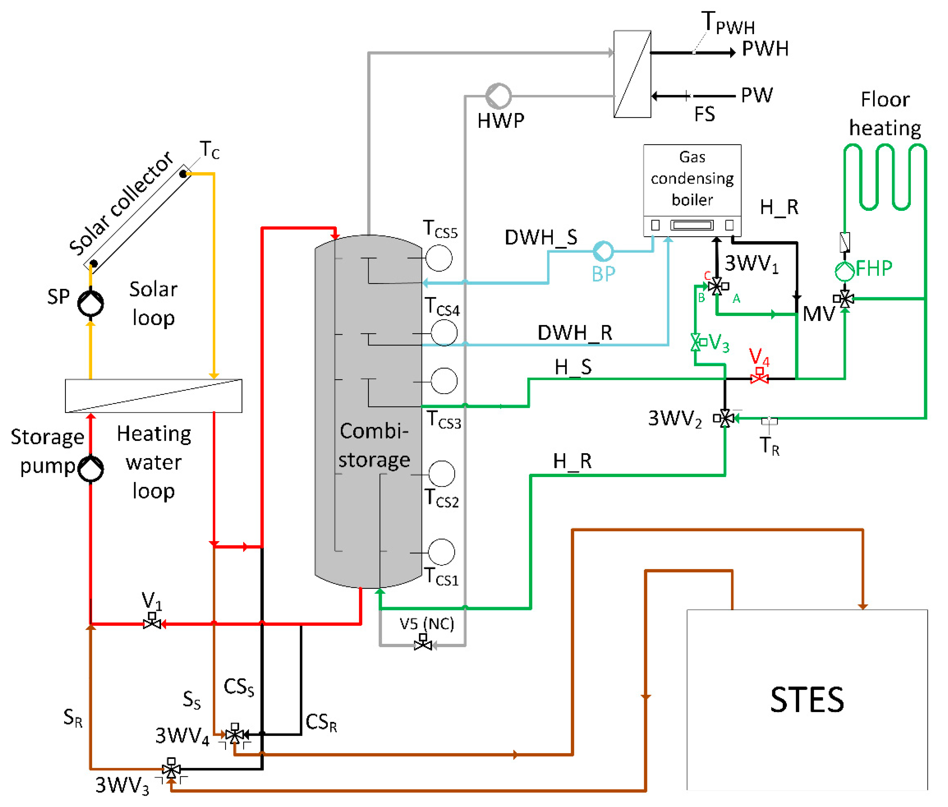
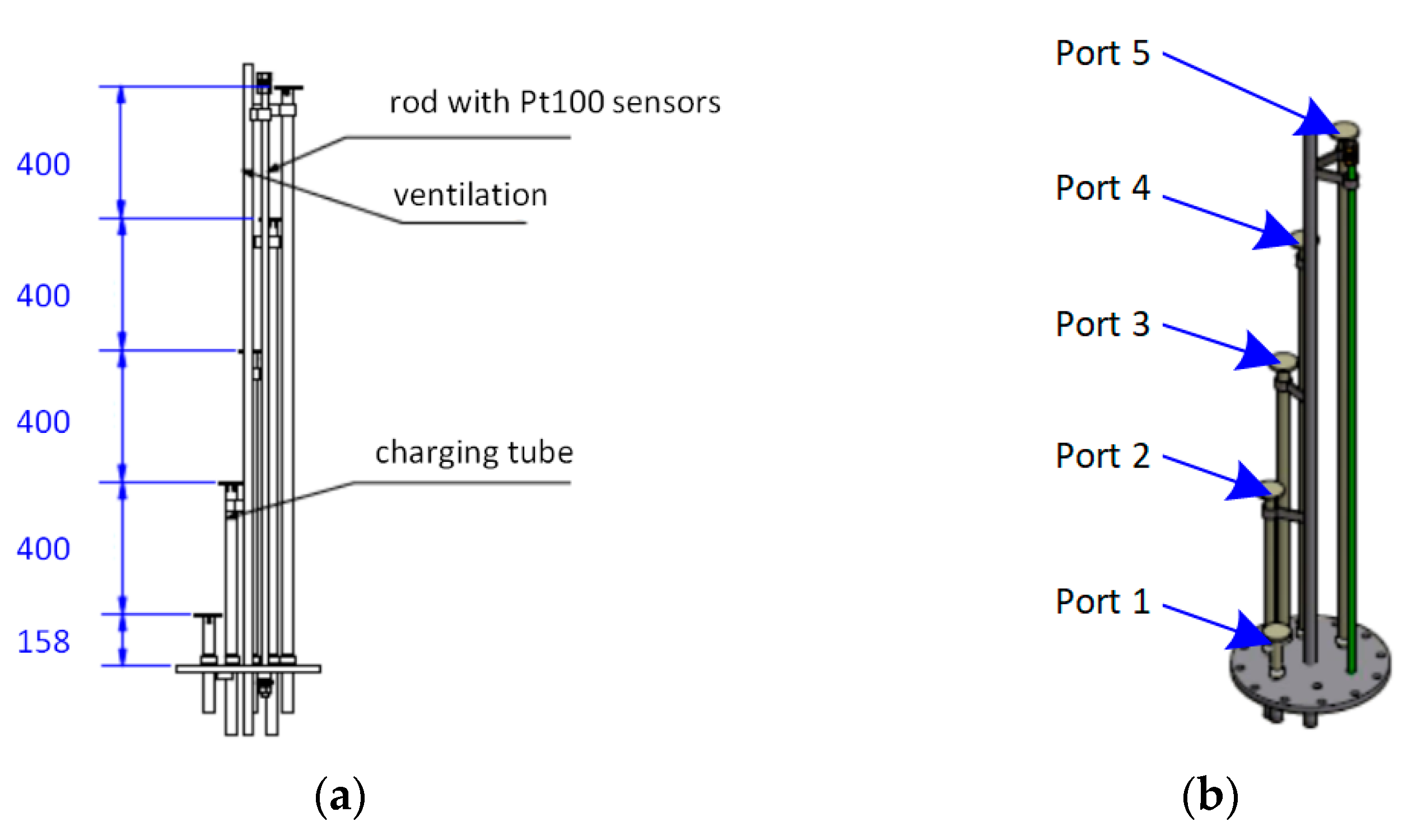
In this study, a thermal energy storage system driven by evacuated tube collectors (Figure 1) is investigated both numerically and experimentally. The distribution of the available solar heat and the heat stored in the STES is realized via a residential heating and DHW distribution system based on a thermally stratified water tank. The tank is working as a diurnal thermal energy storage device, coupled with a natural gas boiler. The solar heat is used to charge the Combi storage tank and/or the STES. Space heating is provided to the building through a floor heating system, while DHW is supplied via a dedicated heat exchanger. STES is used either as a backup or to cover peak loads on days with inadequate solar irradiance. A condensing gas boiler operates as a backup thermal energy source to ensure thermal comfort at any time of the year.

The prediction of the performance of the stratified tank that is coupled with the distribution system is crucial for the overall system efficiency. For this purpose, a simulation model was developed in TRNSYS 18 [39] along with an experimental test rig. The experimental results are also used to calibrate the simulation model and assess its accuracy.

Thermal modeling of sensible heat storage tanks with TRNSYS software has been extensively investigated in the literature [40]. The novelty of this study, compared to the existing literature, is the use of experimental data for verifying the performance of the system, which is also based on a non-standard component for modeling the effect of tank stratification. Minimize the simulation errors related to thermal nodes close to the inlet/outlet ports of the stratified tank. Furthermore, most of the existing studies on sensible storage have not considered cases including seasonal storage systems coupled with underfloor heating, which is the scope of the investigated concept.

In that context, this study aims at presenting the development, experimental evaluation, and calibration of the employed simplified stratified tank model parameters in coupling with specific thermal loads associated with the respective DHW and heating demands as defined by the EU standards. As a result, a detailed overview of the model’s accuracy during different mixing, charging, and discharging phases is thoroughly investigated.

2. Materials and Methods

2.1. Definition of Experimental Test-Rig

In order to simulate the energy demand of a residential nearly zero energy building (nZEB), a dedicated test rig was developed at the Laboratory of Steam Boilers and Thermal Power Plants of the National Technical University of Athens, Greece. The DHW and space heating loads are simulated using two heat exchangers connected to a heat sink (Figure 2). A gas condensing boiler is used to charge the combi-storage tank, emulating the solar collectors and STES (in discharge mode). Depending on the available water temperature, space-heating hot water can be supplied solely from the tank, using the tank’s stored heat and a possible recharging via the boiler, or solely from the boiler, bypassing the tank, to achieve the necessary temperature for thermal comfort. More specifically, in cases of heating demand and no stored energy in the space heating section of the tank (Figure 2), if the boiler is not used for charging the DHW section, the heating demand is met using the natural gas boiler for reheating (brown line in Figure 2) or directly as the main heat source (blue line in Figure 2). For this reason, a modulating boiler was selected for this system.

The switching between the different heating operational modes is achieved using 3-way changeover valves, while the temperature of the delivered water for space heating is ensured using a 3-way mixing valve controlled with a PID control. In addition, in each of the three loops in Figure 2, namely the DHW, heating, and charging loops, a different circulation pump is used according to the energy demand. DHW and heating demand profiles are used according to EU standards [41] and residential nZEB simulations [42,43]. As shown, the solar collectors were not coupled with the test rig to avoid the time variability of solar heat for the needs of the conducted experiments.

An overview of the actual test rig layout is depicted in Figure 3. In the following subsections, data are listed on the specific components used in the test rig.

2.2. Combi-Storage Tank

The combi-storage water tank is thermally stratified and works as temporary thermal energy storage in the form of hot water. The combi-storage tank capacity is equal to 535 L, with its main external dimensions shown in Figure 4. For the thermal stratification to be preserved while at the same time minimizing heat losses, the tank needs to be highly insulated. This is achieved by a vacuum-wall-insulated tank. This way, the thermal losses via conduction and convection are minimized due to the absence of air, and the radiant losses are predominant.

The tank is double-walled; between the inner and outer walls, high-efficiency non-removable vacuum insulation is included, making the buffer tank suitable to operate in outdoor conditions. The tank is supported by metal feet, while flanges extend from the bottom, allowing access to all five different ports. The insulation space is filled with thermal radiation absorber material. The absolute pressure is <<100 Pa, preventing aging effects on the insulation value. The pressure can rise slightly in 5/10 years due to the long-term diffusion effects. A pressure higher than 1000 Pa could lead to higher thermal losses. The technical data of the combi-storage tank are summarized in

Table 1. Technical specifications of the Combi-storage tank.

Property	Value
Maximum operating pressure (bar)	3
Maximum operating temperature (°C)	95
Total height (mm)	2555
External tank diameter (mm)	1000
Inner tank volume (L)	535
Inner tank diameter (mm)	650
Insulation thermal conductivity (W/mK)	0.008

. There are five available ports, numbered as shown in the schematic of Figure 2, all entering vertically from the bottom of the tank to different heights of its interior, with the corresponding dimensions of Figure 5. At the same height as each port, there is a Pt100 thermal resistance sensor to ensure accurate measurement of the temperature in each subcircuit of the system.

The highest port (#5 according to Figure 2), corresponding to the highest available temperature, is used for DHW supply, while ports #3 to #4 provide water to and from the boiler, respectively, to charge the DHW section of the tank. Port #2 is used for supply to the heating system at temperatures of approximately 38 °C, while both DHW and heating cold consumption return streams enter port #1. The heating loop (ports #2 to #1) is also used to charge the lower section of the tank using the boiler. This test rig setup is also modeled and studied numerically, as described below.

2.3. Condensing Gas Boiler

As mentioned above, a modulating boiler was required to operate at two different temperature setpoints. The size of the boiler was dictated by the need to cover a maximum capacity of 18.8 kW for DHW production and 10 kW for space heating. To achieve higher efficiencies, the gas boiler was selected to be a condensing one. A condensing boiler recovers the latent heat of evaporation from the water vapor in the exhaust gas, which would otherwise have been wasted [44]. The relatively small temperature differences that were required for the considered application of underfloor heating simulation indicated the need for a combi-boiler with a lower limit of its power capacity being as small as permitted by the commercially available products.

Following a market search, the boiler chosen was the natural gas condensing boiler “Riello Residence Condens 25KIS e” [45]. The boiler can achieve reduced thermal power for DHW production of 3.3 kW and reduced thermal power for heating mode equal to 3.8 kW for a temperature rise from 30 K to 50 K. The nominal thermal power for DHW and space heating is 26.3 kW (average nominal thermal power for different DHW modes) and 21.2 kW (50°–30°), respectively.

The boiler’s control is designed in such a way to give priority to the DHW application. This is realized via a flow switch, activated when there is water flow in the boiler-DHW circuit. The selected model has a secondary integrated heat exchanger to generate DHW, which is a characteristic of the KIS product series. On the other hand, in heating mode, hot water from the primary heat exchanger is heated by the burner and circulated by the internal boiler circulator. In order to avoid excessive pressure, an expansion vessel is built into the hydraulic system of the boiler. In addition, for safety reasons, the circuit has an automatic bypass loop activated by a pressure switch. The heating and DHW inlet temperatures, as well as the heating outlet temperature, are monitored using NTC thermistors.

2.4. Heat Exchangers and Auxiliary Equipment

The heat exchangers were sized based on the inlet and outlet temperatures for both the hot and cold sides, and thus the respective heat duty of each one. In the case of the DHW heat exchanger, the DHW demand profile was estimated based on cycle no. 2, as described in the European Standard [41]. More data on the considered loads based on the European Standard are provided in the Appendix A of this study. Based on the data in

Table A1. Energy needs and flow rates for different types of DHW demand are based on [41].

No.	Start (hh:mm)	Energy Need (kWh)	Type of Delivery	ΔΤ Desired (K) during Tapping	Min. ΔΤ (K) @ Start of Counting Useful Energy
1	07:00	0.105	Small		15
2	07:17	1.400	Shower		30
3	07:30	0.105	Small		15
4	08:00	0.105	Small		15
5	08:15	0.105	Small		15
6	08:30	0.105	Small		15
7	08:45	0.105	Small		15
8	09:00	0.105	Small		15
9	09:30	0.105	Small		15
10	10:30	0.105	Floor Cleaning	30	0
11	11:30	0.105	Small		15
12	11:45	0.105	Small		15
13	12:45	0.315	Dish Washing	45	0
14	14:30	0.105	Small		15
15	15:30	0.105	Small		15
16	16:30	0.105	Small		15
17	18:00	0.105	Small		15
18	18:15	0.105	Household cleaning		30
19	18:30	0.105	Household cleaning		30
20	19:00	0.105	Small		15
21	20:30	0.735	Dish Washing	45	0
22	21:15	0.105	Small		15
23	21:30	1.400	Shower		30
Total		5.845

and

Table A2. DHW type and required flowrate for a temperature rise of 45 K, based on [41].

Type of Tapping	Energy (kWh)	Hot Water Flow Rates (L/min)
Household cleaning	0.105	3 ± 0.5
Small	0.105	3 ± 0.5
Floor cleaning	0.105	3 ± 0.5
Dish washing	0.315	4 ± 0.5
Dish washing	0.420	4 ± 0.5
Dish washing	0.735	4 ± 0.5
Large (cycle no 1)	0.525	4 ± 0.5
Shower	1.400	6 ± 0.5
Shower (cycles no 4 and no 5)	1.800	6 ± 0.5
Bath	3.605	10 ± 0.5
Bath cycle no 4	4.420	10 ± 0.5
Shower and Bath (cycle no 5)	6.240	16 ± 0.5

, the heat duty of the DHW heat exchanger was estimated for the worst-case scenario (largest power demand). The largest power demand corresponded to a temperature rise of 45 K at a 6 L/min flowrate, which is approximately equal to 18.8 kW.

In the case of the space heating heat exchanger, the tank side inlet temperature is set at 38 °C and the outlet at 28 °C, with a maximum rated power of 10 kW based on typical nZEB building simulations [43,46]. Due to the small size of this power demand and the high flow rates in the heat exchanger, larger inlet/outlet ports were preferred to avoid large pressure drops. The heat exchanger duty was estimated at 10 kW with a temperature difference of 10 K at a nominal flow rate of 0.24 L/s on the hot (tank-heat exchanger) side.

With respect to the three circulator pumps used in the circuits connected to the combi-storage tank (see Figure 2), namely the domestic hot water pump (DHWP), the hot water from the boiler pump (HWBP), and the space heating pump (SHP), all were the same commercial model, Grundfos UPS2 32-80 180, working at different design points.

2.5. Measuring Equipment

With respect to the measuring equipment, five Pt-100 three-wire resistive temperature devices (RTD) thermometers were embodied by the tank manufacturer at the same heights with the respective ports of Figure 4 in order to monitor the temperature of the combi-storage tank (denoted in Figure 2 as T₁, T₂, T₃, T₄, and T₅). Additionally, in the pipelines connected to the heat exchangers and the gas boiler, a total of four additional three-wire Pt-100 class A RTDs were implemented with a transmitter of 4–20 mA output (denoted in Figure 2 as T₆, T₇, T₈, and T₉). The uncertainty of each sensor at the nominal operating temperatures is equal to ±(0.15 + 0.2% × MV) °C, where MV is the measured value plus ±0.2 °C due to transmitter error. With respect to water flow measurements, three identical ultrasonic flow meters were used with a maximum allowable flowrate of 0.78 L/s, model Belimo FM020R-SZ (denoted in Figure 2 as FM₁, FM₂, and FM₃). The flowmeter’s output was in the form of a 0.5–10 V voltage output with a measuring accuracy of 2% of the measured value. Pressure drops related to the used heat exchangers were measured via pressure transducers, with a rated accuracy of 2% at maximum measurable pressure (3.44 bar).

Table 2. Technical specifications of measuring equipment.

Property	Value	Unit
Temperature Sensors
Type	Pt100 RTDs
Measuring range (min…max)	−50…80	°C
Output signal (min…max)	4…20	mA
Diameter	6	mm
Class	A	-
Uncertainty	±(0.15 + 0.2% × MV)	°C
Flow sensors
Type	Ultrasonic flowmeter
Model	Belimo FM020R-SZ
Maximum measurable flow (full scale)	0.78	L/s
Pressure drop at full scale	13	kPa
Output signal (min…max)	0.5…10	V
Measuring accuracy and flow	±2% of measured value
Flow Measurement Repeatability	±0.5%
Minimum flow measurement	0.0078	L/s
Ambient temperature (min…max)	−30…50	°C
Pressure sensors
Measuring range pressure (min…max)	0…3.44	bar
Model	Belimo 22WP-514
Accuracy	<±2% at full scale
Output signal (min…max)	0.5…10	V
Maximum response time	2	ms

lists additional specifications for the measuring equipment aforementioned.

2.6. Heat Sink and Back-Up Heating System Modeling

The two tanks in Figure 2, which are used as heat sinks to simulate the DHW and space heating loads, were modeled using Type 534 of the TESS library [47], without any heat exchanger. Each tank had a capacity of 25.5 m³. Owing to their large thermal inertia and low volumetric flowrates, fully mixed tanks were assumed, and thus each tank was modeled with a single node. The model parameters are listed in

Table A5. Simulation Parameters for TESS Type534-NoHX used for the lab thermal storage model.

Property	Value	Unit
Storage Height	5.64	m
Storage Volume	25.5	m3
Specific Heat	4.18	kJ/kgK
Density	998	kg/m3
Fluid thermal conductivity	2.2	kJ/h/m/K
Loss Coefficient (Top, Bottom, Edge)	5	kJ/h/K
Nr of nodes	1	-

of the Appendix A. The thermal losses were calculated based on the ambient temperature, derived from a Meteonorm [48] weather file for the city of Athens, Greece (WMO id 167140, station Athinai).

With respect to the combi-gas boiler, it was simulated using the standard Type 700 “simple boiler with efficiency inputs” component. The maximum temperature of the boiler was set equal to the DHW setpoint of 65 °C, while the respective setpoint of the space heating mode was set at 38 °C.

2.7. Demand Profiles Modeling

The space heating profile is regulated, as stated above, at 38 °C via a mixing loop before the respective heat exchanger. The supply temperature controller used is modeled after a Type 115 controller. The space heating profile, which was used for the respective tests, was switched on arbitrarily and continued its operation until a 5 kWh heat gain was recorded on the cold side of the space heating heat exchanger.

The DHW profile was modeled based on the Type 14 “forcing function water draw.” In order to ensure a step function in TRNSYS, independently of the time step, two Type 14 components were used and added in an equation to create the complete DHW demand profile. The three-way mixing valves used in the system were modeled with the Type 11d component, while the three-way diverting flow valve was modeled with Type 11f. Finally, all pumps were modeled using Type 114 single-speed pumps. An overview of the global system’s setup in TRNSYS 17 is shown in Figure 6.

3. Results and Discussion

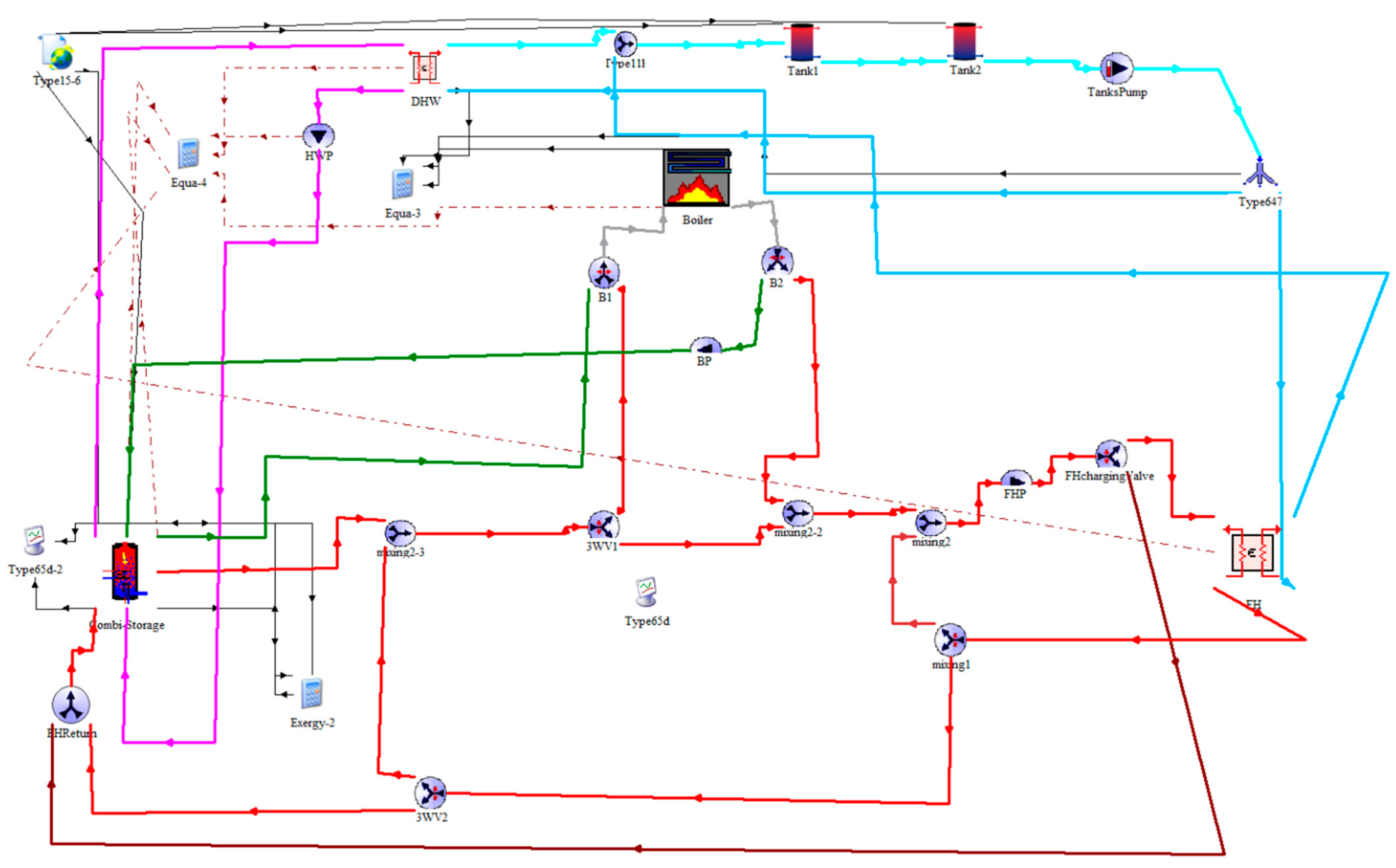
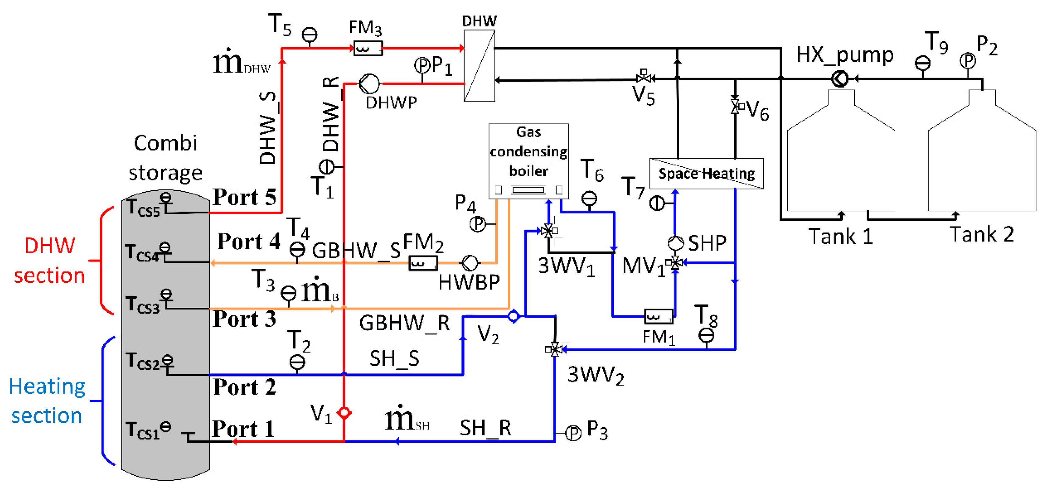
Regarding the control strategy, it was realized with an equation component. The control signal of the boiler’s pump is generated by a Type 1502 thermostat component by comparing the temperature estimation, T_CS4, with a setpoint of 45 °C. During the periods that the HWBP (see Figure 2) is operating, the three-way valves are rerouting the flow to bypass the boiler. On the contrary, when the HWBP is out of operation, the control of the three-way valves follows the actual system’s operational strategy.

For the charging of the lower parts of the combi-storage tank, which are used for the space heating loads, a dedicated directing valve is used. During periods with no DHW and space heating loads, and while the HWBP is off, the control of the three-way valves directs the flow towards the boiler and then bypasses the space heating heat exchanger to feed the heated flow in the lower parts of the tank. This charging procedure continues until T_CS2 reaches the desired setpoint of 45 °C. All different setpoint cases are saved in an equation component, and each dedicated setpoint is used as input for the boiler component, according to the respective mode of operation.

The scope of the experimental test rig was twofold. Firstly, it was developed to assess the potential of the combi-storage tank for efficiently storing heat at different temperature levels and covering the heating and DHW loads of a building. Secondly, the sets of experiments and their results were used to evaluate the accuracy of the non-standard TRNSYS component towards its implementation in more complicated systems.

It is here noted that the error analysis of the experimental results is out of the scope of this study. The analysis regards the comparison of the simulated temperature levels with the values directly measured by the temperature sensors. Hence, the uncertainty of the experimental results is directly related to the accuracy of the temperature sensors reported in Section 2 and is not propagated through further calculations. As regards the measured water flow rate values, these are given as an input to the simulation model alongside the uncertainty of the respective sensors. With respect to the simulations, they were conducted with a relative convergence tolerance of 0.1% for all model variables.

3.1. Nodes’ Number

As already stated, the non-standard component Type 340 was used for the combi-storage tank simulations, which is based on the ‘MULTIPORT’ store model [49]. The modeling of the tank’s stratification followed the isothermal nodes approach, dividing the tank into a number of N fully mixed finite volumes and applying respective energy balances [50]. The nodal approach was preferred over the plug flow approach, as it better simulates the tank’s thermal stratification, according to the study of Allard et al. [51].

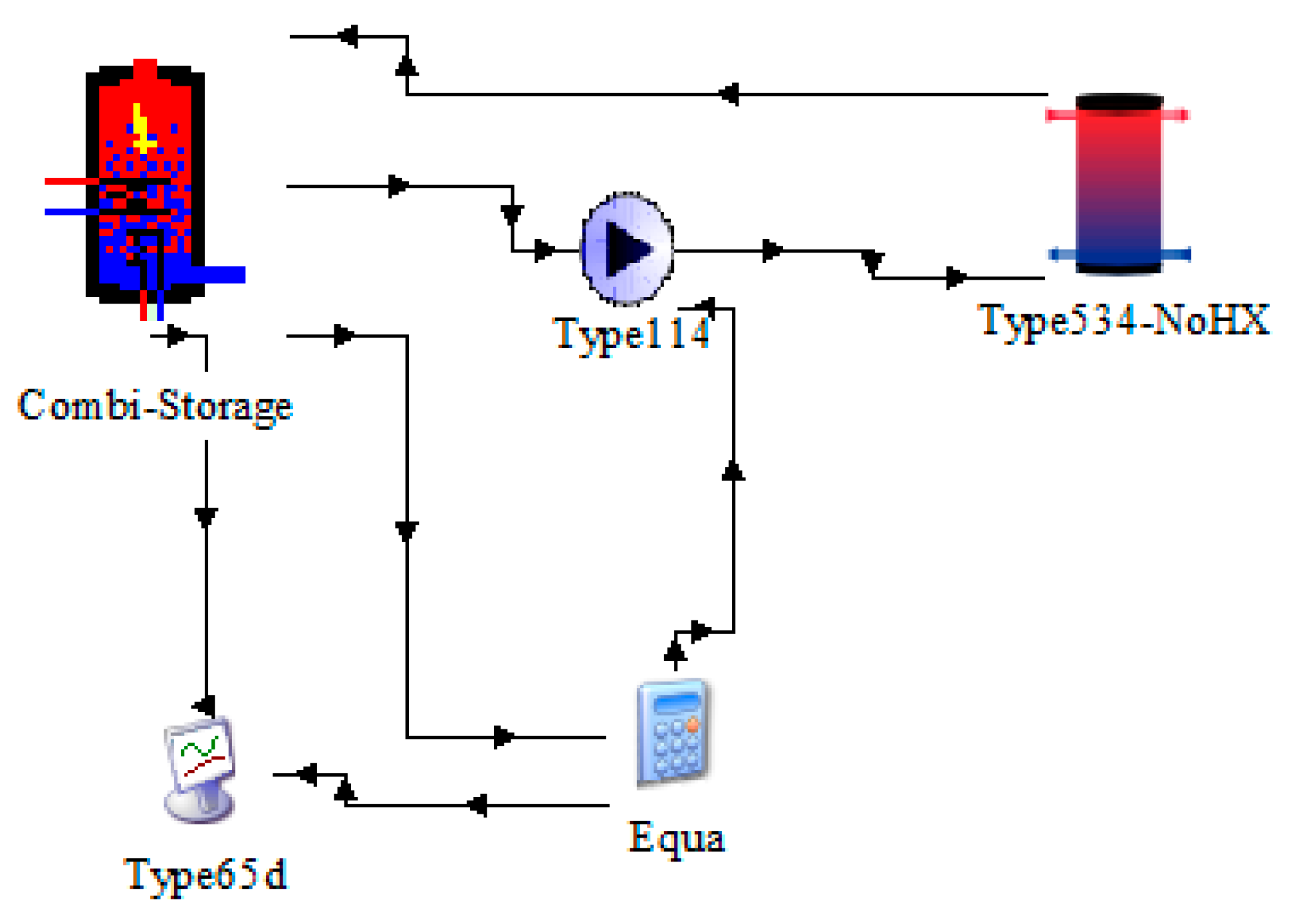
The first step in the experimental evaluation of the developed model concerned the selection of the node number to be used in the model. In order to simulate the loads interacting with the combi-tank in the test rig of Figure 2, a constant temperature source was implemented in TRNSYS via a Type 534 cylindrical storage tank without any heat exchangers considered [52]. The node number of the cylindrical storage tank was set at 1, corresponding to a fully mixed tank, while the heat loss coefficient was set at 0. The tank’s volume was assumed to be twenty times larger than the combi-storage tank’s volume. The selection of such a large theoretical volume allowed for a very high thermal inertia of the cylindrical tank compared to the evaluated combi-storage tank, and thus a constant supply temperature defined during simulation. A type 114 constant-speed pump was introduced to set the flow towards the combi-storage tank. An overview of the simplified combi-storage tank model for the nodes’ evaluation is shown in Figure 7.

In order to find the optimal node number, three relevant charging experiments were conducted and parametrically simulated in order to evaluate the model’s reliability for various numbers of nodes. The operating conditions of the tests are summarized in

Table 3. Input conditions for the simulation of the charging experiments.

Number of Zone	Test 1	Test 2	Test 3
Initial temperature (°C)	25	45	25
Charging flow rate (L/s)	0.033	0.055	0.055
Charging temperature (°C)	65	65	45
Inlet port (Figure 2)	Port 5	Port 5	Port 3
Outlet port (Figure 2)	Port 1	Port 1	Port 1

.

In Test No. 1, a charging phase of the combi-storage tank was considered. An initial temperature of 25 °C was set within the tank, while the hot charging stream was supplied by the upper port (port 5 based on Figure 2) at a temperature of 65 °C. Test 1 was completed when the lower layers of the tank reached a temperature of 60 °C.

Test No. 2 involved a charging process similar to Test No. 1, with the charging stream again connected to the upper port of the tank, supplying water at 65 °C. The difference in Test No. 2 was the fact that the tank’s initial temperature was 45 °C, while the charging stream had a higher flowrate. Finally, Test No. 3 investigated the charging of the tank at a lower temperature (45 °C) with the supply stream to feed the tank in the middle level of the tank (port 3 based on Figure 2).

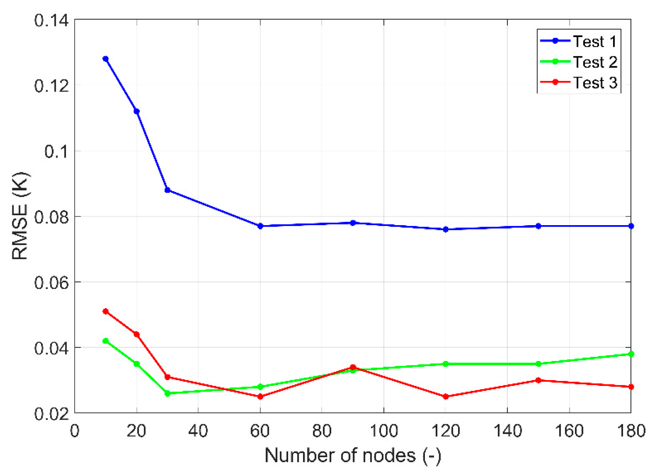
Eight different simulation cases with a number of nodes equal to 10, 20, 30, 60, 90, 120, 150, and 180 nodes, respectively, were compared to three different charging experiments. The Root Mean Square Error (RMSE) was estimated, as shown in Equation (1), by comparing each temperature simulation result for the five different ports at the time the test’s completion setpoint is reached with the experimental results for all three experiments. The RMSE results for each number of nodes tested and for the three tests are presented in Figure 8. As can be observed, for a number of nodes higher than 60, the improvement is relatively small. In fact, this comes in agreement with the study by Wischhusen [53], which mentions that for a relatively low number of nodes (n < 20), the buoyancy effects harm the accuracy of the model [54]. Hence, to minimize, as much as possible, the calculation time, the number of nodes used in the following tests was set equal to 60. The final model parameters are reported in

Table A4. Simulation Parameters of Type340 used for the combi-storage model.

Property	Value	Unit
Storage Height	1.61	m
Storage Volume	0.535	m3
Specific Heat	4.18	kJ/kgK
Density	998	kg/m3
Effective thermal conductivity	2.2	kJ/h/m/K
Initial Temp	20	°C
UA loss capacity rate on the bottom	5.97	kJ/h/K
UA loss capacity rate at the top	0.24	kJ/h/K
Relative length of the heat loss zone 1	1	-
UA loss capacity rate for heat loss 1	4.6	kJ/h/K
Rel. Position double port #1—Inlet	0.082	-
Rel. Position double port #1—Outlet	0.918	-
Stratified Charging for double port #1	No	-
Rel. Position double port #2—Inlet	0.708	-
Rel. Position double port #2—Outlet	0.500	-
Stratified Charging for double port #2	No	-
Rel. Position double port #3—Inlet (same as double port #1 inlet)	0.082	-
Rel. Position double port #3—Outlet	0.29	-
Stratified Charging for double port #3	No	-
Rel. position of Sensor #1 (TCS1)	0.082	-
Rel. position of Sensor #2 (TCS2)	0.290	-
Rel. position of Sensor #3 (TCS3)	0.500	-
Rel. position of Sensor #4 (TCS4)	0.708	-
Rel. position of Sensor #5 (TCS5)	0.918	-
Heat exchangers	Not Used	-
Nr of Nodes	60	-

of the Appendix A.

$$RMSE=\sqrt{\frac{1}{N}\sum _{i=1}^{N=5}{\left({\theta }_{pred,i}-{\theta }_{meas,i}\right)}^2}$$

(1)

3.2. DHW Demand Profile Sensitivity Analysis

As already stated in the previous section, the DHW profile was modeled based on the Type 14 “forcing function water draw”. In order to model the profile, the daily interval is divided into 96 equal periods. The DHW demand is assumed to be generated at the beginning of each period.

For the test rig’s case, under a constant flowrate of 0.18 L/s and with a temperature rise of 25 K, the equivalent liters of hot water, corresponding to an energy consumption of 5.845 kWh (Table A1), were equal to 200.4 L. In order to compare the model’s DHW profile area over a 24-h period with the aforementioned target volume, a quantity integrator (Type 24) connected with a scope (Type 76) was used.

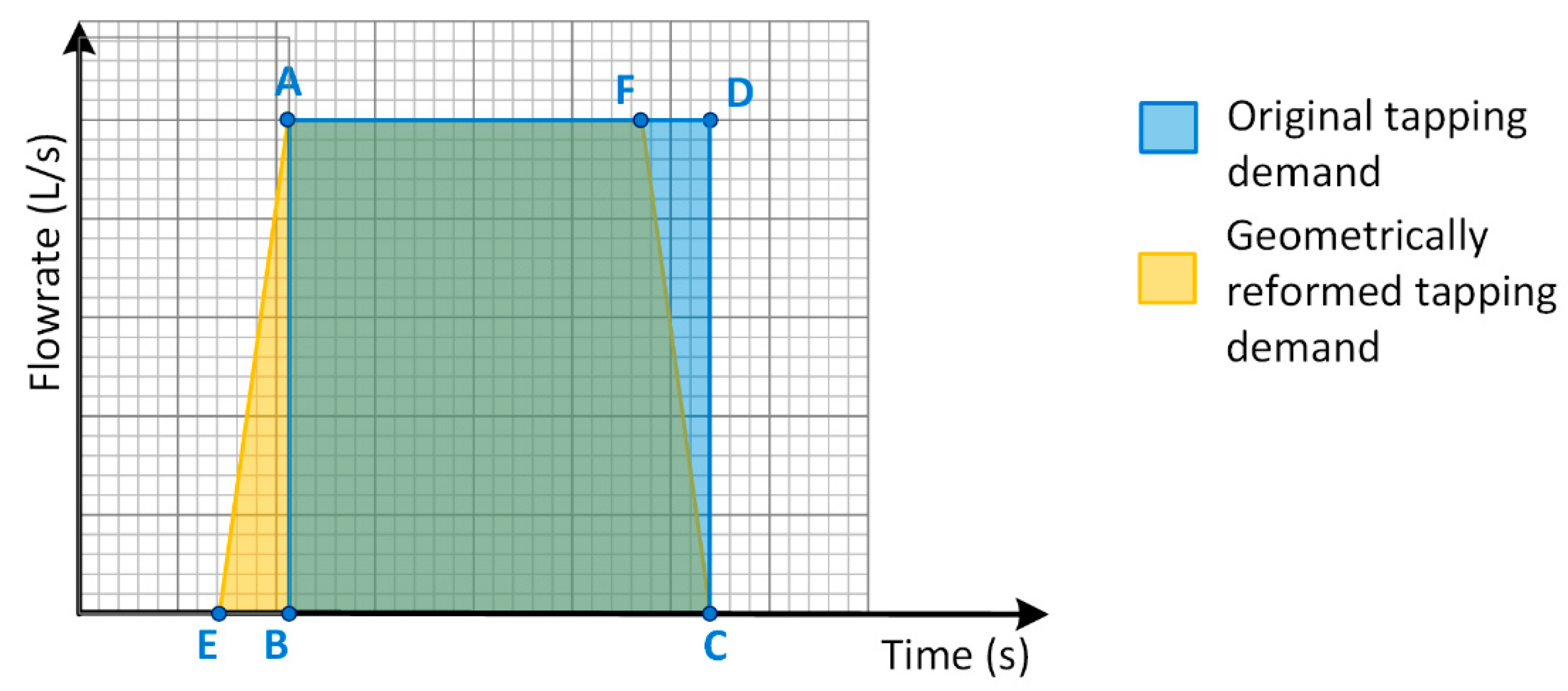
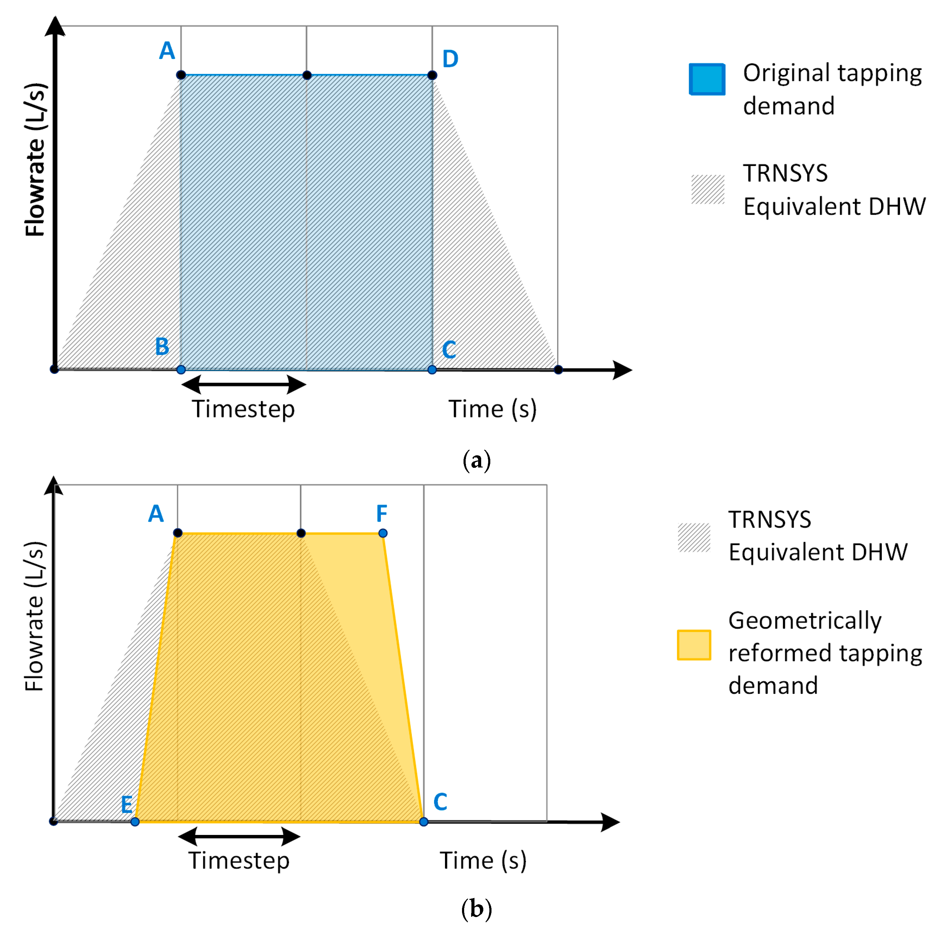
When a timestep of 60 s was used, an absolute difference of 145.2 L was observed (the absolute difference between the estimated volume by TRNSYS and the equivalent volume of 200.4 L). This large deviation is owed to the calculation approach of the DHW profile by the TRNSYS algorithm. In fact, the algorithm calculates the value of the forcing function at the beginning and ending of the time step, joining the two points via a line. Hence, the rectangular area of the forcing function is transformed into a trapezoid, leading to an overshooting of energy consumption. In order to overcome this deviation, two approaches could be applied:

• Decreasing the time step at the expense of a larger computational cost.
• Geometrical reforming of the function. The reforming is realized by starting the forcing function rise by a specific time constant earlier than the actual tapping event time and starting the decline curve earlier, with the same time constant as before, prior to the calculated tapping duration. In order to visualize the applied method, Figure 9 presents the geometrical reforming of the step function. Considering the original tapping demand to be depicted by the rectangular ABCD, the proposed reforming is represented by the trapezoid AECF. More specifically, the tapping demand is considered to start at an earlier time, equal to (EB). In accordance with the earlier start of the tapping and in order to circulate an equal amount of liters, the tapping starts to decrease at a time duration equal to (EB), earlier than the original demand, eventually leading to the formation of the reformed trapezoid. By applying this method, the user is able to control the TRNSYS calculation algorithm of the forcing function and thus minimize the calculation error for a given time step.

In order to make clearer the impact of the geometrical reforming in the correction of the estimated equivalent DHW volume, a qualitative example of the estimation derived from the original rectangular-shaped tapping demand and the corresponding estimation by the geometrical reforming are shown in Figure 10a,b, respectively.

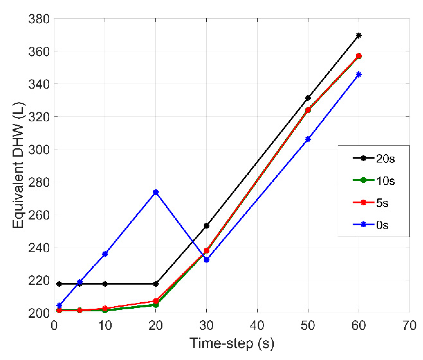
Based on the above, the time duration (EB) and the time step used in the DHW profile need to be determined to minimize the error with the trapezoid reforming. Hence, a dedicated sensitivity analysis was conducted. Four different (EB) duration values were evaluated, namely 0 s, 5 s, 10 s, and 20 s. By applying the four different durations under seven different time steps (1, 5, 10, 20, 30, 50, and 60 s), the results presented in Figure 11 were obtained. 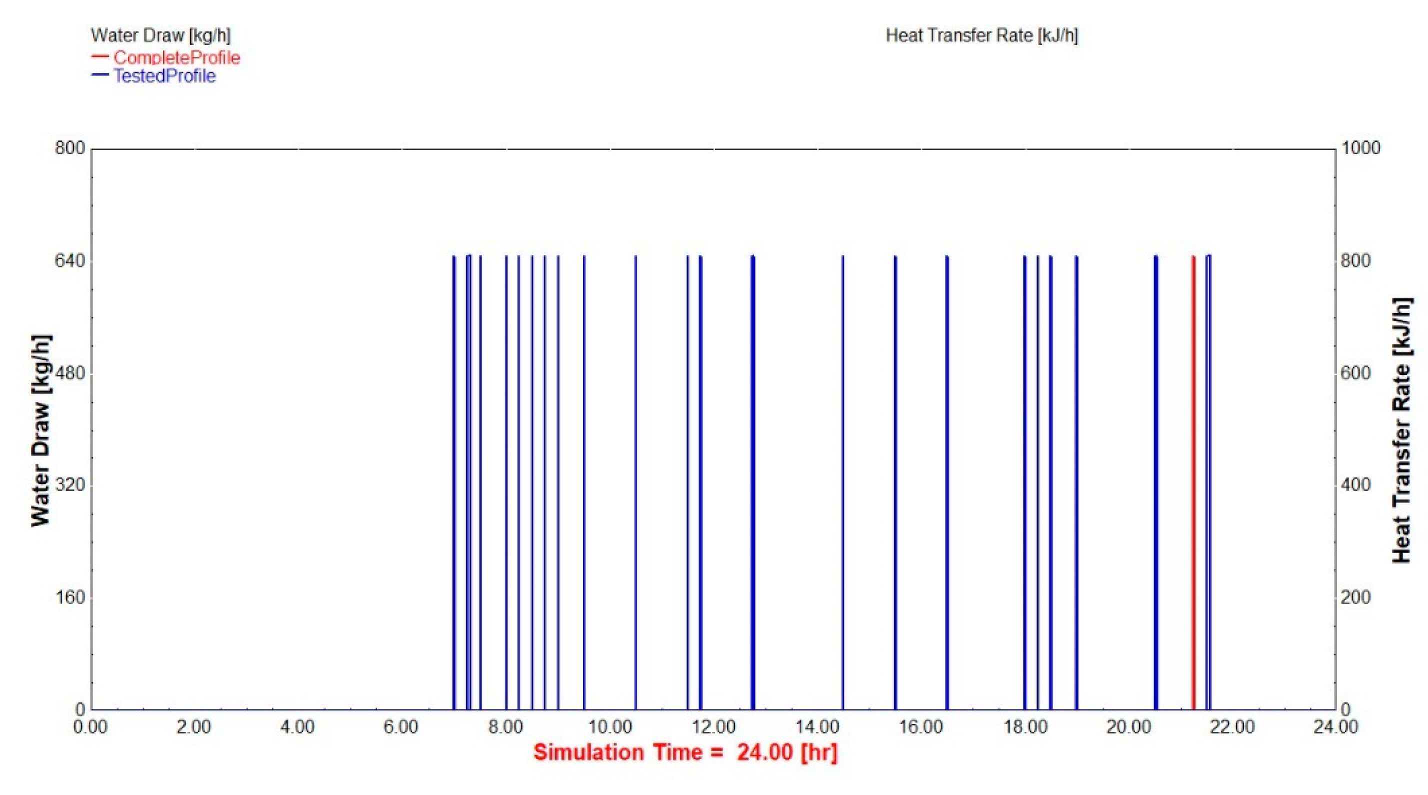As can be seen in Figure 11, the optimal results were obtained for a time duration (EB) of 10 s, while for all the rest of the time durations, smaller time steps enhanced the calculation deviation. On the other hand, for time steps larger than 30 s, the smaller deviation was recorded for a time duration of 0 s (i.e., without reforming). However, this is attributed to the fact that an entire tapping use (at around 21:15) failed to be calculated. In order to prove this conclusion, the water draw profile of

Table A3. Equivalent daily demand profile for DHW.

No. of Consumption	Start (hh:mm)	Duration of Consumption for 18.81 kW (s)	No. of equivalent CONSUMPTION	Duration of Equivalent Consumption (s)
1	07:00	20.09
2	07:17	267.94
3	07:30	20.09	1	308.13
4	08:00	20.09
5	08:15	20.09
6	08:30	20.09
7	08:45	20.09
8	09:00	20.09
9	09:30	20.09	2	120.57
10	10:30	20.09
11	11:30	20.09
12	11:45	20.09	3	60.29
13	12:45	60.28	4	60.28
14	14:30	20.09
15	15:30	20.09
16	16:30	20.09	5	60.29
17	18:00	20.09
18	18:15	20.09
19	18:30	20.09
20	19:00	20.09	6	80.38
21	20:30	140.67
22	21:15	20.09	7	140.67
23	21:30	267.94	8	288.04

was used as an input scenario for a timestep of 30 s and for EB = 0, as depicted in the dedicated run of Figure 12 (denoting with red the missed tapping). Regarding the time step for a specific time duration, time steps of equal or lower value than the time duration result in a constant result. On the contrary, for larger time steps, the result is unstable.

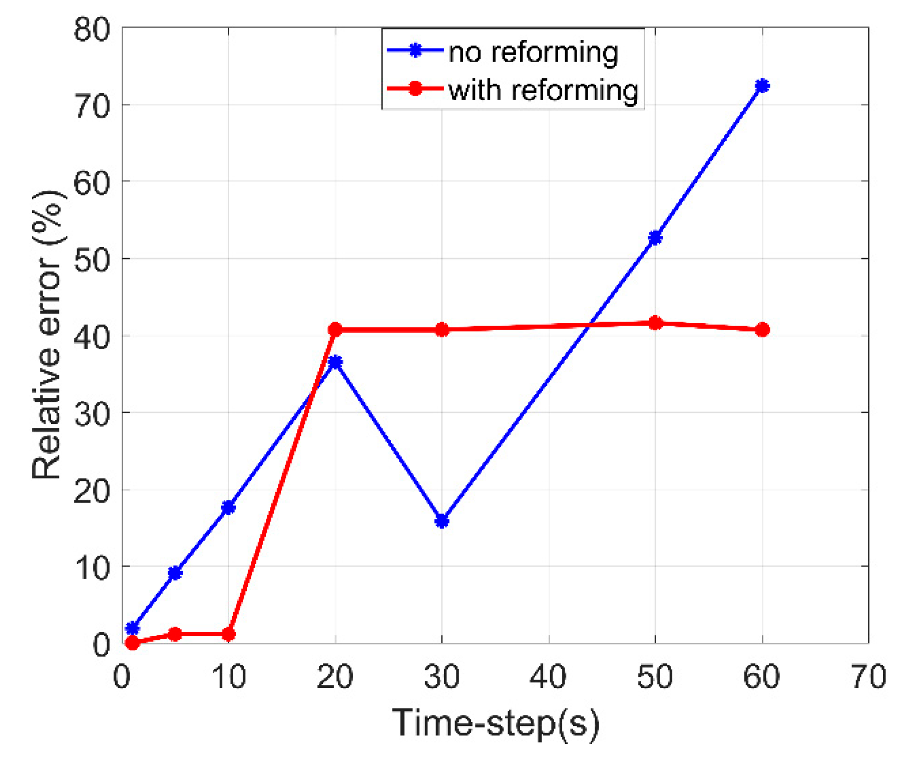
However, using the trapezoid reforming, the time period during which the demand is non-zero is larger than the time period (BC). In order to bypass this setback, the EA linear fraction is shifted parallelly until E==B. A second sensitivity analysis was conducted with the adapted trapezoid under the same time-step scenarios as in Figure 11. In this sensitivity analysis, the time duration EB was considered under four scenarios: 0 s, 1 s, 5 s, and 10 s. The control signal of the DHWP was multiplied by the pump’s constant flowrate, and the result was integrated over a single-day period. The results are depicted in

Table 4. Sensitivity analysis for hot water supplied by DHWP in a single day.

	Hot Water Daily Supply (L)
Time Step (s)	(EB) = 0 s	(EB) = 1 s	(EB) = 5 s	(EB) = 10 s
60	345.6	118.8	118.8	118.8
50	306.0	117	117	117
30	232.2	118.8	118.8	118.8
20	273.6	118.8	118.8	118.8
10	235.8	198	198	198
5	218.7	198	198	198
1	204.3	200.5	200.5	200.5

. As shown, the accuracy of the results is heavily influenced by the time step and the use of the reforming, while it is not affected by the time duration (EB). This conclusion can be more easily visualized in Figure 13, where the relative error with and without the application of geometrical reforming is shown. Based on the above results, a value of 10 s was selected as the optimal time duration (EB), while the time step was selected to be 10 s as well, in order to minimize the computational time. These settings were applied in all the case studies presented in the next section.

3.3. Charging of Entire Tank

Within the context of the combi-storage tank use for DHW and space heating, four additional experiments were conducted and are presented in the following three subsections. The reason for these experiments was twofold: the further validation of the simulation model and the experimental assessment of the proposed combi-storage tank for use in residential space heating and DHW applications.

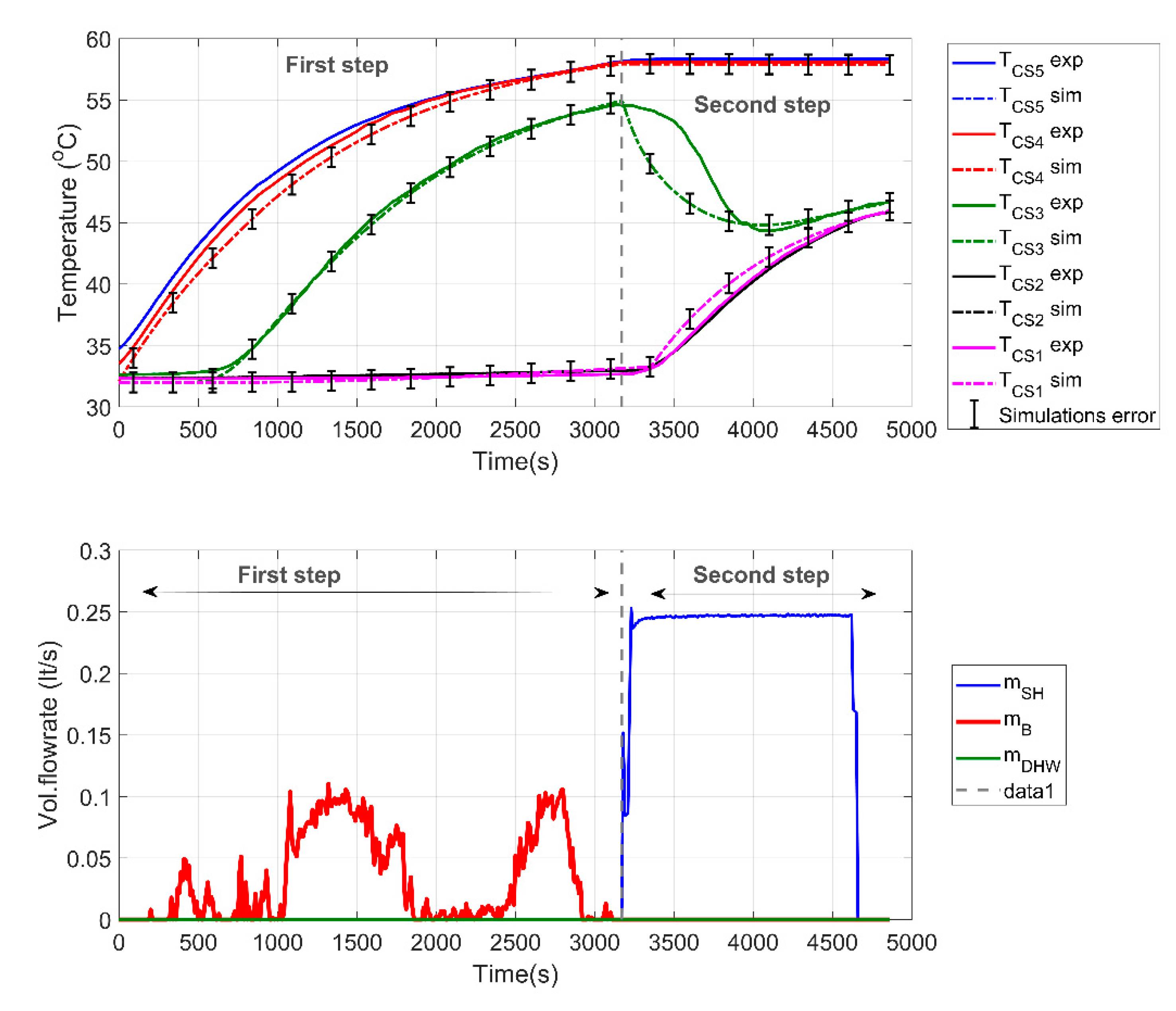
The first experiment involved the charging of both sections of the tank in two subsequent steps, as shown in Figure 14. In the first step (from 0s up to 3170 s), the upper part of the tank was charged via port 4 (Figure 2). The flowrate of the HWBP was set at 0.14 L/s, while the gas boiler setpoint was equal to 60 °C. The initial conditions in the combi-tank included a uniform temperature of approximately 36 °C, and the target values were 58 °C for the temperatures $T_{CS4}$ and $T_{CS5}$. In the second step of the test (from 3170 s up to the end), after the upper part was charged, the lower part of the tank, dedicated to covering the space heating loads, was also heated via port 1 with a flow rate of 0.25 L/s. The respective boiler setpoint was set at a water temperature of 50 °C.

As shown in Figure 14, in the first step of the charging process, there is a good agreement between the experimental and the simulation results after approximately 1800 s. By that time, all five experimentally measured temperatures fall within the range of the estimated values by the simulations, for considered errors of ±0.6 °C. As the heat is introduced in the tank via port 4, temperatures, $T_{CS4}$ and $T_{CS5}$. rise from the start in a close range, while $T_{CS3}$ has a delayed increase in the temperature. Finally, $T_{CS1}$ and $T_{CS2}$ are practically not influenced throughout this step, revealing a good stratification behavior of the tank. Once the second step is initiated, and heat is fed via the tank’s lower port (port 1),$T_{CS1}$ and $T_{CS2}$ show a sharp rise; on the other hand, $T_{CS3}$ is also influenced, tending to mix with the lower parts of the tank and therefore reducing its temperature. The stepwise change in the flowrates results in a deviation between the model and the experiments, in particular for $T_{CS3}$, which re-converges after approximately 1000 s. Finally, $T_{CS4}$ and $T_{CS5}$. tend to be unaffected by the space heating charging, a behavior that comes in agreement with both experimental and simulation results.

3.4. Space Heating Test

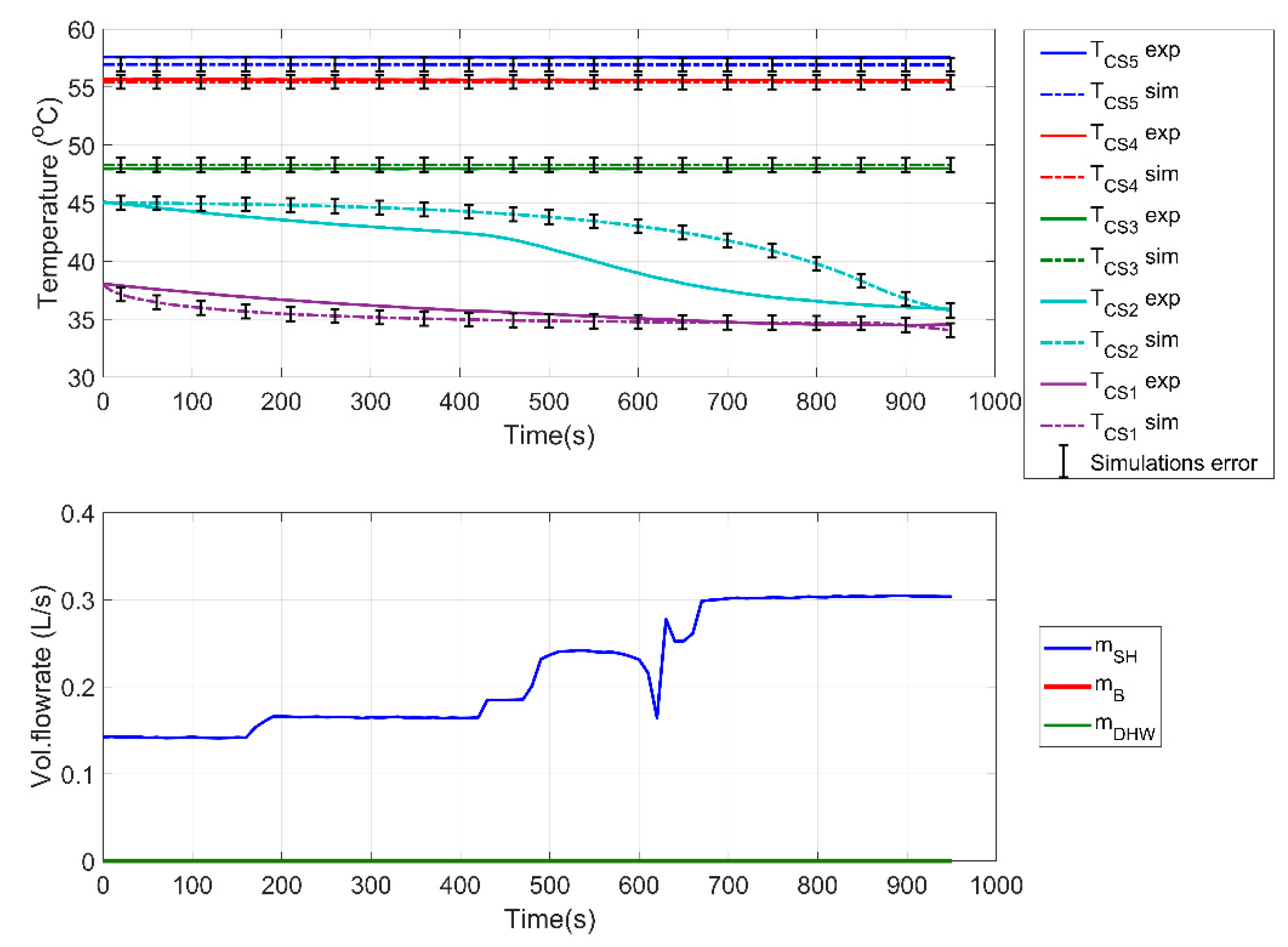
The next set of experiments aimed at testing the space heating performance of the experimental system and the simulation model, respectively. The supply flow rate for this experiment was equal to 0.14 L/s, corresponding to a temperature difference equal to 10 °C (considering a supply temperature from the tank of 43 °C and a return temperature of 33 °C). The total thermal power corresponded to approximately 6 kW. This power supply to the heating system was estimated to be the maximum thermal power needed, based on typical nZEB building simulations [46,55]. When space heating is supplied exclusively from the combi-storage tank, the space heating supply temperature to the heat exchanger (Figure 2) is regulated by a mixing valve, so that the inlet to the hypothetical floor heating system is kept at 38 °C. As can be observed by the results of Figure 15, although the model accurately predicts the final temperature profiles of the tank, there are some deviations occurring due to the lack of detailed inertia modeling of both the tank and the rest of the system components. This is especially evident as far as $T_{CS2}$ is concerned, which is influenced the most by inertia phenomena, as was also observed in the experimental data. In this scenario, $T_{CS2}$ shows a stronger trend to mix with the lower section of the tank compared to the simulation. Thus, the simulation model presents a slightly better stratification behavior than the experimental procedure actually revealed.

3.5. DHW Test

In order for the DHW tests to be conducted, the combi-storage tank is priorly fully charged ($T_{CS4}$ and $T_{CS5}$ equal to 58 °C). The first test conducted with respect to DHW investigated the maximum power (worst case) scenario, which corresponded to the largest power consumption of the used water profile (as mentioned in Section 2.4, load profiles for cycle no. 2 of the European Standard [41] were used). Hence, an 18.81 kW load was considered for a total duration of 18.65 min, which corresponds to the total consumed energy of 5.85 kWh. The boiler was turned on when $<$55.5 °C, with a nominal DHW flowrate of 0.3 L/s and a ΔΤ equal to 15 Κ. The above selection in the ΔΤ and the corresponding flowrate were partially dictated by the available cold-water supply in Athens, Greece, during the time of the experiments (July 2020) and were equal to approximately 27 °C. The nominal supply and return temperatures were set equal to 58 °C and 33 °C, respectively.

As seen in Figure 16, the used working conditions maintained the temperatures $T_{CS1}$ and $T_{CS2}$ above 42 °C during the experiment, despite the low temperature return of the DHW consumption. However, in the upper part of the tank, temperatures decreased rapidly, resulting in the need for additional heat input after 490 s. With respect to the simulation model results, as shown in Figure 16, the rapid temperature changes, in particular, $T_{CS4}$ and $T_{CS5}$, were not accurately predicted by the model, which required approximately 1000 s and close to steady state conditions in order to converge at an acceptable level. These results highlight that such storage tank models can be used for steady-state (on-/off-design) simulations, which in particular for solar-driven systems commonly have hourly or larger timesteps but should be avoided for dynamic and semi-dynamic simulations as they tend to deviate considerably.

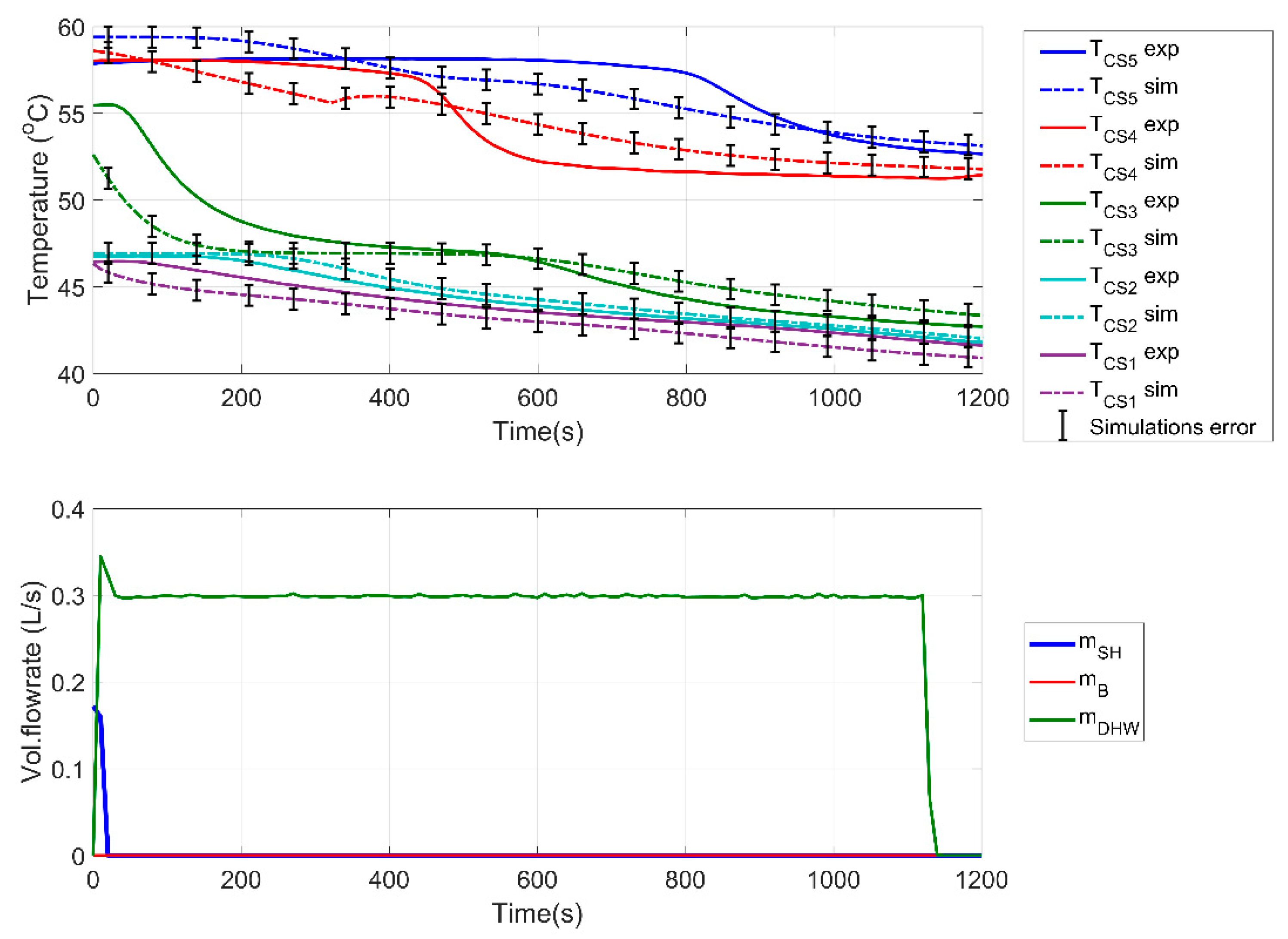
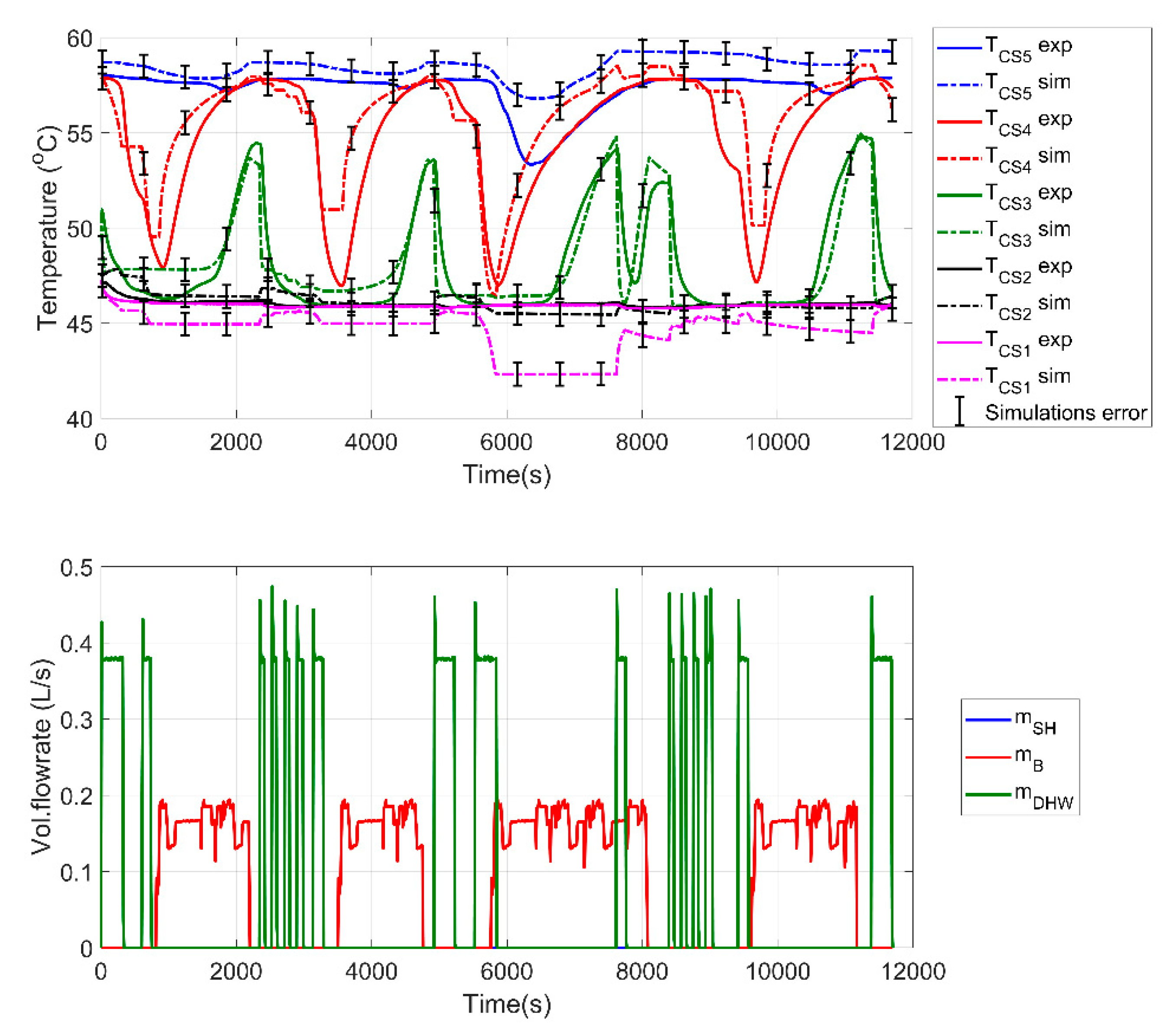
In order to find a suitable switch-on temperature criterion for the boiler that minimizes the number of cut-off/switch-on cycles while ensuring a reliable supply temperature for SH and DHW, the combi-storage tank’s behavior was further investigated by conducting a second DHW test. In this case, a combination of both $T_{CS4}$ and $T_{CS5}$ ($\frac{T_{CS4}+T_{CS5}}{2}$ < 53 °C) was introduced in the control criteria in order to be able to deal with the temperature drop due to DHW consumption and provide hot water at acceptable temperature levels. Moreover, two alternative criteria were set for the boiler to be turned on in order to deal with the temperature drop due to heat losses and internal mixing ($T_{CS4}$ < 50 °C or $T_{CS5}$ < 56 °C). Eventually, the boiler was turned on in case any of the aforementioned three criteria were not satisfied. The boiler was then turned off again when $T_{CS5}$ was heated above 58 °C.

For the purposes of this experiment, an equivalent profile was created by grouping the original DHW profile of the European standard’s consumptions into eight different groups, as presented in Table A3 of the Appendix A. Two complete cycles were executed in the experiment to ensure that the performance of the tank was adequate, even if it was partially discharged at the beginning of the cycle.

The results of this experiment are presented in Figure 17 along with the respective simulation model results. The used criteria are considered to be adequate, as $T_{CS5}$ remains well above 50 °C in all cases, which is an acceptable scenario for DHW use. However, as can be observed, the boiler is needed to operate with relatively high temperature input and for small ΔΤ (minimum $T_{CS4}$ was 47.1 °C and minimum $T_{CS3}$ was 45.9 °C), not allowing the condensation to take place and thus dramatically decreasing the boiler’s efficiency. With respect to the simulation model, similarly to the previous cases, the transient states are not adequately predicted by the model, with the temperatures of the upper levels of the tank being constantly over-predicted and the lower levels’ temperatures being under-predicted. This longer experiment, with more fluctuations, highlights again the incompatibility of the model for transient simulations. However, it has to be noted that in cases where transient phenomena are not of concern and the time-step of the simulations is larger, the model can adequately predict the storage’s behavior since, as shown in Figure 17, eventually the temperature profiles converge to the temperatures measured during the experiments.

4. Conclusions

In this study, the experiments conducted in a combi-storage tank test rig used to cover the space heating and DHW needs of a nZEB building were analyzed. A dedicated simulation model was developed in TRNSYS software and tested in comparison to the experimental data. The main conclusions of the analysis can be summarized below:

• Based on the case study and the specifications of the storage tank, there are a number of nodes for the simulation model discretization, beyond which the benefits to the model’s accuracy are negligible. In this study, this threshold was found to be 60 nodes.
• In the charging test of the upper part of the tank, there was a good stratification profile in the tank, which was also predicted sufficiently by the model. However, once the charging of the lower parts of the tank started, the deviation of the model from the experiments increased and required a sufficient amount of time to reconverge, revealing the inadequacy of the model to predict transient phenomena.
• A similar behavior was obtained during the heating tests, as the lack of detailed inertia modeling of both the tank and the rest of the system components resulted in deviations during transient conditions, despite accurately predicting the final temperature profiles of the tank. Moreover, the aforementioned deviations resulted in the simulation model presenting a slightly better stratification behavior than the one actually measured during the experiments.
• With respect to DHW tests, a multi-criteria approach was introduced to successfully control the operation of the gas boiler and ensure an acceptable performance of the combi-storage tank under the considered DHW loads. In fact, the upper temperature of the tank was kept in all cases above 50 °C, with time margins indicating that the boiler was needed to heat up the lower parts of the tank. On the other hand, the simulation model failed to predict the transient states of the tank, while the final levels of temperature were well predicted at all five points of measurement in the tank.
• Eventually, the 1D simulation model developed and tested in this study will be adequate for use in on- and off-design models where transient phenomena are not of importance, while for dynamic and semi-dynamic simulations, more detailed models should be preferred.

References

1. Pallis, P.; Gkonis, N.; Varvagiannis, E.; Braimakis, K.; Karellas, S.; Katsaros, M.; Vourliotis, P. Cost effectiveness assessment and beyond: A study on energy efficiency interventions in Greek residential building stock. Energy Build. 2019, 182, 1–18. [Google Scholar] [CrossRef]
2. European Union. DIRECTIVE (EU) 2018/2001 of The European Parliament and of The Council 328/82; European Union: Brussels, Belgium, 2018. [Google Scholar]
3. Roumpedakis, T.C.; Kallis, G.; Magiri-Skouloudi, D.; Grimekis, D.; Karellas, S. Life cycle analysis of ZEOSOL solar cooling and heating system. Renew. Energy 2020, 154, 82–98. [Google Scholar] [CrossRef]
4. Yaïci, W.; Entchev, E. Performance prediction of a solar thermal energy system using artificial neural networks. Appl. Therm. Eng. 2014, 73, 1348–1359. [Google Scholar] [CrossRef]
5. Eurostat. Εnergy Consumption in Households. Available online: https://ec.europa.eu/eurostat/statistics-explained/index.php?title=Energy_consumption_in_households#Energy_products_used_in_the_residential_sector (accessed on 1 May 2023).
6. Garg, H.; Mullick, S.; Bhargava, V.K. Solar Thermal Energy Storage; Springer Science & Business Media: Berlin/Heidelberg, Germany, 2012. [Google Scholar]
7. Sarbu, I.; Sebarchievici, C. A Comprehensive Review of Thermal Energy Storage. Sustainability 2018, 10, 191. [Google Scholar] [CrossRef]
8. Raccanello, J.; Rech, S.; Lazzaretto, A. Simplified dynamic modeling of single-tank thermal energy storage systems. Energy 2019, 182, 1154–1172. [Google Scholar] [CrossRef]
9. Salomoni, V.A.; Majorana, C.E.; Giannuzzi, G.M.; Miliozzi, A.; Di Maggio, R.; Girardi, F.; Mele, D.; Lucentini, M. Thermal storage of sensible heat using concrete modules in solar power plants. Sol. Energy 2014, 103, 303–315. [Google Scholar] [CrossRef]
10. Karellas, S.; Roumpedakis, T.C. Chapter 7—Solar thermal power plants. In Solar Hydrogen Production; Calise, F., D’Accadia, M.D., Santarelli, M., Lanzini, A., Ferrero, D., Eds.; Academic Press: Cambridge, MA, USA, 2019; pp. 179–235. [Google Scholar]
11. Cabeza, L.F.; Martorell, I.; Miró, L.; Fernández, A.I.; Barreneche, C. 1—Introduction to thermal energy storage systems. In Advances in Thermal Energy Storage Systems, 2nd ed; Cabeza, L.F., Ed.; Woodhead Publishing: Cambridge, UK, 2021; pp. 1–33. [Google Scholar]
12. Palomba, V.; Frazzica, A. Recent advancements in sorption technology for solar thermal energy storage applications. Sol. Energy 2019, 192, 69–105. [Google Scholar] [CrossRef]
13. Abedin, A.H.; Rosen, M.A. A critical review of thermochemical energy storage systems. Open Renew. Energy J. 2011, 4, 42–46. [Google Scholar] [CrossRef]
14. Lahmidi, H.; Mauran, S.; Goetz, V. Definition, test and simulation of a thermochemical storage process adapted to solar thermal systems. Sol. Energy 2006, 80, 883–893. [Google Scholar] [CrossRef]
15. Morofsky, E. History of Thermal Energy Storage; Springer: Dordrecht, The Netherlands, 2007; pp. 3–22. [Google Scholar]
16. Ter-Gazarian, A. The Institution of Engineering and Technology. In Energy Storage for Power Systems; Academic Press: Cambridge, MA, USA, 2011. [Google Scholar]
17. Chidambaram, L.A.; Ramana, A.S.; Kamaraj, G.; Velraj, R. Review of solar cooling methods and thermal storage options. Renew. Sustain. Energy Rev. 2011, 15, 3220–3228. [Google Scholar] [CrossRef]
18. Alva, G.; Lin, Y.; Fang, G. An overview of thermal energy storage systems. Energy 2018, 144, 341–378. [Google Scholar] [CrossRef]
19. Gil, A.; Medrano, M.; Martorell, I.; Lázaro, A.; Dolado, P.; Zalba, B.; Cabeza, L.F. State of the art on high temperature thermal energy storage for power generation. Part 1—Concepts, materials and modellization. Renew. Sustain. Energy Rev. 2010, 14, 31–55. [Google Scholar] [CrossRef]
20. Tian, Y.; Zhao, C.Y. A review of solar collectors and thermal energy storage in solar thermal applications. Appl. Energy 2013, 104, 538–553. [Google Scholar] [CrossRef]
21. Hasan Ismaeel, H.; Yumrutaş, R. Investigation of a solar assisted heat pump wheat drying system with underground thermal energy storage tank. Sol. Energy 2020, 199, 538–551. [Google Scholar] [CrossRef]
22. Syed, A.; Izquierdo, M.; Rodríguez, P.; Maidment, G.; Missenden, J.; Lecuona, A.; Tozer, R. A novel experimental investigation of a solar cooling system in Madrid. Int. J. Refrig. 2005, 28, 859–871. [Google Scholar] [CrossRef]
23. Karim, A.; Burnett, A.; Fawzia, S. Investigation of Stratified Thermal Storage Tank Performance for Heating and Cooling Applications. Energies 2018, 11, 1049. [Google Scholar] [CrossRef]
24. Pintaldi, S.; Sethuvenkatraman, S.; White, S.; Rosengarten, G. Energetic evaluation of thermal energy storage options for high efficiency solar cooling systems. Appl. Energy 2017, 188, 160–177. [Google Scholar] [CrossRef]
25. Jung, W.; Kim, D.; Kang, B.H.; Chang, Y.S. Investigation of Heat Pump Operation Strategies with Thermal Storage in Heating Conditions. Energies 2017, 10, 2020. [Google Scholar] [CrossRef]
26. Çomaklı, K.; Çakır, U.; Kaya, M.; Bakirci, K. The relation of collector and storage tank size in solar heating systems. Energy Convers. Manag. 2012, 63, 112–117. [Google Scholar] [CrossRef]
27. Li, T.; Liu, Y.; Wang, D.; Shang, K.; Liu, J. Optimization Analysis on Storage Tank Volume in Solar Heating System. Procedia Eng. 2015, 121, 1356–1364. [Google Scholar] [CrossRef]
28. Pinel, P.; Cruickshank, C.A.; Beausoleil-Morrison, I.; Wills, A. A review of available methods for seasonal storage of solar thermal energy in residential applications. Renew. Sustain. Energy Rev. 2011, 15, 3341–3359. [Google Scholar] [CrossRef]
29. Schmidt, T.; Mangold, D. Conversion of Germany’s first seasonal solar thermal energy storage into an innovative multifunctional storage. In Proceedings of the EuroSun 2010: International Conference on Solar Heating, Cooling and Buildings, Graz, Austria, 28 September–1 October 2010. [Google Scholar]
30. Terziotti, L.T.; Sweet, M.L.; McLeskey, J.T. Modeling seasonal solar thermal energy storage in a large urban residential building using TRNSYS 16. Energy Build. 2012, 45, 28–31. [Google Scholar] [CrossRef]
31. Sweet, M.L.; McLeskey, J.T. Numerical simulation of underground Seasonal Solar Thermal Energy Storage (SSTES) for a single family dwelling using TRNSYS. Sol. Energy 2012, 86, 289–300. [Google Scholar] [CrossRef]
32. Antoniadis, C.N.; Martinopoulos, G. Simulation of Solar Thermal Systems with Seasonal Storage Operation for Residential Scale Applications. Procedia Environ. Sci. 2017, 38, 405–412. [Google Scholar] [CrossRef]
33. Hailu, G.; Hayes, P.; Masteller, M. Long-Term Monitoring of Sensible Thermal Storage in an Extremely Cold Region. Energies 2019, 12, 1821. [Google Scholar] [CrossRef]
34. Hesaraki, A.; Holmberg, S.; Haghighat, F. Seasonal thermal energy storage with heat pumps and low temperatures in building projects—A comparative review. Renew. Sustain. Energy Rev. 2015, 43, 1199–1213. [Google Scholar] [CrossRef]
35. Li, H.; Sun, L.; Zhang, Y. Performance investigation of a combined solar thermal heat pump heating system. Appl. Therm. Eng. 2014, 71, 460–468. [Google Scholar] [CrossRef]
36. Drosou, V.N.; Tsekouras, P.D.; Oikonomou, T.I.; Kosmopoulos, P.I.; Karytsas, C.S. The HIGH-COMBI project: High solar fraction heating and cooling systems with combination of innovative components and methods. Renew. Sustain. Energy Rev. 2014, 29, 463–472. [Google Scholar] [CrossRef]
37. Gabrielli, P.; Gazzani, M.; Martelli, E.; Mazzotti, M. Optimal design of multi-energy systems with seasonal storage. Appl. Energy 2018, 219, 408–424. [Google Scholar] [CrossRef]
38. McKenna, R.; Fehrenbach, D.; Merkel, E. The role of seasonal thermal energy storage in increasing renewable heating shares: A techno-economic analysis for a typical residential district. Energy Build. 2019, 187, 38–49. [Google Scholar] [CrossRef]
39. Klein, S.A.; Beckman, W.A.; Mitchell, J.W.; Duffie, J.A.; Duffie, N.A.; Freeman, T.L. TRNSYS 18: A Transient System Simulation Program; Solar Energy Laboratory, University of Wisconsin: Madison, WI, USA, 2017. [Google Scholar]
40. Kumar, K.; Singh, S. Investigating thermal stratification in a vertical hot water storage tank under multiple transient operations. Energy Rep. 2021, 7, 7186–7199. [Google Scholar] [CrossRef]
41. European Committee for Standardization (CEN). EN 13203-2:2018 Gas-Fired Domestic Appliances Producing Hot Water Part 2: Assessment of Energy Consumption; European Committee for Standardization: Brussels, Belgium, 2018. [Google Scholar]
42. D’agostino, D.; Zangheri, P.; Castellazzi, L. Towards nearly zero energy buildings in Europe: A focus on retrofit in non-residential buildings. Energies 2017, 10, 117. [Google Scholar] [CrossRef]
43. Attia, S. Chapter 1—Introduction to NZEB and Market Accelerators. In Net Zero Energy Buildings (NZEB); Attia, S., Ed.; Butterworth-Heinemann: Oxford, UK, 2018; pp. 1–20. [Google Scholar]
44. Che, D.; Liu, Y.; Gao, C. Evaluation of retrofitting a conventional natural gas fired boiler into a condensing boiler. Energy Convers. Manag. 2004, 45, 3251–3266. [Google Scholar] [CrossRef]
45. ©RIELLO SPA. RESIDENCE. CONDENSING WALL HUNG BOILERS—RESIDENCE 25 KIS. Available online: https://www.riello.com/international/products/heating-catalogue-products/residence_R-EX-PL-0011659?k=Product+Line%7CR-EX-PL-0004110%7C- (accessed on 20 June 2023).
46. Pallis, P.; Gkonis, N.; Varvagiannis, E.; Braimakis, K.; Karellas, S.; Katsaros, M.; Vourliotis, P.; Sarafianos, D. Towards NZEB in Greece: A comparative study between cost optimality and energy efficiency for newly constructed residential buildings. Energy Build. 2019, 198, 115–137. [Google Scholar] [CrossRef]
47. Thornton, J.; Bradley, D.; McDowell, T.; Blair, N.; Duffy, M.; LaHam, N.; Naik, A. TESSLibs 17-Component Libraries for the TRNSYS Simulation Environment Volume 11 Storage Tank Library Mathematical Reference. Tesscomponent Libr. 2012, 11, 1–93. [Google Scholar]
48. Remund, J.; Müller, S.; Schmutz, M.; Graf, P. Meteonorm Version 8. Available online: www.meteotest.com (accessed on 14 September 2023).
49. Drück, H. Multiport Store Model for TRNSYS-Stratified Fluid Storage Tank with four Internal Heat Exchangers. In Ten Connections for Direct Charge and Discharge and an Internal Electrical Heater (type340); University of Stuttgart: Stuttgart, Germany, 2006. [Google Scholar]
50. Su, Z.; Yang, L. Peak shaving strategy for renewable hybrid system driven by solar and radiative cooling integrating carbon capture and sewage treatment. Renew. Energy 2022, 197, 1115–1132. [Google Scholar] [CrossRef]
51. Allard, Y.; Kummert, M.; Bernier, M. Intermodel comparison and experimental validation of electrical water heater models in TRNSYS. In Proceedings of the Building Simulation 2011, Sydney, NSW, Australia, 14–16 November 2011; pp. 688–695. [Google Scholar]
52. Manouchehri, R.; Collins, M.R. Investigating the Impact of Plumbing Configuration on Energy Savings for Falling-Film Drain Water Heat Recovery Systems. Energies 2022, 15, 1141. [Google Scholar] [CrossRef]
53. Wischhusen, S. An enhanced discretization method for storage tank models within energy systems. In Proceedings of the 5th International Modelica Conference, Vienna, Austria, 4–5 September 2006; pp. 243–248. [Google Scholar]
54. Roumpedakis, T.C.; Fostieris, N.; Braimakis, K.; Monokrousou, E.; Charalampidis, A.; Karellas, S. Techno-Economic Optimization of Medium Temperature Solar-Driven Subcritical Organic Rankine Cycle. Thermo 2021, 1, 77–105. [Google Scholar] [CrossRef]
55. Frazzica, A.; Brancato, V.; Dawoud, B. Unified Methodology to Identify the Potential Application of Seasonal Sorption Storage Technology. Energies 2020, 13, 1037. [Google Scholar] [CrossRef]
Figure 1. Schematic of the considered system. Different colors denote the various loops of the system at different temperature levels: Solar loop (Orange), STES charging (Brown), Solar charging of the Combi-storage tank (Red), Space Heating (Green), DHW (Grey), and Boiler charging the CST for DHW (Light Blue).
Thermo 03 00038 g001
Figure 2. Schematic of the experimental test rig. Different colors denote the various loops of the system at different temperature levels: (a) Domestic Hot Water loop (Orange); (b) Space heating loop (Blue) (c) Charging of the tank’s upper part (Red).
Thermo 03 00038 g002
Figure 3. Images of the experimental test rig configuration: Combi-storage tank (a), gas boiler, heat exchangers, and valves (b).
Thermo 03 00038 g003
Figure 4. Schematic of a combi-storage tank.
Thermo 03 00038 g004
Figure 5. (a) Piping drawing and (b) 3-D sketch of the piping geometry of the Combi-storage tank.
Thermo 03 00038 g005
Figure 6. Overview of the combi-storage tank TRNSYS model.
Thermo 03 00038 g006
Figure 7. Overview of the simplified nodes’ testing model of the combi-storage tank in TRNSYS.
Thermo 03 00038 g007
Figure 8. Overview of the statistical comparison of the tank model with experimental data for the various numbers of nodes.
Thermo 03 00038 g008
Figure 9. Proposed geometrical reforming for applying the step-function.
Thermo 03 00038 g009
Figure 10. A qualitative example of an equivalent DHW calculation for a given timestep for (a) original tapping demand and (b) geometrically reformed tapping demand.
Thermo 03 00038 g010
Figure 11. Timestep and geometrical reforming sensitivity analysis.
Thermo 03 00038 g011
Figure 12. Comparison of the complete water draw profile with the profile for EB = 0 and a timestep of 30 s.
Thermo 03 00038 g012
Figure 13. Relative error for the hot water supplied by DHWP per day for an (EB) time duration of 10 s.
Thermo 03 00038 g013
Figure 14. Full charging case study of the combi-storage tank.
Thermo 03 00038 g014
Figure 15. Heating case study of the combi-storage tank.
Thermo 03 00038 g015
Figure 16. DHW single consumption equals a daily energy demand.
Thermo 03 00038 g016
Figure 17. Equivalent DHW profile testing over a 2-day period is required.
Thermo 03 00038 g017