Article

Calculation Method for Traffic Load-Induced Permanent Deformation in Soils under Flexible Pavements

by
Mate Janos Vamos
1,2,* and
Janos Szendefy
2
1
CDM Smith SE, Darmstädter Str. 63, 64404 Bickenbach, Germany
2
Department of Engineering Geology and Geotechnics, Budapest University of Technology and Economics, Műegyetem rkp. 3, H-1111 Budapest, Hungary
*
Author to whom correspondence should be addressed.
Geotechnics 2023, 3(3), 955-974; https://doi.org/10.3390/geotechnics3030051
Submission received: 8 August 2023 / Revised: 30 August 2023 / Accepted: 14 September 2023 / Published: 21 September 2023
(This article belongs to the Topic Support Theory and Technology of Geotechnical Engineering)

Abstract

:
Rutting is one of the most common types of distress in flexible pavement structures. There are two fundamental methods of designing pavement structures: conventional empirical methods and analytical approaches. Many analytical and empirical design procedures assume that rutting is mostly of asphalt origin and can be reduced by limiting the vertical deformation or stress at the top of the subgrade, but they do not quantify the rutting depth itself. Mechanistic–empirical models to predict the permanent deformations of unbound pavement layers have been well investigated and are rather common in North America; however, they are not widely utilized in the rest of the world. To date, there is no generally accepted, widely recognized, and documented procedure for calculating permanent deformations and thus for determining the rutting depth in flexible pavement courses originating from the unbound granular layers. This paper presents a layered calculation method with which the deformation of soil layers (base, subbase, and subgrade courses) under flexible pavements due to repeated traffic load can be determined. In the first step, the cyclic strain amplitude is calculated using a nonlinear material model that is based on particle size distribution parameters (d50 and CU) and dependent on the mean normal stress, relative density, and actual strain level. In the second step, the HCA (High Cycle Accumulation) model is used to calculate the residual settlement of each sublayer as a function of the number of cycles. It is shown that the developed model is suitable for describing different types of subgrades and pavement cross-sections. It is also demonstrated with finite element calculations that the developed model describes both the elastic and plastic strains sufficiently accurately. The developed model can predict the settlement and rutting of pavement structures with sufficient accuracy based on easily available particle size distribution parameters without the need for complex laboratory and finite element tests.

1. Introduction

In flexible pavement structures, ruts can be also formed besides flexural and fatigue cracks, which can be caused by inadequate asphalt mixture, improperly compacted asphalt, or subsequent compaction of the soil caused by traffic. Conventional design procedures [1,2] do not consider permanent deformations from the compaction of the soil under traffic loads, and rutting is prevented by an appropriately chosen asphalt mixture and its careful compaction on site. Some analytical design procedures [3,4] assume that rutting is of soil origin only, and can be reduced by limiting the vertical deformation at the top of the subgrade, but does not quantify the rutting depth. In his Ph.D. thesis, Ref. [5] concluded based on in situ measurements that permanent settlements may not only be of soil origin, but the unbound granular base course can also significantly contribute to the rutting depending on the thickness of the asphalt course. Refs. [6,7,8] developed calculation procedures for the permanent deformation of unbound granular materials under repeated traffic loads.
There is no generally accepted, widely recognized, and documented procedure for calculating permanent deformations in unbound granular layers (base and subbase courses and subgrade) beneath the asphalt and thus for determining the depth of ruts. Some methods [8] only focus on the deformation of the granular base course, which contradicts the findings of [3]. In other cases [7], the material constants or the calibration of the parameters are not documented; therefore, these models cannot be used in different boundary conditions. When studying rutting, priority should be given to methods that can determine the permanent deformation of each layer under repeated traffic loads.
One of the best documented, most advanced, and most reliable material models to determine permanent deformations under repeated loads that is also supported by numerous laboratory tests is the High-Cycle Accumulation (HCA) model or the high-cycle accumulation model presented in [9], which was verified by several model tests in [10]. The HCA model was developed for sandy soils under low-intensity ( ε a m p l < 3 · 10 3 ), high-cycle (even 2 million cycles) loading. The model was calibrated with hundreds of cyclic triaxial laboratory tests presented in [10,11,12,13,14,15,16].

2. Explicit Calculation Method and HCA Model

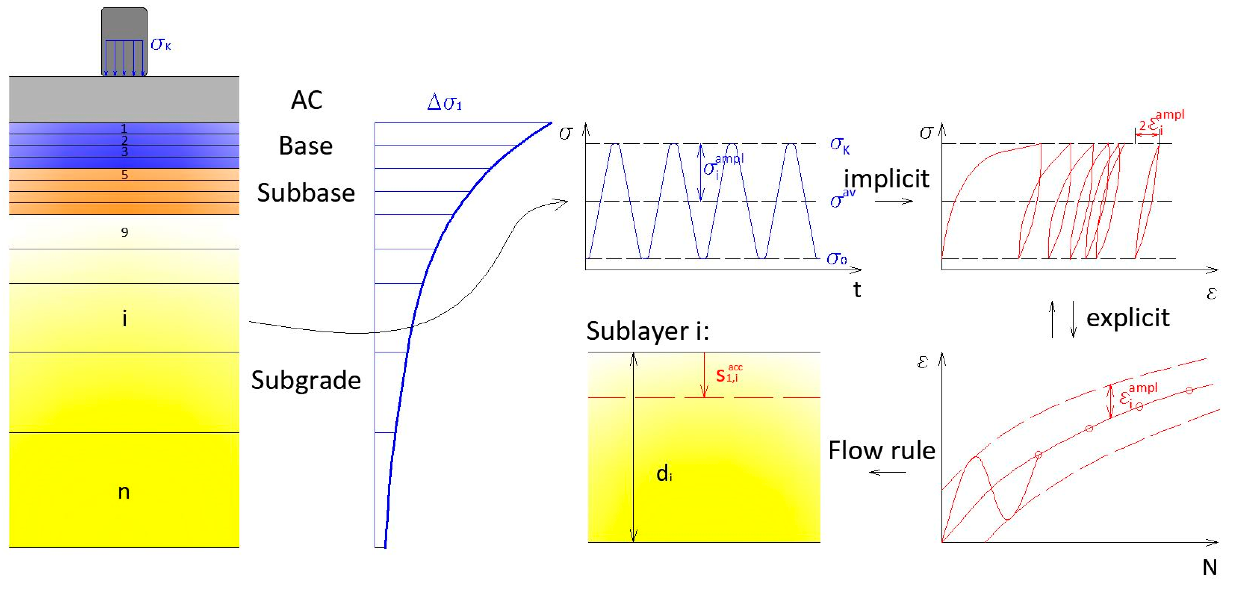
2.1. Explicit and Implicit Methods

The determination of permanent deformations has two fundamental approaches. Implicit methods directly calculate each cycle using a material model based on stress–strain increments ( σ ˙ ε ˙ ) and the residual deformation appears as a “by-product” of the calculation. The biggest disadvantage of these methods is that the calculation (integration) and material model errors are gradually accumulated with each load cycle; therefore, they can only be used reliably for N < 50 cycles [17].
Due to the above reasons, explicit calculation methods come to the fore in case of high-cycle loading. Instead of calculating the deformation trajectory at each load step and each cycle, the accumulated permanent deformation ( ε a c c ) is calculated in pseudo-time. The procedure is similar to creep and viscoplastic models, but instead of time (t), the number of cycles ( N ) is used. Explicit methods are empirical in nature, as the observed behaviour of the soil in the laboratory is described with mathematical formulae.

2.2. HCA Model

The basic principle of the HCA model is to combine the increment-based ( σ ˙ ε ˙ ) advanced implicit material model and the cycle number–permanent deformation ( N ε a c c ) explicit model. As a final result, the HCA model gives the accumulated strain ε a c c as a vector quantity under a cyclic loading with an N-number of constant stress amplitudes. The HCA model requires the void ratio, the mean effective normal stress, the stress state, and the cyclic strain amplitude ( ε a m p l ) as input parameters. The latter is implicitly calculated using a conventional material model by gradually increasing the cyclic stress and calculating the strain amplitude as the sum of the strain increments. Then, the strain amplitude is used as input to determine explicitly the permanent deformation under a cyclic load with an N-number of constant stress amplitudes. The model is presented in detail in the habilitation of [18]; hereinafter, only the most important calculation steps are discussed.
In the first step, the strain amplitude ε a m p l is determined due to q a m p l in a traditional implicit way, which is to be interpreted as the vector sum of the vertical and horizontal strains (1). The strain amplitude is defined as the mean value of the strains calculated at qmax–qmin points.
ε a m p l = ( ϵ 1 a m p l ) 2 + ( ϵ 2 a m p l ) 2 + ( ϵ 3 a m p l ) 2
Then, the calculation switches to the explicit part of the HCA model, in which the permanent strains due to the ΔN cycle package are determined with the above-defined ε a m p l . Since the soil structure and state parameters change in the long term, the explicit calculation is interrupted from time to time and the implicit analysis is repeated in control cycles in order to continue the explicit calculation for another ΔN cycle package with the actual value of ε a m p l .
In many constitutive models, when a stress path touches the yield surface, a plastic strain occurs. If the model takes hardening into account, then the yield surface shifts. For the HCA calculation, any suitable constitutive relationship such as plastic yield surface or strain hardening might be considered. The direction of the strain (e.g., volumetric or deviatoric) will be described with a flow rule. The difficulty of high cycle accumulations models is that the intensity of loading is somewhat moderate, and a cyclic plastic strain develops over the years of service due to the thousands and millions of load repetitions although the static yield requirements are not satisfied. For the general case, the strains are determined using the basic constitutive equation of the HCA model Equation (2)
σ ˙ = E   :   ( ε ˙ ε ˙ acc ε ˙ pl )
where
σ ˙ is the Cauchy stress tensor;
ε ˙ is the total strain rate;
ε ˙ a c c is the accumulated strain rate;
ε ˙ p l is the plastic strain rate, which starts to accumulate when the loading reaches the yield surface;
E is the stress-dependent elastic stiffness matrix.
Equation (2) gives the change in the stress (e.g., increase in pore pressure in undrained conditions, σ ˙ 0 ,     ε ˙ = 0 ) or strain (e.g., accumulated plastic strain in drained conditions, σ ˙ = 0 , ε ˙ 0 ) depending on the boundary conditions. In the analysis performed for this research, the latter boundary conditions are valid since drained conditions and sufficiently deep groundwater level were assumed. In this research, it is assumed that the stress path might only touch the yield surface during construction or by the first regular load cycle. Therefore, no static plastic strain develops during the repeated cyclic loading, so that ε ˙ p l = 0 . Thus, Equation (2) is simplified to ε ˙ a c c = ε ˙ . Refs. [10,18] provide further information on the plastic constitutive relationships of the HCA model.
The HCA model gives the rate of accumulation as a vector quantity, so in addition to the scalar magnitude of the strain, a flow rule is also needed to specify the direction of accumulation (m), i.e., to specify the deviatoric εq and volumetric εv parts of the strain. These can be used to determine the vertical strain components needed for the settlement analysis.
ε ˙ acc = ε ˙ a c c
The scalar part of the rate of accumulation can be determined using the other basic constitutive equation of the HCA model Equation (4), which is given as the product of five empirical factors. The f a m p l , f ˙ N , f p , f Y , and f e account for the influence of strain amplitude, the number of cycles, the mean normal stress, the mean stress ratio, and the void ratio, respectively. In some cases, a sixth term is also included in the equation, which describes the polarization of the cyclic loading f π . However, this factor can be neglected in most practical applications and can be taken as 1.0 based on the recommendation of [18].
ε ˙ a c c = f a m p l   f ˙ N   f e   f p   f Y   f π
The above-mentioned five f i functions can be described with seven C i material constants. Table 1 provides details of the constitutive relationships of the HCA model.
In addition, the critical friction angle φ c c is also needed to define the flow rule and f Y , which is not necessarily the same as the critical friction angle φ c that can be calculated from the monotonic CU triaxial test. In this research, the recommendations of [11] were used to determine the critical friction angle φ c c of the cyclic flow rule.

2.3. Direction of Accumulation

Based on laboratory test results, Refs. [11,19] found that the flow rule of MCC is approximately valid for sandy soils in the case of cyclic loading, so the vector of cyclic flow is mainly governed by the ratio of deviatoric and hydrostatic stresses η a v = q a v / p a v describing the average stress state. The relationship between the number of cycles and the strain rate ratio for a large number of cycles (105–2 · 106) was investigated by [11] on 22 different particle size distribution curves of clean quartz sand. Laboratory tests showed that the findings in [19] are somewhat inaccurate, as the plastic strain accumulation vector inclines towards the p axis, i.e., towards the volumetric strain, as the number of cycles increases. However, the MCC model is acceptable as an approximation for isotropic soils, since there are basically no shear strains in the case of η a v = 0, while only shear strains develop in the case of η a v = Mc. In this research, the MCC flow rule was applied to the sandy subgrade described in Section 4. Tests carried out on crushed stone base curse by [20] showed that, unlike sand, the material behaves anisotropically under compaction, so the flow rule of the MCC does not apply. Therefore, an anisotropic flow rule presented in [20] was used in this research for the base and subbase layers.

2.4. Determination and Calibration of the HCA Parameters

The calibration of Ci parameters is well-documented for the HCA model [13,21,22]. Based on these, there are three possible methods for determining these parameters. In the first case, at least 11 drained cyclic triaxial tests will be performed, which is quite time and work consuming. In the simplified procedure, Ce, Cp, CY, and Campl are determined with correlations and CNi parameters are calibrated using a single cyclic drained triaxial test. In the simplest approximation procedure, all parameters are determined using correlations based on particle size distribution tests (d50 and CU).
Because no additional laboratory tests were performed for this research, the latter simplified procedure is presented in detail below. The simplified calibration procedure discussed in the papers of [21,23] was developed on clean subangular quartz sand and gravel soils with no fines content. The samples had a coefficient of uniformity CU between 1.5 and 8.0 and a d50 between 0.1 mm and 3.5 mm, and the maximum cycle number was Nmax = 2 106. The maximum number of cycles of 2 million is an outstanding upper value compared to similar tests found in the literature. The running time of a single cyclic triaxial test in this case is approx. 23 days, during which technical problems may occur even despite the greatest precautions, e.g., water leaks from the triaxial cell into the sample via diffusion [23]. The 2 million cycles used in the laboratory can therefore be considered the upper limit of technical reliability. However, road pavements can be subjected to a higher number of load cycles. Since the behaviour of the soil is not known in the range greater than 2 10 6 cycles, the assumptions corresponding to the range of N > 2 10 6 should be treated cautiously and with appropriate criticism, as the validity of the Ci parameters is uncertain.
The boundary conditions of the particle size distribution discussed above are not valid for the crushed stone base and the subbase courses; therefore, the HCA parameters should be determined directly via laboratory testing of these layers [13]. The tests were performed on unbound crushed stone; and the particle size distribution curve of the material is in accordance with the Colombian Road Specifications. In the absence of literature data, it was assumed that the HCA parameters are also valid for the subbase course.

3. The Developed Layered Calculation Method

3.1. Basic Principles

The HCA model was originally implemented in the finite element program ABAQUS. Implicit calculations are generally time and work consuming, and implementation of the HCA model also requires a high level of programming skills and mechanical knowledge. A number of technical difficulties are documented in [24] when implementing the HCA model in the geotechnical finite element software Plaxis 2D V20. In order to make the application of the HCA model easier for practising engineers, simplified layered models were developed in MS Excel for shallow foundations under vertical cyclic loading and pile foundations under horizontal cyclic loading [25,26,27]. These layered models do not require finite element calculations, so the results can be quickly obtained without the need for any special software. The layered model is very useful for parametric studies or scheme design since the effect of different parameters on the settlement can be quickly investigated.
In this research, a simplified calculation model was developed in MS Excel on the analogy of the layered models, which can determine implicitly the strain amplitude ( ε a m p l ) in the layers (crushed stone base course, subbase course, and subgrade) beneath flexible pavements based on the theory of elasticity, the accumulated permanent strain ( ε a c c ) explicitly using the HCA model and the rutting depth under cyclic traffic loads.
The simplified calculation model works similarly to the layered models that are generally used for settlement calculations as the subsoil is divided into several sublayers. Then, stress distribution under the axle/wheel load is determined and the additional vertical load Δσ1,i in each sublayer is calculated. The strain amplitude in the centre line of each sublayer ε i a m p l (mean of the values at the top and the base of the sublayer) is determined via the mean normal stress, relative density, and strain-dependent nonlinear stiffness. Then, the accumulated permanent strain ε i a c c is calculated in each sublayer using the εiampl as input parameter, and compression of each sublayer is obtained by multiplying it with the thickness and the associated cyclic flow rule: s1,iacc = m1 * εiacc di. The direction of the accumulation was determined following the MCC flow rule in the subgrade, and using the anisotropic flow rule of [20] for the base and subbase courses. The total settlement or rutting depth is then obtained as the sum of the compression of each sublayer Σs1,iacc. The principles of the layered model are summarized in Figure 1.

3.2. Calculation Steps

The steps of the implicit calculation part can be summarized as follows. Subscript “i” refers to the number of the sublayer, and subscript “j” refers to the load step.
  • The vertical and horizontal stresses due to the own weight of the soil are determined;
  • σ 1 , i =   Σ γ i h i ;
  • σ 3 , i = σ 1 , i K x y , 0 , i , where K x y , 0 , i is the coefficient of earth pressure at rest by also considering overconsolidation;
  • The additional vertical load in each sublayer Δ σ 1 , i due to the wheel load is determined as the function of the geometry and stiffness of the sublayer;
  • The additional horizontal load is determined from the additional vertical load Δ σ 3 ,   i , j = Δ σ 1 ,   i , j K x y , i , j , where K x y , i , j is the coefficient of earth pressure considering overconsolidation and the incremental loading;
  • The additional vertical strain is calculated from the additional stresses, mean normal stress, relative density and strain-dependent stiffness: Δ ϵ 1 , i , j = Δ σ i , j E i , j ( p i , j ,   e ,   γ i , j a m p l ) . Because the incremental strain is the function of stiffness, and stiffness is the function of strain, iteration shall be used to determine the strain increment;
  • The total vertical strain and strain amplitude are calculated as the sum of increments in each sublayer: 2 ε 1 , i a m p l = Δ ϵ 1 , i = Σ ϵ 1 , i , j ;
  • The total horizontal strain and strain amplitude are calculated from the vertical strain and the ratio of horizontal strains ϑ in each sublayer: 2 ε 3 , i a m p l = Δ ε 1 , i ϑ = Σ ϵ 1 , i , j ϑ ;
  • Then, the elastic strain amplitude ε i a m p l is obtained using Equation (1);
  • For the base and subbase courses, the above implicit calculation method is simplified to the extent that the stiffness is taken into account with the MR resilient modulus, which is independent of the void ratio and strain level.
The explicit calculation part can be summarized as follows, where subscript “i” refers to the number of the sublayer, and subscript “k” refers to the packages of cycles.
11.
I mean normal stress and stress state ( p i a v ,   η i a v ) is determined in the center line of sublayer “i” and then the factors independent of the number of cycles f p ,   f Y and f ˙ N B are calculated;
12.
In the next step, factors of Equation (4) that depend on the number of cycles are obtained: f a m p l   from the actual ε i a m p l , f ˙ N , k A from the actual g k A and f e   from the actual e void ratio;
13.
The accumulated strain rate ε ˙ i acc is calculated using Equation (4). In the case of drained conditions, Equation (2) becomes ε ˙ i a c c = ε ˙ i ;
14.
The strain increment due to Δ N cycles is determined by Δ ε i = ε ˙ i Δ N , then ε i ( N +   Δ N ) = ε i ( N ) + Δ ε i ;
15.
Calculating the rate of the preloading variable g ˙ A with the actual value of g k A  ;
16.
The actual value of g k A is updated due to Δ N load cycles by Δ g i A = g ˙ i A Δ N ,   then   g i A ( N + Δ N ) = g i A ( N ) +   Δ g i A ;
17.
Vertical strains are calculated using the flow rule ε 1 , i , k a c c = ε i , k a c c m 1 , then compression of each sublayer by s 1 , k a c c = Σ ε 1 , i , k   a c c h i ;
18.
Volumetric strain increment is determined due to Δ N cycles, then the new void ratio is obtained by ε v , i , k a c c = ε i , k a c c ( m 1 + 2 m 3 ) , e i ,   N + Δ N = e i , N ε v , i , k a c c ( 1 + e i , N ) ;
19.
The e i ,   N + Δ N characterizing a denser state results in a higher stiffness E i ,   N + Δ N ( p , e ,   γ i , j a m p l ,   ϑ i ) , thus points 6.–9. of the implicit calculation are repeated;
20.
Steps 12.–18. of the explicit calculation are repeated until the goal value of a number of cycles.

4. Analysed Pavement Structures and Material Models

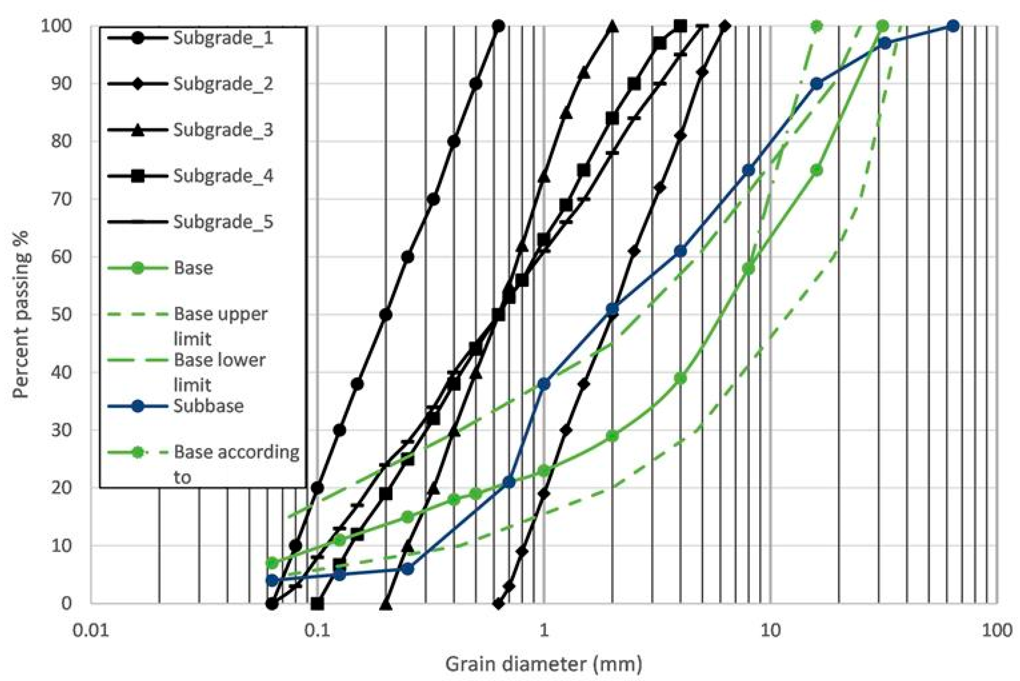
4.1. Analysed Pavement Structures

The goal of this research was to determine the accumulated permanent strains and rutting depths in the standardized pavement cross-section according to [1] shown in Table 2 due to repeated passes of a standard axle. The cross-sections are composed of four layers (sand and gravelly sand subgrade course, granular subbase course, crushed stone base course, and asphalt course). The subgrade comprises quartz sand and gravelly sand of subangular particles; the particle size distribution is shown in Figure 2, and it was assumed to have a relative compaction of R.C. = 93%. The subgrade is overlain by a subbase course of 20 cm thickness. The material of the subbase is discussed in detail in the thesis of [28], and its particle size distribution is presented in Figure 2. The subbase is overlain by an unbound well-graded crushed stone base course of 20 cm thickness (Table 2); this material is described in detail in the works of [20,29]. Particle size distribution of the pavement layers is shown in Figure 2, whereas their properties are summarized in Table 3. The base course is overlain by an asphalt course of traffic load class-dependent thickness.

4.2. Materials and Their Properties

The asphalt course was considered a homogeneous layer, which can be characterized by its traffic load class-dependent thickness, Young’s modulus, and Poisson’s ratio. The stiffness of the asphalt was taken to be constant ( E a = 4.000 MPa, υ a = 0.35) according to the equivalent temperature [30]. Poisson’s ratio of the subbase and base courses was taken from [30]. The Poisson’s ratio in the subgrade is not constant either in the sublayers or during loading, and its value can be calculated based on the relationships of the theory of elasticity from the shear and constrained (oedometer) modulus.
It is assumed that the subbase course has a relative compaction of R.C. = 95%. The bearing capacity (E2) modulus of the subbase material based on finite element calculation [31] is approx. An amount of 150 MPa, thus an E2,sb of 60 MPa, can be expected on top of the subbase. It is assumed that the crushed stone base course has a relative compaction of R.C. = 96%. The bearing capacity (E2) modulus of the crushed stone material based on finite element calculation [31] is approx. An amount of 230 MPa, thus an E2,b of 125 MPa, can be expected on top of the base course, which complies with the international practice of flexible pavement construction. Because there was no Proctor test available for the subgrade, it was assumed that ρdmax corresponds to a void ratio of e = 0.95 emin. The particle size distribution of the analysed layers is shown in Figure 2, whereas their properties are summarized in Table 3.
The HCA parameters of the subgrade were calculated using the relationships of [18,32,33] from d50 and CU. The input parameters for the subbase and base courses were determined considering the tests of [20]; the only exception is the Ce parameter as it was calculated from the actual emin of the subbase using the difference of emin-The HCA parameters of the subgrade were calculated using the relationships of [18,33,34] from d50 and CU. The input parameters for the subbase and base courses were determined considering the tests of [21]; the only exception is the Ce parameter as it was calculated from the actual emin of the subbase using the difference of emin − Ce in the crushed stone base. The HCA parameters used in the analysis are summarized in Table 4. The notations in brackets for the subgrades correspond to the same notation as the examined soils in [18].

4.3. Material Model of the Implicit Calculation

The HCA model is sensitive to the input of ε a m p l , so it is important to calculate it as accurately and carefully as possible. Generally, the hypoplastic material model with small strain stiffness is used for the implicit calculation part [10]; however, in [27] an isotropic elastic material model according to [34] is used in addition. In [27] it is noted that ε a m p l can be determined by basically any material model. However, the (elastic) deformations should be modelled as precisely as possible; therefore, the material model used should take into account the nonlinearity of stiffness depending on relative density, mean normal stress, and small strains.
In the implicit calculations of this research, the subgrade was modelled as a nonlinearly elastic material with a stiffness depending on the void ratio, the mean normal stress, and the strain level. Small strain shear modulus Gmax and constrained (oedometer) modulus of the subgrade were calculated using the relationships of [18,32,33] from d50 and CU. The degradation curve was determined according to the relationships presented by [32]. As stiffness ( G , E , M , υ ) depends on the mean normal stress and strain, it changes constantly and should be determined for each sublayer in each package of cycles in every load increment. Moreover, the actual strain increment and the corresponding actual stiffness should be determined by iteration for each load step.
For unbound granular base and subbase materials, the resilient modulus MR can be calculated using the following nonlinear elastic relationship [35]
M R = k 1 θ k 2
where
M R is the resilient modulus;
θ is the bulk stress;
k 1     and k 2 are material constants.
Table 5 shows the typical range of k 1 and k 2 parameters. In the absence of laboratory tests, the k values should be determined by engineering judgment based on the drainage conditions and material characteristics.
The stiffness of the crushed stone base and subbase were determined using Equation (5). The “k” parameters for the crushed stone base were taken as the mean of the ranges given in Table 5 ( k 1 = 5500 psi, k 2 = 0.6), whereas they were taken slightly above the mean for the subbase course ( k 1 = 5000 psi, k 2 = 0.55). For the subbase, the slightly higher values are justified by the fact that the particle size distribution and type of the material (50% crushed stone) make the subbase of higher quality than conventional subbase materials. It is also noted that the resilient moduli calculated by the above assumptions (MR,sub~150 MPa, MR,base~210 MPa) show good agreement with the back-analysis of plate load tests presented in [31]

5. Implicit Calculation Model and Comparative Study

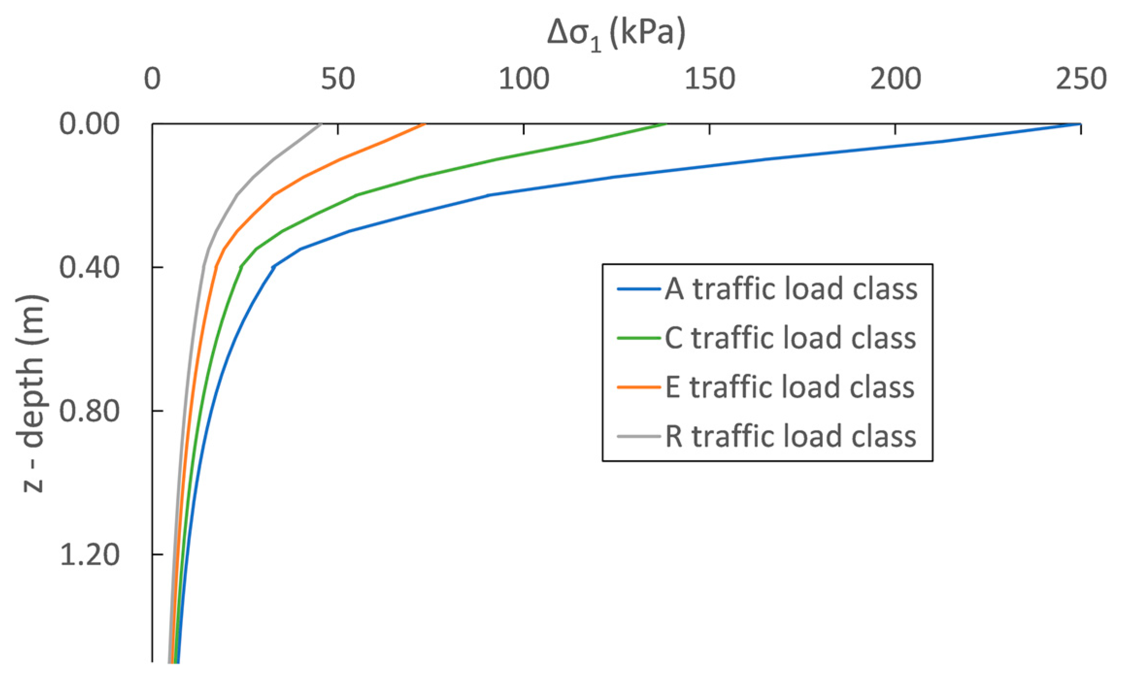
5.1. Vertical Stress Distribution

Traffic load is characterized by the standard axle load, which is taken as 10 tons. The axle load is distributed evenly on the two circular wheels, each with a diameter of 30 cm, so the additional vertical stress will be Δ σ 1 = 707   kPa on top of the asphalt course. This stress is distributed proportionally to the thickness of the layers and their relative stiffnesses (E, v). The stress distribution and the additional stress Δ σ 1 , i in each sublayer are determined based on the theory of multi-layered elastic isotropic infinite half-space derived by Boussineq. Since the model includes the small strain behaviour of the subgrade, the layer’s stiffness significantly depends on the vertical stress increment. However, it is also true that the stress distribution in the layered elastic half-space is determined by the stiffness of the individual layers as an input parameter. The stiffer layers attract proportionally higher additional stress, as a result of which the stiffness of them starts to decrease due to the increasing strain level. Consequently, the final stress distribution should be determined by iteration.
Figure 3 shows the distribution of the additional vertical stress with depth for traffic load classes A-C-E-R. For traffic load classes B-D-K, the distribution curves fall between the adjacent load classes, so they are not displayed in the figure for better visibility. As the figure also shows, the thickness of the asphalt course has a significant influence on the stress distribution. In traffic load class A, the crushed stone base, the subbase, and the subgrade are subjected to approx. 5 times, 4 times and 2.5 times higher additional vertical load, respectively, than in traffic load class R. The curves converge well, and, although Figure 3 is somewhat deceptive, even at the depth of 1.5 m the difference is still around 50% between traffic load class A and R.

5.2. Horizontal Strain Ratio

The vertical strain of the ith sublayer due to additional vertical stress Δσ1,i can be calculated from the three-dimensional Hooke’s law Equation (6).
Δ σ 1 , i = E i ( 1 + υ ) ( 1 2 υ )   [ ( 1 υ ) · ε 1 , i + υ · ε 2 , i + υ · ε 3 , i ]
where:
E is the Young’s modulus,
υ is the Poisson’s ration.
Let us determine the lateral strains, ε 2 and ε 3 , in the function of vertical strain by assuming that the strains in the two lateral directions are the same due to the axisymmetric conditions Equation (7). Combining Equations (6) and (7) and rearranging it to ε , gives Equation (8).
ε 2 = ε 3   = ϑ ε 1
where ϑ is the ratio of lateral and vertical strain.
Δ ε 1 , i = Δ σ 1 , i E i ( 1 + υ ) ( 1 2 υ ) 1 υ + 2 υ ϑ
The dependence of the ϑ factor on depth is discussed by [36] for shallow foundations under static load. This relationship did not provide satisfactory agreement with the comparative analysis, so a new relationship was developed for ϑ ( z ) in [31] for each pavement layer. Ref. [31] presents a finite element analysis for traffic load classes A-R where the load was gradually increased in steps of 2 tons, and the ϑ ( z ) relationship was obtained by curve fitting on the results using the least squares method. In this research, the ratio of horizontal strains is described by the ϑ ( z ) relationship presented there.

5.3. Coefficient of Earth Pressure

An increase in the horizontal earth pressure reduces the permanent strains. The higher horizontal stress increases the mean normal stress and thus the stiffness of the soil E = f ( p ), so the value of f a m p l also decreases due to the decreasing cyclic strain amplitude ε a m p l . Although its effect is smaller, the increasing mean normal stress also reduces the degree of accumulation via the f p function. Accordingly, the horizontal stresses should be taken into account as precisely as possible. The soils beneath road pavements are considered to be overconsolidated, thus conventional coefficients of earth pressure are not valid for them. The overconsolidation is caused by the traffic and compaction loads during construction. The stresses generated by these actions are many times higher than the stresses occurring during the operation of the road. Consequently, OCR >> 1 and thus Kxy  K0NC. Ref. [31] performed finite element analysis for the determination of the Kxy(z) relationship for traffic load classes A-R by increasing the load in 2-ton steps; the relationship for the crushed stone base, subbase and subgrade was obtained by curve fitting on the results using the least squares method. The horizontal coefficient of earth pressure in this research is calculated using the functions and parameters presented in that paper.

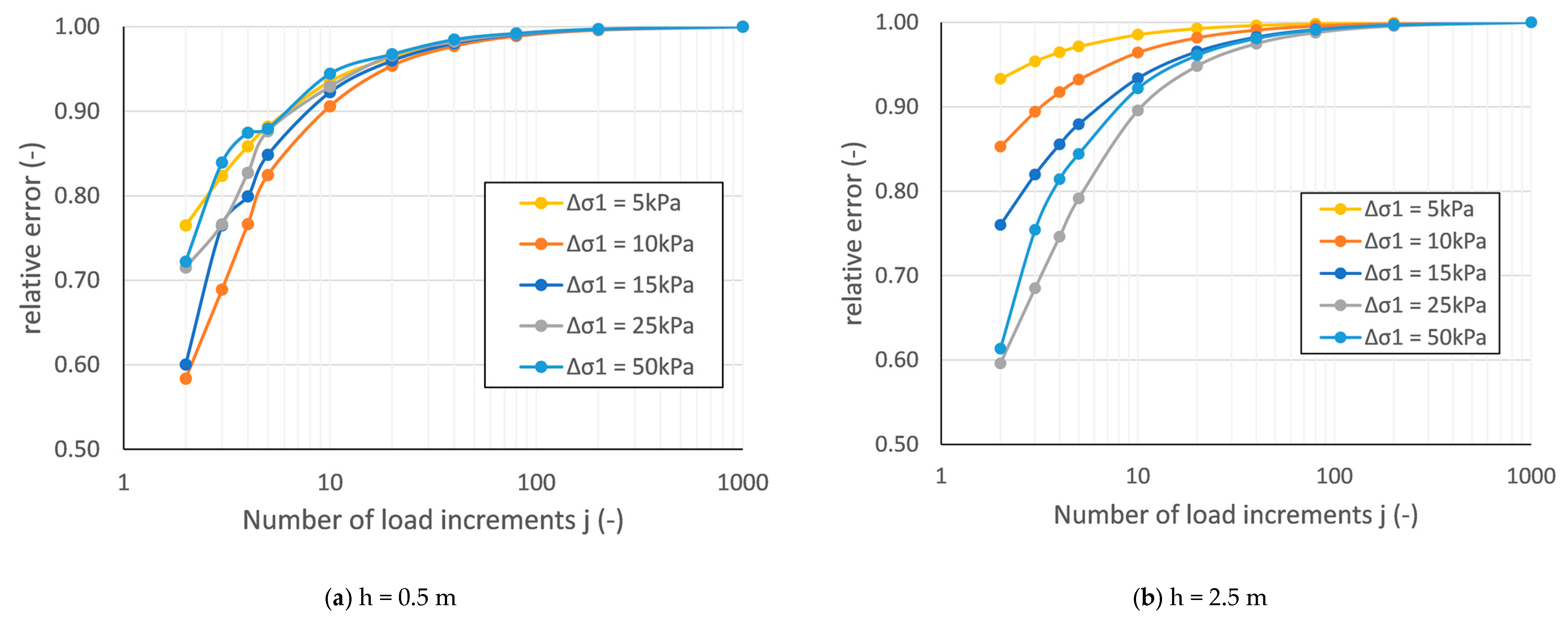
5.4. Number of Load Increments

Since the applied material model is nonlinearly elastic, the result depends on the number of load steps. In the model, the load was divided into j equal parts and then it was applied in uniform steps of Δ σ 1 / j . A parametric study was performed on soils with different thicknesses and loading and the number of load steps was changed between j = 2-3-4-5-10-20-40-80-200-1000, and then the strain Δ ε 1 was determined due to Δ σ 1 load. The relative error, i.e., the ratio of the strain calculated with the actual “j” and belonging to j = 1000 converges to 1.0 over time, so the calculated strains are almost the same, and from an engineering point of view, there is basically no difference between the results. The relative error was calculated in three different depths for five load increments and 10 load steps. The relative error obtained for depths of h = 0.5 m and h = 2.5 m is presented in Figure 4 as the function of the number of load steps. The relative error quickly converges to 1.0; the difference is already negligible at j = 40. The value of relative error ranged from 0.97 to 1.00 in the entire analysed spectrum for j = 40. Due to the above reasons, the loading step of j = 40 was used in all the calculations, which already yields sufficiently accurate results from an engineering point of view.

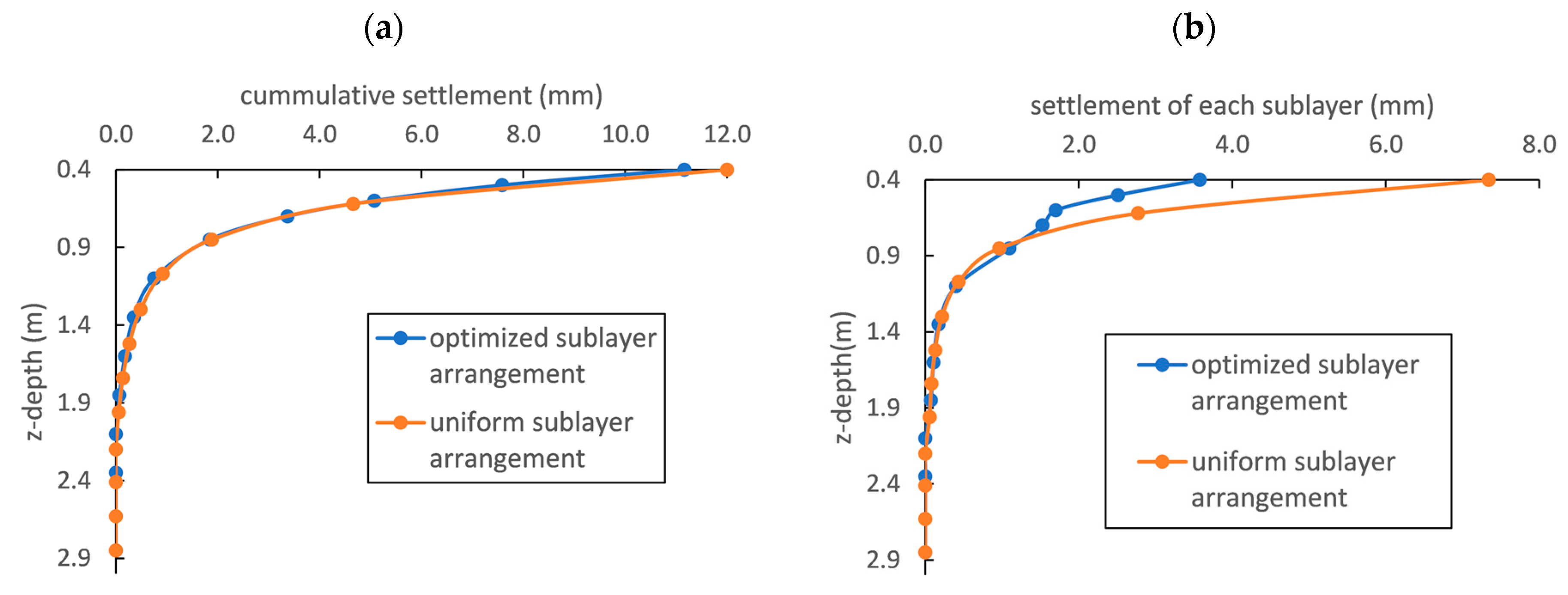
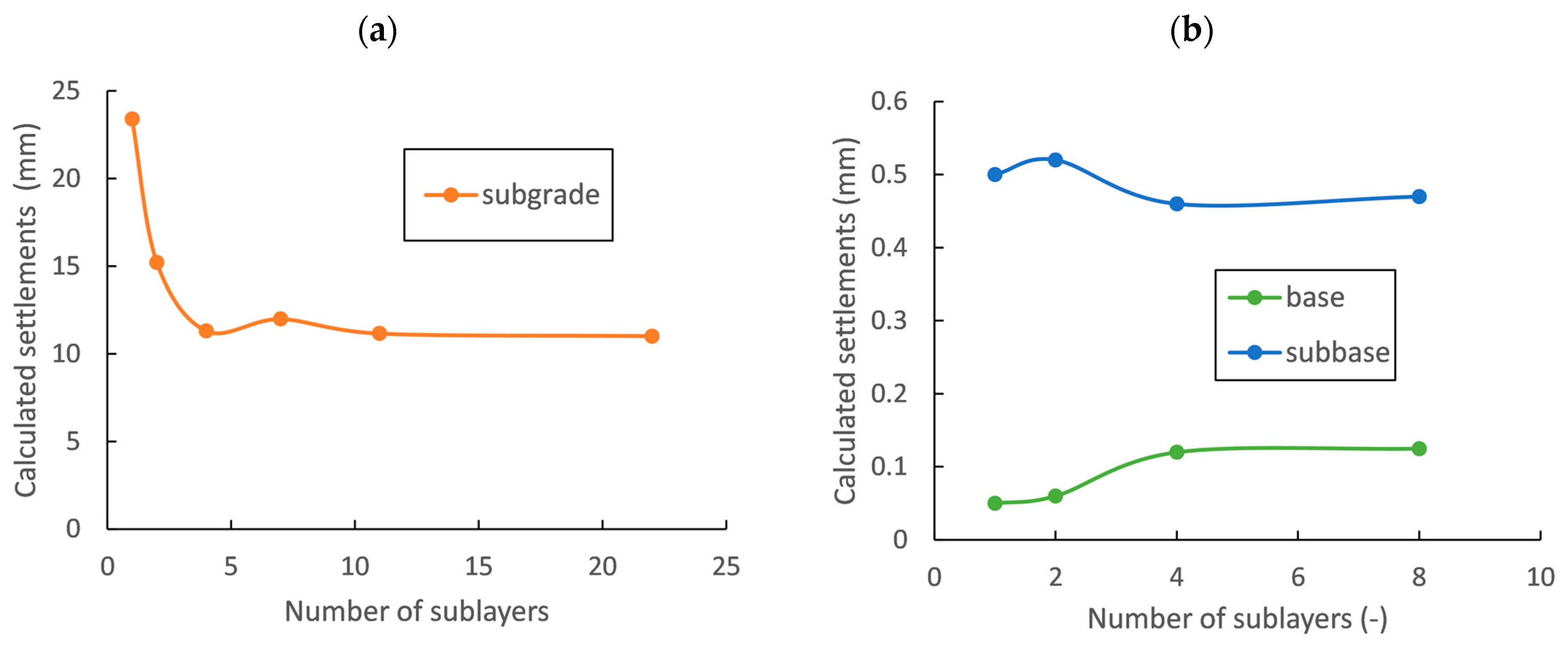
5.5. Number and Arrangement of Layers

After clarifying the implicit part of the calculation, an answer had to be given to the question of how to discretize the soil, i.e., how the number and distribution of sublayers affect the settlement. The goal was to determine the minimum number of sublayers, with which the settlement no longer changes significantly. A parametric study was performed for traffic load class C and compression was evaluated in each layer with an increasing number of sublayers.
In the first step, the discretization of the subgrade was analysed. The sublayers can be distributed evenly with depth, i.e., all sublayers have the same thickness. Since the input parameters and thus the strain amplitude changes rapidly at the top of the layer, this leads to an overestimation of the settlement. Discretization of the layers was therefore optimized in such a way that, although the number of sublayers remained the same, the sublayers were thinner at the top of the layer, whereas they were thicker at the bottom; from top to bottom: 0.1 m–0.1 m–0.1 m–0.15 m–0.25 m–0.25 m–0.25 m–0.25 m–0.25 m–0.25 m–0.5 m. Figure 5 shows the cumulative settlements with depth and the compression of each sublayer for both types of discretization. The cumulative settlement is almost 8% higher in the case of uniform discretization, and this develops in the top approx. 0.5 m zone of the layer. The figures also show that the cumulative settlement is smaller in the deeper layers in the case of uniform discretization. The reason behind this is that the value of ε a m p l is very close to 10−5, below which cumulative strains do not develop. Since uniform discretization describes the deeper layers with greater accuracy, settlement starts to accumulate from the depth of approx. 1.95 m, compared to the 2.1 m depth of the optimized model. Nevertheless, the optimized model describes the settlement more accurately in the most important depths.
In the next step, the discretization was optimized to determine the necessary and sufficient number of sublayers. The developing settlements are shown in Figure 6 as the function of the number of sublayers (1-2-4-7-11-22). Since the sublayers were made thinner in the relevant places, an accurate result could already be obtained with a relatively small number of sublayers (from i = 4) and the correlation converges quickly. Based on the results, the subgrade was divided into i = 11 sublayers in the subsequent calculations, as above this further increase in accuracy was not experienced. The additional vertical stress, ϑ and K x y coefficient of earth pressure changes rapidly with depth in the crushed stone base and subbase courses, so a finer discretization is required than for the subgrade. The developing settlements are shown in Figure 6 as the function of the number of sublayers (1-2-4-8). It can be seen that there is no significant change starting from i = 4, so the subbase and base courses were divided into four sublayers in the model. Since the sublayer thickness of 5 cm is quite small and the input parameters change continuously with depth, a uniform discretization was applied in these courses.

6. Discussion of Layered Model Results

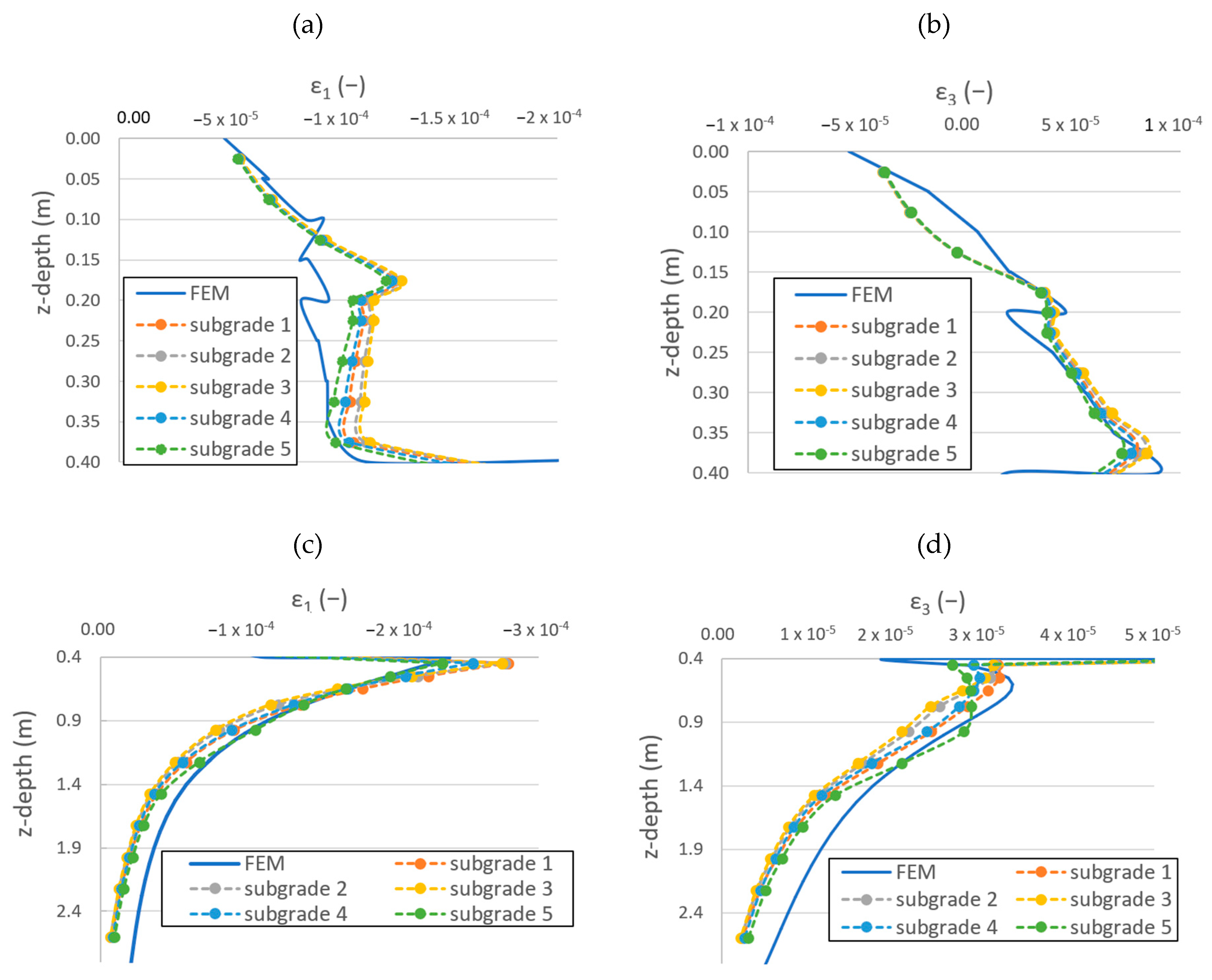
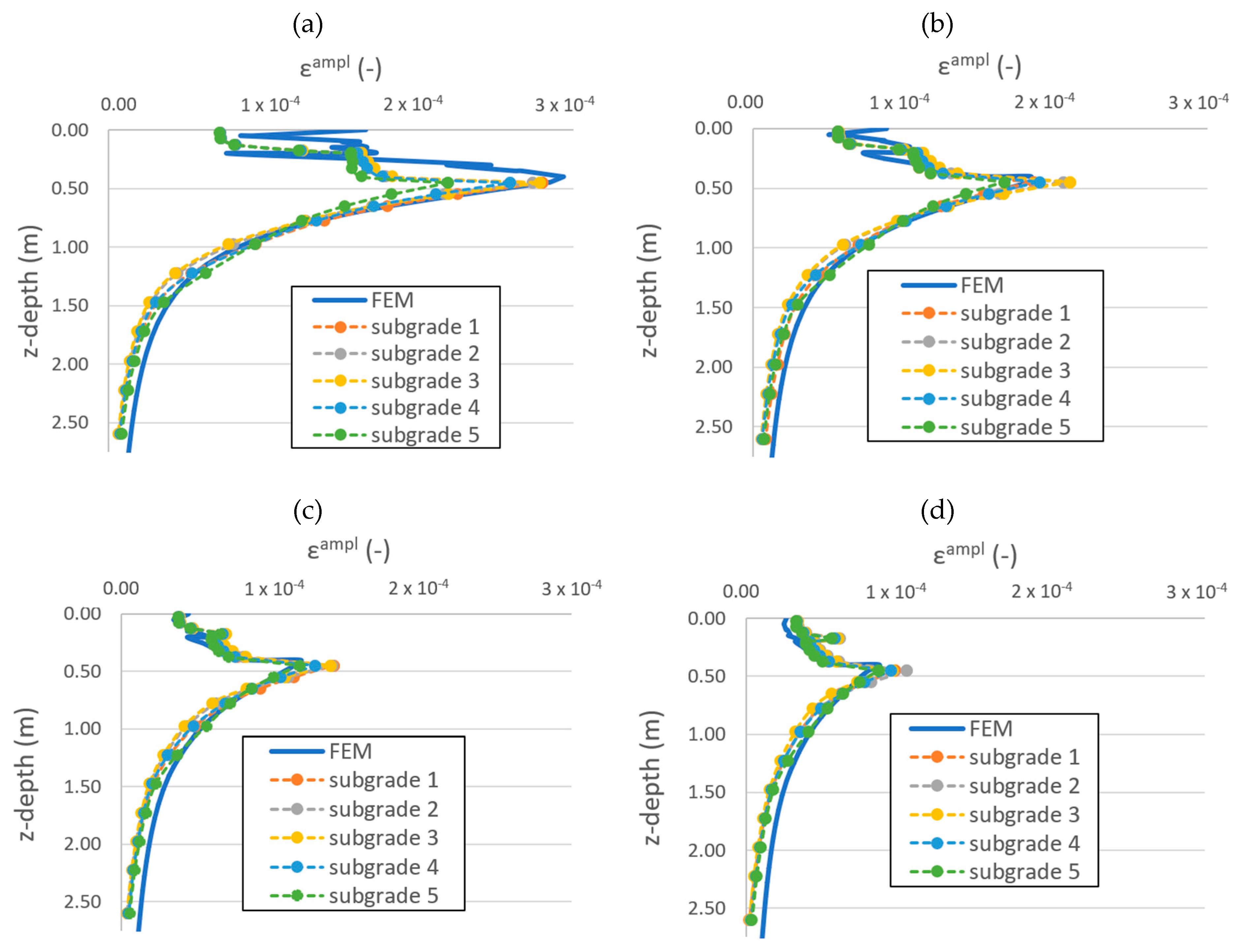
6.1. Implicit Calculation Results

Using the simplified layered method presented in Section 3, Section 4 and Section 5, ε1 and ε3 strains were determined for the traffic load classes A-R and the above-presented pavement layers under a standard axle load, and the results were compared with the finite element analysis results presented in [31]. Figure 7a,b show the vertical and horizontal strains in the base and subbase courses for traffic load class E. The ε1 values adequately approximate the vertical strain obtained by the finite element analysis, except for the boundary of the subbase and base courses. The shape of the functions is also satisfactory However, the simplified model predicts that the vertical strain decreases with depth in the subbase layer, whereas the finite element analysis shows that it increases slightly with depth Figure 7a. The minor horizontal strain almost perfectly matches the results of the finite element analysis (Figure 7b). Figure 7c,d show the results for the subgrade, where a good match between the results can be observed. The vertical strain is slightly overestimated in the top of the layer, whereas it is slightly underestimated in the lower portions. The horizontal strain is always underestimated except for the topmost part of the subgrade.
Although each strain component is of interest, focus is given to ε a m p l as the most important input parameter of the HCA model. Figure 8 shows the calculated ε a m p l for traffic load classes A-C-E-R and compares it with the results of the comparative finite element analysis. As expected, the greater the thickness of the asphalt course, which increases with traffic load class, the better the wheel load is distributed, thus the additional vertical stress acting on the underlying layers becomes significantly less. Accordingly, the strain amplitudes also decrease gradually in the higher traffic load classes (stronger pavements), and an almost three-fold difference is observed in the strain amplitude between classes A and R. The relationship between ε a m p l and depth and the shape of the functions are the same regardless of the traffic load class. As the figure shows, the results obtained by the simplified model agree well with the results of the finite element analysis.

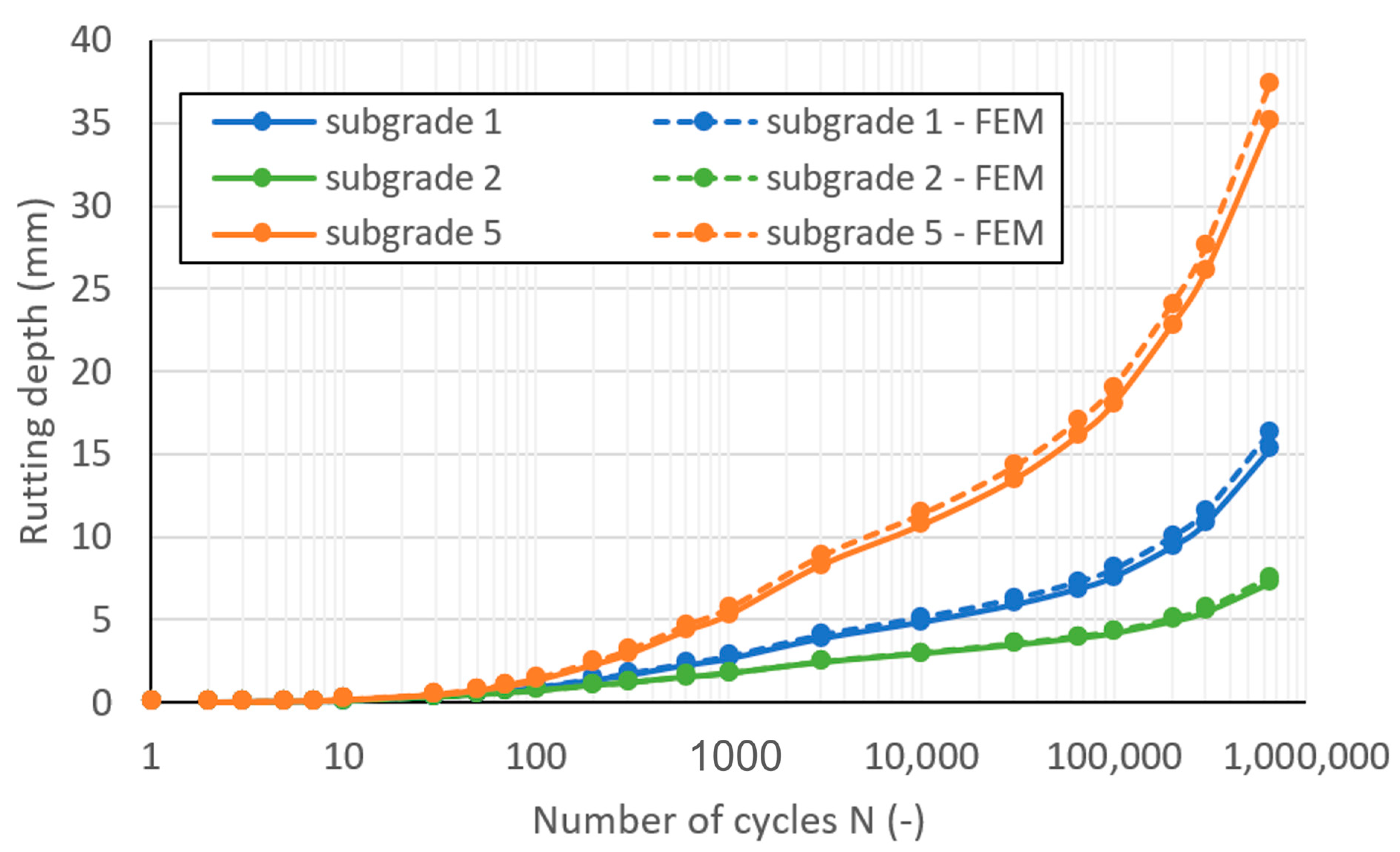
6.2. Comparison of Permanent Deformation Results between Layered and FE Model

Then, the rutting depth predicted by the HCA model in traffic load class C was analysed in the cases when the input parameters, such as pav, ηav, and ε a m p l are determined using the simplified layered procedure and when they are obtained from the finite element model. Since the selected finite element material model (HS-Small) does not take into account the increase in stiffness with increasing relative density, and thus would overestimate ε a m p l and εacc for a high number of cycles, the ε a m p l was reduced in the first cycle according to Equation (9). It was assumed that the strains are still proportional to the component of the Gmax relationship that contains the void ratio, and the strains at the beginning of the ith packages of cycles were calculated from the ratio of the void ratio at the beginning of the ith packages of cycles and the void ratio at the first cycle.
ε i a m p l = ε P l a x i s a m p l / ( a G e N = i . ) 2 1 + e N = i . ( a G e N = 1 . ) 2 1 + e N = 1 .
Figure 9 illustrates the obtained rutting depths with the number of cycles for traffic load class C. The results given by the simplified procedure and the finite element model are basically the same regardless of the soil type of the subgrade as the difference between the rutting depths of the two approaches at the end of the design working life is approx. 3–7%. The difference was of a similar magnitude for the other traffic load classes as well. Accordingly, it can be concluded that the simplified layered procedure presented above describes well the short-term behaviour of the subgrade under wheel load; therefore, it is suitable to provide an appropriate input for the HCA model.

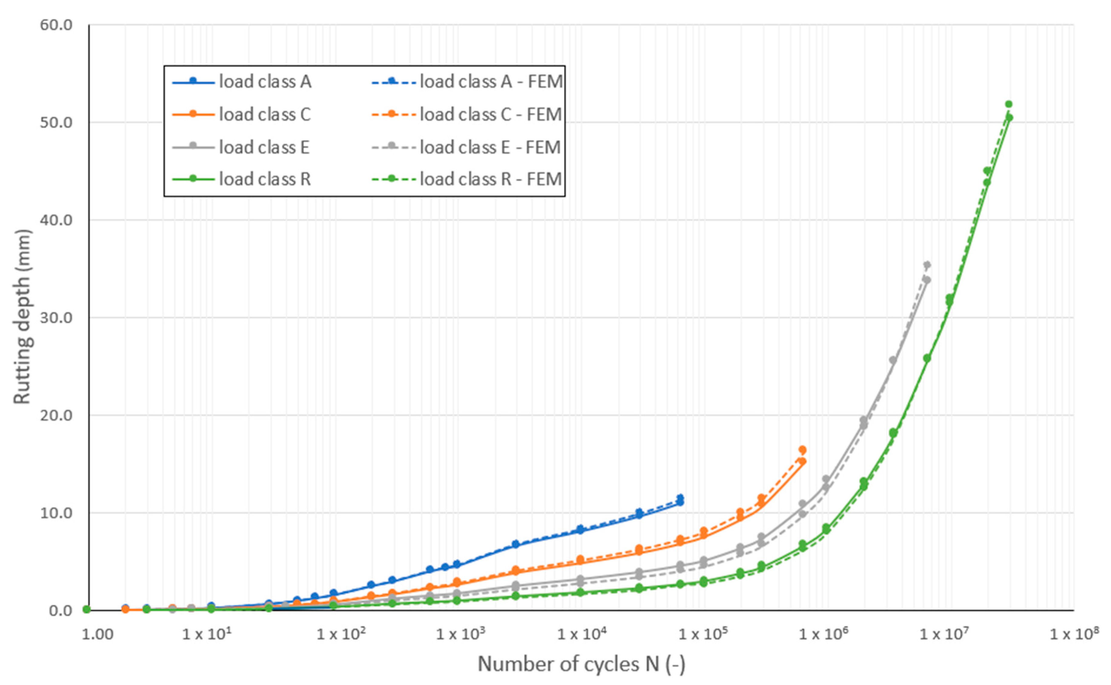
6.3. Effect of Traffic Load Class on Permanent Deformations

This section presents the residual rutting depth for subgrade 1 for each traffic load class as a function of the number of cycles, and a comparison is made between the results obtained by using the simplified layered model to determine the input parameters and by using the finite element model (Figure 10). As the figure shows, the rutting depth calculated from the input data of the simplified layered model approximates well the result of the finite element model regardless of the traffic load class. At the end of the design working life, the difference between the calculated settlements is approx. 2–5%.
The pavement structure of the traffic load classes was devised in such a way that the stresses resulting from the repeated passing of axles with different numbers of cycles cause the same fatigue in the asphalt course over the entire design working life. Based on Figure 10, this is not true for the rutting depths as at the end of the design working life, they increase with the traffic load class. However, the rutting depths are smaller in the higher load classes for the same number of cycles. This is logical since the thicker asphalt course of the higher traffic load class distributes the wheel load better, so smaller stresses reach the underlying layers, and therefore εampl will also be smaller. Consequently, the accumulated strains are smaller in the higher load classes for the same number of cycles. This means that in load class A at the end of the design working life, i.e., after 65,000 axle passes, the rutting depth is approx. four times the rutting depth of the class R at the same number of cycles. However, traffic load class R suffers approx. 4.6 times greater rutting depth by the end of the design working life as it is subjected to approx. 460 times more axle passes.

7. Conclusions

A calculation algorithm was developed in MS Excel, which implicitly calculates throughout the lifetime of the pavement continuously changing elastic strains ( ε a m p l ) developing in the different layers of a flexible pavement system, and by using the HCA model, explicitly determines the accumulated strains (εacc) and rutting depths sacc under repeated axle load in the axis of the wheel. The advantage of the presented method is that the rutting depth can be predicted solely based on literature data and basic particle size distribution parameters (d50, Cu, k1, k2, emin, and emax); therefore, it is suitable for parametric studies and quick preliminary designs, where the time- and cost-intensive laboratory tests and FE calculations are not available. For the sake of reliability, it is, however, necessary that for further pavement design, the HCA material parameters and the resilient behaviour of the soil layers are determined with time-consuming cyclic triaxial laboratory tests to obtain more accurate material input parameters.
The model considers the change in the horizontal earth pressure resulting from the preloading of the pavement during construction and the typical horizontal strain conditions of road pavements. The actual behaviour of the subgrade is taken into account by the stiffness depending on the relative density, the mean normal stress and strain level, while the behaviour of the crushed stone base course and subbase course is taken into account by a nonlinearly elastic k-Θ model depending on the normal stress.
Due to the nonlinear behaviour, the strains shall be determined in the incremental form ( σ ˙ ε ˙ ) . It was shown that the necessary and sufficient number of load steps is i = 40. The discretization of the layers, i.e., the required number and distribution of the sublayers, was also analysed. A parametric study was performed in the subgrade, which showed that more accurate results would be obtained if the sublayers were thinner at the top and thicker at the bottom instead of a uniform thickness (Figure 5). By changing the number of sublayers, a recommendation was made for the necessary and sufficient number of sublayers in the base, subbase, and subgrade courses, which are 4, 4, and 11, respectively. Finer discretization does not lead to a significant increase in accuracy.
The elastic strains calculated by the developed simplified layered model for five different subgrades and seven pavement structures were compared with the results of a reference finite element model [31]. It was shown that the developed simplified layered model can provide sufficiently accurate results for the strain amplitude εampl based solely on literature data and basic particle size distribution parameters (d50, Cu, k1, k2) without the need forfor finite element calculations (Figure 8). Depending on if the input parameters (εampl, pav, ηav) of the explicit model from the developed simplified procedure or the finite element calculations originate, the differences in the accumulated rutting depths for the traffic load class C with three different subgrades are approx. 3–7% (Figure 9). Similarly, the calculated rutting depths with the explicit model also show a good agreement (2–5%) regardless of whether the input parameters originate from the developed layered model or the reference finite element model (Figure 10).
Rutting depth in each traffic load class and subgrade type was calculated and plotted on a diagram as a function of the number of cycles (Figure 10). It was shown that the rutting depth at the end of the design working life increases with increasing traffic load class. However, for the same number of cycles, the rutting depths are smaller in the higher load classes.
It was shown that the permanent rutting depths due to traffic loads can be determined with sufficient accuracy using the developed simplified layered model for flexible pavements with different sections and subgrades. The future goal of this research is to perform additional parametric studies with the model and to explore which factors have the greatest influence on permanent settlement.

Author Contributions

Conceptualization, M.J.V. and J.S.; methodology, M.J.V. and J.S.; software, M.J.V. and J.S.; validation, M.J.V. and J.S.; formal analysis, M.J.V. and J.S.; investigation, M.J.V. and J.S.; resources, M.J.V. and J.S.; data curation, M.J.V. and J.S.; writing—original draft preparation, M.J.V. and J.S.; writing—review and editing, M.J.V. and J.S.; visualization, M.J.V. and J.S.; supervision, M.J.V. and J.S.; project administration, M.J.V. and J.S.; funding acquisition, M.J.V. and J.S. All authors have read and agreed to the published version of the manuscript.

Funding

This research received no external funding.

Data Availability Statement

The data that support the findings of this study are available from the corresponding author upon reasonable request.

Conflicts of Interest

The authors declare no conflict of interest.

References

  1. e-UT06.03.13 (ÚT 2-1.202); Aszfaltburkolatú Útpályaszerkezetek Méretezése És Megerősítése (Design of Road Pavement Structures and Overlay Design with Asphalt Surfacing). Útügyi Műszaki Előírás (Road Design and Specification Standard): Budapest, Hungary, 2017.
  2. FGSV Verlag. RStO Richtlinie für die Standardisierung des Oberbaues von Verkehrsflächen; FGSV Verlag: Köln, Germany, 2001. [Google Scholar]
  3. Powell, W.D.; Potter, J.F.; Mayhew, H.C.; Nunn, M.E. The structural design of bituminous roads. In Trrl Laboratory Report; Transport and Road Research Laboratory: Wokingham, UK, 1984. [Google Scholar]
  4. Shell. SPDM-PC User Manual. Shell Pavement Design Method for Use in a Personal Computer (Version 1994, Release 2.0); Shell International Petroleum: London, UK, 1994. [Google Scholar]
  5. Little, P.H. The Design of Unsurfaced Roads Using Geosynthetics. Ph.D. Dissertation, The University of Nottingham, Nottingham, UK, 1993. [Google Scholar]
  6. Gidel, G.; Hornych, P.; Chauvin, J.; Breysse, D.; Denis, A. A New Approach for Investigating the Permanent Deformation Behaviour of Unbound Granular Material Using the Repeated Loading Triaxial Apparatus. Bull. Lab. Ponts Chaussees 2001, 1, 5–21. [Google Scholar]
  7. Uzan, J. Permanent Deformation in Flexible Pavements. J. Transp. Eng. 2004, 130, 6–13. [Google Scholar] [CrossRef]
  8. Werkmeister, S. Permanent Deformation Behaviour of Unbound Granular Materials in Pavement Constructions. Ph.D. Értekezés, TU Dresden, Drezda, Germany, 2003. [Google Scholar]
  9. Niemunis, A.; Wichtmann, T.; Triantafyllidis, T. A High-Cycle Accumulation Model for Sand. Comput. Geotech. 2005, 32, 245–263. [Google Scholar] [CrossRef]
  10. Wichtmann, T. Explicit Accumulation Model for Non-Cohesive Soils under Cyclic Loading; Schriftenreihe des Institutes für Bodenmechanik der Ruhr-Universität Bochum: Bochum, Germany, 2005. [Google Scholar]
  11. Wichtmann, T.; Niemunis, A.; Triantafyllidis, T. Flow Rule in a High-Cycle Accumulation Model Backed by Cyclic Test Data of 22 Sands. Acta Geotech. 2014, 9, 695–709. [Google Scholar] [CrossRef]
  12. Wichtmann, T.; Niemunis, A.; Triantafyllidis, T. On the Determination of a Set of Material Constants for a High-cycle Accumulation Model for Non-Cohesive Soils. Int. J. Numer. Anal. Methods Geomech. 2010, 34, 409–440. [Google Scholar] [CrossRef]
  13. Wichtmann, T.; Niemunis, A.; Triantafyllidis, T. Simplified Calibration Procedure for a High-Cycle Accumulation Model Based on Cyclic Triaxial Tests on 22 Sands. In Frontiers in Offshore Geotechnics II; CRC Press: Boca Raton, FL, USA, 2010. [Google Scholar] [CrossRef]
  14. Wichtmann, T.; Niemunis, A.; Triantafyllidis, T. Strain Accumulation in Sand Due to Cyclic Loading: Drained Cyclic Tests with Triaxial Extension. Soil Dyn. Earthq. Eng. 2007, 27, 42–48. [Google Scholar] [CrossRef]
  15. Wichtmann, T.; Niemunis, A.; Triantafyllidis, T. Experimental Evidence of a Unique Flow Rule of Non-Cohesive Soils under High-Cyclic Loading. Acta Geotech. 2006, 1, 59–73. [Google Scholar] [CrossRef]
  16. Wichtmann, T.; Triantafyllidis, T. An Experimental Database for the Development, Calibration and Verification of Constitutive Models for Sand with Focus to Cyclic Loading: Part I—Tests with Monotonic Loading and Stress Cycles. Acta Geotech. 2016, 11, 739–761. [Google Scholar] [CrossRef]
  17. Niemunis, A. Extended Hypoplastic Models for Soils. Habilitáció; Institutes für Grundbau und Bodenmechanik der Ruhr-Universität Bochum: Bochum, Germany, 2003. [Google Scholar]
  18. Wichtmann, T. Soil Behaviour under Cyclic Loading—Experimental Observations, Constitutive Description and Applications. Habilitation Thesis; Veröffentlichungen des Institutes für Bodenmechanik und Felsmechanik am Karlsruher Institut für Technologie (KIT); Karlsruher Institut für Technologie (KIT): Karlsruhe, Germany, 2016; ISBN 0453-3267. [Google Scholar]
  19. Chang, C.S.; Whitman, R.V. Drained Permanent Deformation of Sand Due to Cyclic Loading. J. Geotech. Eng. 1988, 114, 1164–1180. [Google Scholar] [CrossRef]
  20. Wichtmann, T.; Rondón, H.; Niemunis, A.; Triantafyllidis, T.; Lizcano, A. Prediction of Permanent Deformations in Pavements Using a High-Cycle Accumulation Model. J. Geotech. Geoenviron. Eng. 2010, 136, 728–740. [Google Scholar] [CrossRef]
  21. Wichtmann, T.; Niemunis, A.; Triantafyllidis, T. Improved Simplified Calibration Procedure for a High-Cycle Accumulation Model. Soil Dyn. Earthq. Eng. 2015, 70, 118–132. [Google Scholar] [CrossRef]
  22. Wichtmann, T.; Niemunis, A.; Triantafyllidis, T.H. Validation and Calibration of a High-Cycle Accumulation Model Based on Cyclic Triaxial Tests on Eight Sands. Soils Found. 2009, 49, 711–728. [Google Scholar] [CrossRef]
  23. Wichtmann, T.; Triantafyllidis, T. Inspection of a High-Cycle Accumulation Model for Large Numbers of Cycles (N = 2 Million). Soil Dyn. Earthq. Eng. 2015, 75, 199–210. [Google Scholar] [CrossRef]
  24. Lukkezen, T. Implementation and Inspection of a High-Cycle Accumulation Model; TU Delft: Delft, The Netherlands, 2016. [Google Scholar]
  25. Häcker, A. Erweiterung eines Lamellenmodells für Zyklisch Belastete Flachgründungen (Extension of a Laminal Modell for Cyclic Loaded Foundations). Graduation Thesis, Karlsruher Institute für Technologie, Institute für Bodenmechanik und Felsmechanik, Karlsruhe, Germany, 2013. [Google Scholar]
  26. Wöhrle, T. Überprüfung und Entwicklung Einfaher Ingenieurmodelle für Offshore-Windenerigealagen auf Bass Eines Akkumulationsmodells (Examination and Development of Simplified Engineering Oriented Model for Offshore Wind Turbins on the Basis of an Accumulation Modell). Graduation Thesis, Karlsruher Institute für Technologie, Institute für Bodenmechanik und Felsmechanik, Karlsruhe, Germany, 2012. [Google Scholar]
  27. Zachert, H. Zur Gebrauchstauglichkeit von Gründungen für Offshore-Windenergieanlagen (On the Usability of Foundations for Offshore Wind Turbins). Ph.D. Thesis, Veröffentlichungen des Institutes für Bodenmechanik und Felsmechanik am Karlsruher Institut für Technologie (KIT); Karlsruher Institut für Technologie (KIT), Karlsruhe, Germany, 2015. [Google Scholar]
  28. Káli, A. Ipari Padlók Ágyazatként és Útépítési Védőrétegként Használt Durvaszemcsés Talaj Sajátmodulusának Numerikus Modellezése (Numerical Analysis of the Bearing Capacity Modulus of Course Soils Used in Pavement and Industrial Slab Layers). BSc Thesis, Budapest University of Technology and Economics, Budapest, Hungary, 2020. (In Hungarian). [Google Scholar]
  29. Rondón, H.A.; Wichtmann, T.; Triantafyllidis, T.; Lizcano, A. Hypoplastic Material Constants for a Well-Graded Granular Material for Base and Subbase Layers of Flexible Pavements. Acta Geotech. 2007, 2, 113–126. [Google Scholar] [CrossRef]
  30. Útügyi Lapok, Kutatási Jelentés: Tervezési Útmutató: Aszfaltburkolatú Útpályaszerkezetek Méretezésének Alternatív Módszere; (Research Report: Design Guide: Alternative Design Method of Asphalt Pavement Structures). 2016. Available online: https://utugyilapok.hu/wp-content/uploads/2015/11/Analitikus-TU.pdf (accessed on 30 August 2023).
  31. Vámos, M.J.; Szendefy, J. Overconsolidated Stress and Strain Condition of Pavement Layers as a Result of Preloading during Construction. Period. Polytech. Civil Eng. 2023, 67, 1273–1283. [Google Scholar] [CrossRef]
  32. Wichtmann, T.; Triantafyllidis, T. Effect of Uniformity Coefficient on G/Gmax and Damping Ratio of Uniform to Well-Graded Quartz Sands. J. Geotech. Geoenviron. Eng. 2013, 139, 59–72. [Google Scholar] [CrossRef]
  33. Wichtmann, T.; Triantafyllidis, T. Influence of the Grain-Size Distribution Curve of Quartz Sand on the Small Strain Shear Modulus Gmax. J. Geotech. Geoenviron. Eng. 2009, 135, 1404–1418. [Google Scholar] [CrossRef]
  34. Triantafyllidis, T.; Niemunis, A.; Kudella, P.; Wichtmann, T.; Solf, O.; Wienbroer, H.; Zahert, H.; Chrisopoulos, S. Abschlussbericht 0327618 zum Verbundprojekt Geotechnische Robustheit und Selbsteilung bei der Gründung von Offshore-Windenergieanlagen, Technischer Bericht; Karlsruher Institut für Technologie (KIT): Karlsruhe, Germany, 2011. [Google Scholar]
  35. AASHTO. AASHTO Guide for Design of Pavement Structures; American Association of State Highway and Transportation Officials: Washington, DC, USA, 1993; ISBN 978-1-56051-055-0. [Google Scholar]
  36. Nübel, K.; Karcher, C.; Herle, I. Ein Einfaches Konzept Zur Abschätzung von Setzungen. Geotechnik 1999, 4, 251–258. [Google Scholar]
Figure 1. The main calculation steps of the developed layered model.
Geotechnics 03 00051 g001
Figure 2. Particle size distribution of the pavement layers [30].
Geotechnics 03 00051 g002
Figure 3. Distribution of the additional vertical stress for traffic load classes A-C-E-R.
Geotechnics 03 00051 g003
Figure 4. The calculated relative error as the function of the number of load steps (a) at the depth of 0.5 m and (b) at the depth of 2.5 m.
Geotechnics 03 00051 g004
Figure 5. (a) The cumulative settlements and (b) the settlements of each individual sublayer with depth using the uniform and optimized arrangement of sublayers.
Geotechnics 03 00051 g005
Figure 6. The calculated settlements as the function of number of sublayers. (a) For the subgrade and (b) for subbase and base courses.
Geotechnics 03 00051 g006
Figure 7. Elastic strains (2 ε 1 a m p l and 2 ε 3 a m p l ) calculated via the simplified layered procedure and with finite element modelling (Plaxis) (a) ε1-z for the base and subbase courses; (b) ε3-z for the base and subbase courses; (c) ε1-z for the subgrade; and (d) ε3-z for the subgrade.
Geotechnics 03 00051 g007
Figure 8. The calculated εampl-z function with the simplified layered model for five different subgrades and with finite element model (a) Traffic load class “A”; (b) Traffic load class “C”; (c) Traffic load class “E”; (d) Traffic load class “R”.
Geotechnics 03 00051 g008
Figure 9. Calculated rutting depths for traffic load class “C” obtained by the simplified procedure and the finite element model for three different subgrades.
Geotechnics 03 00051 g009
Figure 10. The relationship between rutting depth and number of cycles for subgrade “Soil 1” for traffic load classes “A”-“C”-“E”-“R” with the simplified procedure and with finite element modelling.
Geotechnics 03 00051 g010
Table 1. Summary of the influencing parameters, the functions, and their material constants according to the HCA model.
Influencing ParameterFunctionMaterial Constants
Strain amplitude f a m p l = m i n { ( ε a m p l 10 4 ) C a m p l ; 10 C a m p l } C a m p l
f ˙ N = f ˙ N A + f ˙ N B C N 1
Cyclic preloading f ˙ N A = C N 1 C N 2   e x p [ ( g A C N 1 f a m p l ) ] C N 2
f ˙ N B = C N 1   C N 3 C N 3
Average mean pressure f p = e x p   [ ( g A C N 1 f a m p l ) ] C p
Average stress ratio f Y = e x p   ( C Y Y ¯ a v ) C Y
Void ratio f e = ( C e e ) 2 1 + e 1 + e m a x ( C e e m a x ) 2 C e
ε a m p l is the cyclic strain amplitude; g A is the preloading variable; Y ¯ a v is the average normalized stress state according to Matsuoka and Nakai; e is the void ratio; and e m a x is the maximal void ratio at loosest state.
Table 2. Standardized pavement cross-sections according to [1].
Traffic Load ClassDesign Traffic (Million Axles)Thickness of Base Course (cm)Thickness of AC-Layer (cm)
A0.03–0.12010
B0.1–0.32012
C0.3–1.02015
D1.0–3.02018
E3.0–10.02022
K10.0–30.02025
ROver 302029
Table 3. Geotechnical parameters of the modelled layers.
Layerd50
(mm)
CU
(-)
emin
(-)
emax
(-)
ρdmax (g/cm3)e0
(-)
υ
(-)
Subgrade 1 0.23.00.5400.9201.750.6270.33–0.36
Subgrade 22.03.00.4910.7831.810.5770.33–0.36
Subgrade 30.63.00.4740.8291.830.5590.33–0.36
Subgrade 40.65.00.3940.7491.930.4780.35–0.38
Subgrade 50.68.00.3560.6731.980.4390.36–0.40
Subbase2.011.90.3640.5132.060.3400.40
Base6.3100.00.2300.4402.300.1880.40
Table 4. HCA parameters of the layers.
LayerCamplCeCpCYCN1CN2CN3fcc
Subgrade 1 (L26)1.700.5130.472.265.49·10−31.30·10−22.38·10−532.76°
Subgrade 2 (L19)1.700.4660.212.982.11·10−32.77·10−21.22·10−534.73°
Subgrade 3 (L12)1.700.4500.412.603.88·10−31.54·10−22.05·10−533.20°
Subgrade 4 (L14)1.700.3740.412.608.44·10−36.72·10−33.21·10−533.20°
Subgrade 5 (L16)1.700.3380.412.601.53·10−25.67·10−34.53·10−533.20°
Base1.100.070−0.221.805.20·10−40.031.30·10−544°
Subbase1.100.204−0.221.805.20·10−40.031.30·10−542°
Table 5. Recommended values of k1 and k2 parameters [35].
Layerk1 (psi)k1 (MPa)k2 (-)
Granular base course3000–800020.6–55.20.5–0.7
Granular subbase course2500–700017.2–48.30.4–0.6
Disclaimer/Publisher’s Note: The statements, opinions and data contained in all publications are solely those of the individual author(s) and contributor(s) and not of MDPI and/or the editor(s). MDPI and/or the editor(s) disclaim responsibility for any injury to people or property resulting from any ideas, methods, instructions or products referred to in the content.

