Article

A Neural Network Model for Estimation of Failure Stresses and Strains in Cohesive Soils

by
Ambrosios-Antonios Savvides
* and
Leonidas Papadopoulos
School of Civil Engineering Iroon Polytechniou 8 Zografou Campus, National Technical University of Athens, 15773 Athens, Greece
*
Author to whom correspondence should be addressed.
Geotechnics 2022, 2(4), 1084-1108; https://doi.org/10.3390/geotechnics2040051
Submission received: 12 November 2022 / Revised: 21 November 2022 / Accepted: 28 November 2022 / Published: 2 December 2022
(This article belongs to the Special Issue Recent Advances in Geotechnical Engineering)

Abstract

:
In this article, a set of neural networks for the prediction of the stresses and the corresponding strains at failure of cohesive soils when subjected to a load of a shallow foundation are presented. The data are acquired via Monte Carlo analyses for different types of loadings and stochastic input material variabilities, and by adopting the clayey soil domain and modified Cam Clay material yield function. The mathematical functions for the estimation of the failure stresses and strains are computed with the feed forward neural network method (FNN). It is demonstrated that the accuracy of the derived relations is in the order of a maximum relative error of 10 5 in all monitored output variables. In addition, the number of training epochs required for convergence is relatively low and this means that the computational and data costs for the construction of the FNN are low. The critical input variable for the estimation of the most unfavorable situations is the Karhunen Loeve series expansion for porous analyses, while for non-porous analyses the constant distribution over depth is the one that provides more critical estimations for the monitored output variables of stresses and strains at failure. This set of functions can estimate the aforementioned variables of the footing settlement in clays with high accuracy; consequently, it can be an important tool for geotechnical engineering design, especially in providing the largest stress allowed from the foundation.

1. Introduction

The limit state of the shallow footing settlements and the approximation of the ultimate load and the consequent displacement field represent a principal issue of geomechanics. The previous scientific publications comprise of investigations of the problem from deterministic [1,2,3,4,5,6,7,8,9,10,11,12] and stochastic [9,13,14,15,16,17,18,19,20,21,22,23,24,25] perspectives. In the deterministic perspective, the failure mechanism is obtained. Therefore, the failure load is computed and normalized. This solution is used in foundation design regulations by implementing the foundation shape variables S and friction variables N. There are three shape variables, namely S q , S c , and S γ ; they are used to determine the influence of a possible vertical load in the lateral direction of the foundation, to calculate the cohesion of the soil and the settlement dimensions, and to identify the total weight of the soil, respectively. In a similar manner, the friction variables N q , N c , N γ are adopted. In the stochastic approach, the combination of the evolution of materials science, computational mechanics and computer science yields significant progress in the uncertainty quantification of the output variability in relation of the input variability of the material variables such as the Young modulus and the hydraulic conductivity in the case of porous media and cohesive soils. The literature that focuses on this perspective assumes the input spatial uncertainty through the spectral representation, Karhunen Loeve series expansion [13,14,15,19,22,23,24,25] or through the use of random variables with deterministic shape functions [9,16,17,18,20,21]. The random samples can be obtained using independent algorithms or Latin hypercube importance sampling (LHS) [26,27]. The uncertainty quantification in geotechnical engineering and the computation of the failure state of soil provide a reliability analysis useful for foundation design through the derivation of the probability density functions (PDF) of the output displacements and failure loads with the determination of the onset of the Meyherhoff spline and its corresponding statistical moments [28,29,30,31].
Over the last few years, Neural Networks (NN) and Machine Learning (ML) have been widely evolving in science and engineering [32,33,34,35,36]. The seminal work of [32] introduced the Physics Informed Neural Networks (PINN) theory and demonstrated the ascendancies of the method in terms of accuracy and computational efficiency. The feature of estimating the response of a physical system by avoiding direct analysis with the use of an NN is of significance in engineering design. The enrichment of NNs with data obtained from computational analyses and from real world in situ measurements is an easy task nowadays; as a consequence, increased accuracy requires less of a computational expense, leading to a pivotal ascendancy of the algorithm. In addition, advanced deep-learning platforms such as Tensorflow and Pytorch [37,38] provide vast parallel computing features and the adoption of PINNs in these open-source codes leads to large performance accelerations; thus, PINNs is more efficient than conventional finite element (FEM) solvers in some circumstances. Alternative versions of this framework comprise Variational PINNs [39], Parareal PINNs [40] and eXtended PINNs (XPINNs) [41]. In geotechnical engineering, this framework has been used for various applications. Examples of such applications are, although not limited to, soil parameters evaluations [42,43,44], constitutive modelling functions derivation [45,46], estimation of soil liquefaction [47], and in infrastructure behaviour such as tunnels [48,49,50,51,52,53] or the response of a structure under landslide situation [54,55]. In the field of foundations, a surrogate model for caisson foundations has been developed, which is located on non-cohesive sandy soil [56]. Aside from FNNs, other Machine Learning applications for geotechnical engineering have been implemented [57,58,59,60,61]. The aforementioned research aggregates a large amount of data related to the response of the soil domain in areas such as the displacement field, stresses, strains, ultimate load and failure envelope of a soil domain or a soil point. Subsequently, the design and the decisions of the engineering procedure may be accelerated with a negligible increase in inaccuracy; by augmenting the quantity of data obtained using complicated analyses, the stability and accuracy of the computational tools also increase.
In this article, a set of Neural Networks driven by the feed forward neural network method for the evaluation of the failure stresses and strains of a soil point subjected to a load of footing settlement on cohesive clayey soils are depicted. The data implemented are collected from preceding scientific publications of the authors [28,29,30,31]. In this groundwork, the data obtained from Monte Carlo analyses relate to the implementation of the Stochastic Finite Element Method to investigate the failure of a shallow foundation exposed to all possible loads regarding the eccentricity of the load and possible obliquity. The input spatial uncertainty of the material variables of the compressibility factor κ , the critical state line inclination, c, and the permeability of the Darcian flow of the water through the soil, k, were assumed with different functions. Subsequently, the input variables of the NNs are the eccentricity of the load in directions X and Y of the section of the shallow foundation and the obliquity of the footing settlement load in relation to the horizontal direction. The output variables, considered at failure, are the stresses, both volumetric and deviatoric, and the strains, both volumetric and deviatoric, occurring at the failure of the shallow foundation. The aforementioned applications occurred during the static loading of non porous soil, while considering the water soil interaction as insignificant, and accounting for the u-p formulation of porous media static loading. As a consequence, for all possible forces and conditions, an NN estimation for the output variables is obtained. In addition, the implementation of a complex and reliable material constitutive yield function introduced by [62] leads to high fidelity of the deterministic finite element simulations and consequently to the stochastic simulations and the NN construction. The main limitation of the aforementioned methodology is the fact that the space points along the footing settlement are relatively coarse. However, they can be made denser with more extensive Monte Carlo Simulation and more a higher computational cost. In addition, the NNs have been constructed considering the mean value of the Monte Carlo analysis. However, one can choose to construct NNs using another value with a specific probability. In addition to the presentation of the NNs, the convergence rate of the epochs required for the training of the NNs is provided. It is shown that the convergence is rapid which demonstrates that the model validity is high and can be easily adjusted by entering more data from computer simulations of in situ appraisals. It is shown that when Karhunen Loeve random field representation is considered as the input variable for all input material variables, the most critical values for the volumetric and deviatoric stress–strain at failure are obtained. Moreover, the critical correlation length is the one that coincides with the depth of the soil domain for the majority of the output variables. When the soil pore pressure is neglected, unfavourable variables are obtained as a constant distribution over depth of the soil domain is assumed.

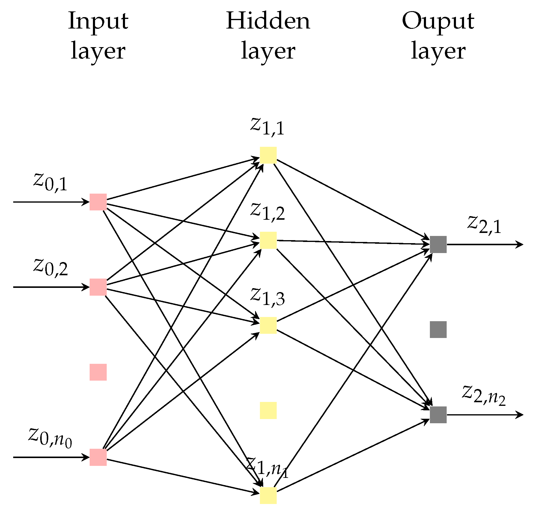
2. Feed forward Neural Networks

A feed-forward neural network (FNN) is an assembly of interconnected processing units referred to as neurons, allocated as input, output and a set of intermediate hidden layers. In this framework, let N k : R d 0 R d k + 1 be an FNN with k hidden layers, with each hidden layer consisting of n j neurons, for j = 1 , 2 , . . . , k . The input and output layers consist of n 0 = d 0 and n k + 1 = d k + 1 neurons, respectively. Each layer except from the input is related to a weight matrix and a bias vector, symbolized as W j and b j , respectively; the sets of these quantities, when considered for all the network layers, define the adjustable parameters of the model. The input vector is written as z 0 R d 0 and the output vector of the j t h layer is written as z j R d j , for j = 1 , 2 , . . . , k + 1 . A schematic representation of a FNN architecture with one hidden layer is portrayed in Figure 1.
The implementation of a network’s layer, j, can be depicted using the following equation:
z j = δ j ( W j z j 1 + b j ) , j { 1 , 2 , . . . , k + 1 }
where δ j ( · ) is a non-linear activation function which is applied layer-wise. Consequently, the implementation of an FNN can be seen as a function mapping inputs z 0 R d 0 to outputs z k + 1 R d k + 1 , using Equation (1).
The activation functions are nonlinear; thus, the minimization of the loss function is a non-convex problem, and consequently can only be solved with non-linear iterative algorithms such as stochastic gradient descent [63] and quasi Newton methods [64]. In the present paper, the FNN method is applied in order to construct the NN that estimate the failure stresses, and the corresponding strains of a shallow foundation in the cohesive soil domain.

3. Numerical Formulation and Material Constitutive Model

Cohesive geomaterials under loading can respond to soil-pore–fluid interaction in fully or partially saturated soil domains. These are referred to as porous media and the physical and mathematical problems that predict their response are called porous media problems. The simulation of a porous medium can be computed using the Biot system of equations. If the load time function is of a low frequency, the Biot problem is redefined at a higher computational cost numerical scheme. The u-p system of equations, which consists of the total set of equations of the soil–fluid momentum balance with the adoption of Darcian flow, coupled with the boundary conditions and the stress–strain material constitutive model, is a numerical simulation which has an augmented numerical stability compared to the corresponding Biot scheme. In this paper, the u-p formulation is adopted because static loads are implied for the soil mass. It should be noted that for a variety of cohesive soils, the u-p scheme is suitable in most of the natural applied forces as depicted in ([65]).
The finite element discretization of the u-p formulation is constructed through classic Galerkin ideas and the following set of equations are obtained [66,67]:
M x ¨ + C x ˙ + K x = f
The extended mass matrix M , stiffness matrix K and damping matrix C are defined as follows:
M = M S 0 0 0
where M S is the conventional mass matrix of the solid skeleton, ρ d is the density of the soil mass, and N u is the shape functions of the displacement field. The mass matrix is computed as follows:
M S = V N u T N u ρ d d v
C = C S 0 Q c T S
where C S stands for the typical damping matrix of the solid skeleton which here is considered as a Rayleigh damping matrix and
K = K S Q c 0 H
In addition, K S represents the standard stiffness matrix of the solid skeleton. B , E are the deformation and elasticity matrices, respectively. The standard stiffness matrix is calculated as follows:
K S = V B T EB d v
The extended matrices consist of the following three parts. The matrix that is used for coupling the system of equations is Q c = V B T m N p d v where m stands for the unity matrix. In the permeability matrix, if k is the matrix of permeability, then H = V ( N p ) T k N p d v . For the saturation matrix, if N P are the shape functions for pore pressure and Q is a function of the bulk moduli of fluid and soil skeleton, then S = V N p 1 Q N p d v . In conclusion, the loading vector divided by the total mixture density b provides an equivalent force vector f S = V ( N p ) T T ( k b ) d v . This numerical algorithm can be calculated using standard implicit or explicit integration schemes such as the Newmark method. Moreover, the load vector and the unknown variables vector are obtained as follows:
f = f S 0 x = u p

4. Numerical Model Implementation

The material constitutive yield function used in this paper is a modified Cam Clay type yield material constitutive model based on the theory of structured soils and critical state theory. Hereinafter, the stresses defined are the effective stresses in the solid skeleton and not in the pores. The yield function consists of mathematical equations for two surfaces, namely the plastic yield envelope (PYE) for interpreting the elastic region and the bond strength envelope (BSE), which defines the allowable places in which PYE may be present ([62,68,69,70,71]). BSE’s magnitude is influenced by the structure of the cohesive soil microtiles. When a stress tensor is situated in the BSE boundary, the degradation rate of the clayey soil structure is maximized. The envelopes are in an ellipsoidal shape and subsequently may have one and only one common point.
The general mathematical representation of an envelope is denoted as follows:
f g ( p h , s , p L , s L , a ) = 1 c 2 ( s s L ) : ( s s L ) + ( p h p L ) 2 ( ξ a ) 2 = 0
In Equation (9) for σ , there is a hydrostatic counterpart p h and a deviatoric counterpart s , while the center of the ellipse L consists of a hydrostatic counterpart p L and a deviatoric counterpart s L . In addition, a is the half-size of the greater diameter of BSE and a ratio of reduction in the PYE in relation to BSE ξ is incorporated. If s L = 0 , p L = a it is concluded that ξ = 1 and consequently BSE is:
f g ( p h , s , p L , s L , a ) = F ( p h , s , a ) = 1 c 2 s : s + ( p h a ) 2 a 2 = 0
However, when the hydrostatic term differs from a and the deviatoric term of the center of the ellipse differs from zero, then the plastic yield envelope has a more general from, as follows:
f g ( p h , s , p L , s L , a ) = f p ( p h , s , p L , s L , a )
The elastic behaviour of the soil is assumed to be isotropically poroelastic. Since the Poisson ratio is constant, the modulus of volumetric deformation, analogous to the shear deformation modulus, can be obtained as follows:
K b u l k = ν p h κ
ν denotes the specific volume of the soil.
This groundwork is implemented in the present article in order to obtain the maximum reliability of the derived NN. Material constitutive modelling coupled with the stochastic finite element method augment the accuracy of the uncertainty quantification and the statistical moments derivation; subsequently, the NN accuracy improves with an alleviated computational cost in terms of the training epochs.

5. Numerical Modeling Results and NN Model Development

5.1. Description of the Numerical Simulations

The numerical simulation formulation is used in porous problems, as depicted in Figure 2 and Figure 3 and follow Equation (2). The output variables under discussion are the stresses and strains at failure of a shallow foundation, which is represented by the equivalent loads of the points A, B, C, and D of Figure 2 and Figure 3. The aforementioned stresses and strains are both related to the volumetric part and the deviatoric part. The modelling of the foundation is performed solely by entering the equivalent nodal loads of each linear distribution of the stresses that apply to a given triad of axial force, and its moments. The loading conditions consist of the nodal values q 1 q 4 at points B, C, A, and D, respectively. The distribution of the equivalent loads is along the area ABCD, which has dimensions of (1 × 1 m 2 ). The triad of eccentricities coupled with the obliquity of the footing load ( e x = M x N , e y = M y N , θ q ) may be considered with the following triads: ( 0 , 0 , 90 ) , ( h 12 , 0 , 90 ) , ( h 6 , 0 , 90 ) , ( h 3 , 0 , 90 ) , ( h 6 , h 6 , 90 ) , ( h 3 , h 6 , 90 ) , ( h 3 , h 3 , 90 ) , ( 0 , 0 , 0 ) , ( 0 , 0 , 30 ) , ( 0 , 0 , 45 ) , ( 0 , 0 , 60 ) , where h is the corresponding length of the footing settlement for each non-central load. The finite element mesh is defined by eight node hexahedral finite elements with linear shape functions for displacements and pore pressures, which provide quantitatively accurate results ([72,73]). The finite element hexahedral mesh total lengths in the X, Y, Z global dimensions in meters are: l x = 5 , l y = 5 , l z = 4 , which consists of a total of 100 elements. The mesh adopted was compared to finer meshes and it was found that the divergence in the calculated displacements is in the acceptable error range of 5%. The geostatic stress situation is incorporated in the numerical system as the initial conditions with the equations σ v = γ z , σ x = σ y = 100 kPa. This hypothesis was made while taking into account that an overstressed clay is simulated, and a corresponding modulus of volumetric deformation in the vicinity of 20 MPa should be assumed. The overall time of the analysis is one day, which was selected in order to respond in a quasi static manner and the time step for each simulation is dt = 0.001 d. The time history of the displacement was plotted; here, the quasi static conditions of the soil domain were verified. The equations applied to boundary surfaces are as follows: u x ( z = h ) = u y ( z = h ) = u z ( z = h ) = 0 and the lateral boundary surfaces do not have constraints. The input material uncertainty consists of the material variables, the compressibility factor κ , the critical state line inclination c, and the permeability factor.
The validity and the reliability of the proposed methodology are analyzed hereinafter. The validity of the numerical simulation programming package which is the Open Source numerical finite element simulation code of National Technical University of Athens, named MSolve, is presented in Figure 4, where an arbitrarily chosen deterministic analysis has been compared to the solution of the commercial code Ansys. The response over time of the numerical structure and the values diverge with a percentage rate of smaller than 5%; consequently, the reliability of the finite element simulations is confirmed. Moreover, in the previous scientific publications of the authors [28,29,30,31], the accuracy of the Monte Carlo simulations in predicting the first two statistical moments has been presented. For clarity, a convergence analysis for the prediction of mean value and standard deviation of the Monte Carlo simulations for an arbitrarily chosen analysis is portrayed in Figure 5, where it is confirmed that the 100 samples taken are sufficient for estimating the monitored output variables’ statistical properties.
The compressibility factor κ , is considered to have spatial distribution with respect to depth as linear ( κ L ), or constant ( κ C ). In the κ L spatial distribution, κ z = 0 = 0.008686 and the ratio R follow the truncated normal distribution with R = κ z = m a x κ z = 0 . The linear relation of the compressibility factor to depth is adopted as a common conjecture of this material parameter equation. This depicts the fact that for in situ conditions when the depth is augmented, κ is reduced; thus, the bulk modulus is augmented. In addition, the value for κ at the top is adopted as deterministic in this paper since in the upper place of the soil domain it is convenient to evaluate the material parameter; subsequently, it can be assumed as non stochastic. The ratio has mean value μ R = 0.469 and the coefficient of variation (CoV) is 0.25; therefore, κ z = m a x , m e a n = 0.004074 . These values are considered in order for the mean stiffness of the soil to possess a shear velocity of 200 m s . It is found that the bulk and the shear moduli are proportional, since the Poisson ratio is constant. So, κ is directly influenced by the shear velocity. If κ is constant in the whole soil mass, the mean value of κ is κ μ = 0.004074 and the CoV is 0.25.
The critical state inclination c is considered constant across the whole soil mass. The value is assumed either as following a random variable or as deterministic. If a random variable case is assumed c R , the friction angle ϕ 0 follows the truncated normal distribution PDF with the mean value of μ ϕ = 23 and the standard deviation of σ ϕ = 2 . which provides values for ϕ 0 using the Latin Hypercube Sampling method. The random vector of ϕ 0 consists of values related to the majority of natural clays as pointed out in ([62]). The ϕ 0 random discrete array elements are collected by following the standard normal distribution sample selection with the use of Latin Hypercube Sampling; as a result, they are altered to the truncated normal probability density function. Consequently, c is computed using the relation c = 2 3 6 s i n ( ϕ 0 ) 3 s i n ( ϕ 0 ) . If c is assumed to be deterministic, it is depicted as c D , c = 0.7336 for friction angle μ ϕ = 23 .
The permeability k, is assumed constant throughout the soil domain. The exact value may be assumed as following a random variable or as deterministic. If a random variable is the hypothesis for k R , the mean value is μ k = 10 8 and the CoV is C o V k = 0.25 . If the deterministic distribution k D is used, k = 10 8 .
Two types of analyses are conducted. The solid analysis, where the fluid–pore pressure is negligible and the porous analyses, where the soil-pore–fluid interaction is taken into account. The solid analyses conducted, denoted with ( S ), are depicted in Table 1, representing a constant (C) or Linear (L) relation for κ and random variable (R) or deterministic (D) assumptions for c. The porous analyses conducted are portrayed in Table 2, including random field (RF), linear (L), and constant (C) relations for κ . Random variable case (R), random field spatial distribution (RF) and the deterministic (D) case for c are represented. Random field relation (RF), random variable case (R) and deterministic cases (D) for k are shown. Alongside the simplification of the Monte Carlo simulation, an abbreviation for the neural network is also introduced.
In stochastic processes, the mean values are as follows: κ m e a n = 0.008686 , c m e a n = 0.7336 and k m e a n = 10 8 m 3 s M g r following the propositions of ([65,67,74]). The standard deviations adopted are: σ κ = 0.25 κ m e a n , σ ϕ = 2 and σ k = 0.25 k m e a n . The exponential autocorrelation function C h = e | Δ x | b is used in all stochastic relations. Correlation length is selected with three possible values, namely b = 2 m ( k R F 2 ), b = 4 m ( k R F 4 ), and b = 8 m ( k R F 8 ). The spatial distributions for κ , κ L , and κ C , are coupled with the random variable distributions for all material variables commensurate to a random variable case simulation. For c, a constant deterministic analysis is implemented. The random field (RF) processes commensurate to the Karhunen Loeve series expansion method and realizations of the spatial stochastic process are formulated through the aforementioned series discrete equation with the implementation of the exponential autocovariance function. A group of random variables ξ that follow the standard normal distribution were obtained with the LHS importance sampling method. The eigenvalues and the eigenfunctions of the autocovariance function C h are provided in closed form equations since the integrodifferential Fredholm eigenproblem has an analytical solution for the exponential formulation of C h . A schematic representation of the random field functions adopted in this work is portrayed in Figure 6. The number of hidden layers used in the analyses is 8. The selection of the hidden layers was performed by choosing 1 layer and performing the FNN construction. Then, by increasing the hidden layers by 1 the average quality of the results was checked. After 8 hidden layers, no better results were obtained; subsequently, the number of hidden layers chosen was 8.
The loads are static and the time of the analyses and the time step were chosen in order to acquire a static response of the soil mass, while eight Fredholm eigenfunctions are implemented. Failure is defined when the first Gaussian Point responds in a softening way, which means that H < 0 where H is the plastic hardening modulus. Each Monte Carlo simulation was adopted for 100 samples collected with the Latin Hypercube Sampling method. The number of the samples was proven adequate in acquiring convergence for the mean value and standard deviation of the output displacements as is shown in the previous scientific publications of the authors. For an arbitrarily chosen simulation, 1000 samples have been collected and calculated for the convergence in comparison to the statistical identities for 100 deterministic subsimulations. The relative error is at most 5 % ; as a result, 100 samples are sufficient for estimating the mean value and standard deviation of the monitored variables in discussion. It should be noted that the cross correlation in all material variables is ignored; thus, the correlation matrix is a diagonal matrix.
In the Monte Carlo simulations analyzed in this section, the FNN procedure described in Section 2 is implemented in order to acquire NNs that predict the failure volumetric stress p v o l , the failure deviatoric equivalent Von Mises stress q d e v , the failure volumetric strain ϵ v o l , and the failure deviatoric equivalent Von Mises strain ϵ d e v . The training was performed in order to minimize the error. Each Monte Carlo simulation provides a distinct set of NNs, and four distinct NNs for each of the monitored output variables is defined. This was performed for both non-porous and porous analyses. The accumulation of the NNs portrays not only the estimation of the aforementioned output variables but also depicts the influence of the assumed spatial variability of the material variables and indicates the qualitative effect of each material variable’s uncertainty to each output variable variability.

5.2. Presentation of the Results-Discussion

The results are depicted in this section. In Table 3, Table 4, Table 5 and Table 6, the convergence study of the neural networks (NN) assimilated from the Monte Carlo simulations in this section is presented, where the L 2 error of each NN is provided. It should be noted that this error is at most in the order of magnitude of 10 2 , indicating the high reliability of the neural network models. Then, the two critical neural networks for porous analyses that predict the most unfavourable values for the volumetric part of the failure stress p v o l , the deviatoric component of the stress q d e v , as well as the corresponding parts of the strain at failure of the footing settlement and the two neural networks for non porous analyses, are portrayed in Figure 7, Figure 8, Figure 9, Figure 10, Figure 11, Figure 12, Figure 13 and Figure 14 with a set of five subfigures each. Each set of subfigures consists of the 3D representation of the NN, the convergence diagram of Loss in relation to the epochs required to train the NN, and the projection of the NN to the input axis x, the eccentricity e x , the input axis y, the eccentricity e y , the input axis z, and the obliquity angle in relation to the horizontal direction θ q . Each neural network illustrated is formed with points that are the mean values of each Monte Carlo Simulation. In the supplementary material, the corresponding estimations of NNs for the rest of the output variables for each unfavourable value are presented. For example, for an NN that is critical for p v o l , the estimations for q d e v , e v o l , e d e v are portrayed in the Supplementary Material.
An analysis of the convergence study indicates that the largest number of epochs is 493,000, which provide an L 2 error of 6.06 × 10 6 . In addition, the largest error is 6.90 × 10 3 with 138,200 epochs. Taking this into consideration alongside the literature related to other physical problems for sciences and engineering [56], it can be deducted that the aforementioned algorithm is suitable for the nature of the problem analyzed. Subsequently, this algorithm is not only easy to implement for training and construction; it is also useful for enriching the model with more data obtained either in situ or computationally. In future, we aim to enrich this high fidelity model with in situ measurement data and investigate the influence of adding such data in the estimation of the footing settlement failure under cohesive geomaterial.
From the data-obtaining procedure and the neural network formulation, useful conclusions can be made. Hereinafter, the critical values of each NN will be given with the input values that lead to the mentioned unfavourable situations. In addition, the other output values estimated once a critical value occurs will be depicted and discussed. Through this study, a comparison scheme will be provided in order to define the most unfavourable situations for the shallow foundation static loading to a stochastic variable soil domain which consists of cohesive geomaterial. This analysis is also quantitatively reliable due to the high fidelity of the material constitutive model and the high accuracy of the neural network method formulation.
NN number 9, which is the Monte Carlo simulation of P - κ R F - c R F - k R F 2 9 , is found to have the most unfavourable values, i.e., the smallest values, for p v o l and q d e v . For p v o l , the critical value is 57.67 kPa, for input triad ( e x , e y , θ ) = (0, 0, 0) with the triad of the rest of the output values estimated to be ( q d e v , e v o l , e d e v ) = (104,879,13,166%,16,631%). For q d e v , the unfavourable value is 103.44 kPa, for input vector ( e x , e y , θ ) = (0, 0, 30 ) with the vector of the remaining output variables predicted as ( p v o l , e v o l , e d e v ) = (59,668,12,583%,14,406%). Consequently, the situation of pure shear load is the worst for the volumetric stresses and the rest of the estimated variables can be described as moderate for stresses and large for strains. Moreover, a central and small oblique load in relation to the horizontal direction is the critical situation for the deviatoric stress and the remaining variables can be described as moderate for stresses and large for strains.
NN number 10, which is the Monte Carlo simulation of P - κ R F - c R F - k R F 4 10 , is found to have the most critical values, i.e., the largest ones, for e v o l and e d e v . For e v o l , the unfavourable value is 14,546%, for the input vector it is ( e x , e y , θ ) = (0, 0, 0), with the vector of the remaining output variables predicted as ( p v o l , q d e v , e d e v ) = (57,923,103,22,18,249%). For e d e v , the critical value is 20,788%, for the input triad it is ( e x , e y , θ ) = (0,0, 90 ) with the triad of the rest monitored variables estimated to be ( p v o l , q d e v , e v o l ) = (654,27,1143,30,12,717%). Subsequently, the situation of pure shear load is the worst for the volumetric strains and the rest of the predicted variables can be portrayed as moderate for stresses and large for strains. In addition, the central and vertical load is the critical situation for the deviatoric stress and the remaining monitored variables can be portrayed as large for stresses and large for strains.
NN d3, which is Monte Carlo simulation S - κ C - c R , is proven to have the most critical values, i.e., the smallest values, for p v o l and q d e v and the largest values for e v o l . For p v o l , the critical value is 59.71 kPa, for the input triad it is ( e x , e y , θ ) = (0, 0, 0) with the triad of the rest output values estimated to be ( q d e v , e v o l , e d e v ) = (99,186,14,418%,16,094%). For q d e v , the unfavourable value is 82,391 kPa, for the input vector it is ( e x , e y , θ )=(0, 0, 30 ), with the vector of the remaining output variables predicted to be ( p v o l , e v o l , e d e v ) = (62,795,16,602%,15,915%). For e v o l , the unfavourable value is 16,603%, for input vector it is ( e x , e y , θ ) = (0, 0, 30 ) with the vector of the remaining output variables predicted to be ( p v o l , q d e v , e d e v ) = (62,795,82,391,15,915%). Consequently, the situation of pure shear load is the worst for the volumetric stresses and the rest of the estimates variables can be described as moderate for stresses and large for strains. Moreover, the central and small oblique load in relation to the horizontal direction is the critical situation for the deviatoric counterpart of stresses and the strain field in both components, and the estimated monitored variables can be portrayed as moderate for stresses and large for strains.
NN d4, which ties in with Monte Carlo simulation S - κ C - c D , is proven to have the most unfavourable values, i.e., the largest values, for e d e v . For e d e v , the critical value is 19,954%, for the input triad it is ( e x , e y , θ ) = ( h 3 , h 3 , 90 ) with the triad of the rest monitored variables estimated to be ( p v o l , q d e v , e v o l ) = (593,789,945,429,10,756%). Consequently, the situation of high eccentric vertical load is critical for deviatoric counterpart of strains, and the remaining variables estimated can be depicted as moderate for stresses and large for strains.
Taking all the above into account, two general deductions can be made. In porous analyses, the most unfavourable situation for output values p v o l , q d e v , e v o l , e d e v is when the input variability follows the Karhunen Loeve random field representation. When correlation length coincides with the depth of the soil mass (b = 4 m), the strain field at failure is at the largest values and consequently the most unfavourable situation takes place. A reduction in the correlation length appears to be slightly influenced by the prediction of the stress field at failure, while the influence on the strains at failure is more profound. Subsequently, the higher the uncertainty is, with the decrease in the correlation length, the greater the variability of the displacement field and strain field at failure is, while for the strain field the variability is smaller. For non porous analyses, we have the worst case scenario for output values p v o l , q d e v , e v o l , e d e v when constant distribution over depth for κ is adopted. To be more specific, for the stresses field and the volumetric part of strains, more critical values are obtained form the NN that considers the critical state line inclination as a random variable case, while for the deviatoric counterpart of strains a more unfavourable situation is attained from the NN that adopts the critical state line inclination as deterministic. Thus, the influence of c is more evident for the stresses, as expected, and for the volumetric part of the strain field; furthermore, the influence of κ is more profound in the estimation of the deviatoric strain field at failure. The results highlight quantitatively and qualitatively the integration of each material variable variability to the response of the soil mass and are similar to the results of previous studies in terms of predicting the response without new analyses needed. In conclusion, the results can be readily enriched by the assimilation of more computational or experimental data. Consequently, the presented article is of significant importance for the scientific areas of computational geomechanics and uncertainty quantification in engineering.

6. Conclusions

In this work, a set of neural networks for the estimation of the failure of footing settlements and the volumetric and deviatoric stresses and strains of the soil at failure under cohesive soils is presented. The data have been assimilated from precedent numerical analyses of Monte Carlo simulations that predict the failure stresses and strain fields of the shallow foundation under static loading conditions. The material yield function of the stress–strain relation provides a high-reliability model for quantitatively accurate stress–strain and force–displacement behaviour measurements of clayey soils under any force field. Subsequently, the output values of the neural network will be verified. The limitations of the aforementioned methodology include the coarse selection of points in the foundation and the selection of mean values for constructing the NN.
In the convergence analysis, the aforementioned neural networks are formed with a relatively low amount of epochs and the L 2 error is alleviated for the reliability required for geotechnical engineering applications. Less than 500,000 epochs are required for a loss in the vicinity of 10 3 . It is also portrayed that the estimation of the stresses at failure requires a significantly smaller amount of epochs in comparison to the corresponding strain field. Moreover, a smaller error is found for the neural networks of the strain field and largest error is found for the corresponding stress field at failure. This indicates the advantages of the method and shows it can be easily enhanced with computational or experimental data, which is an important area of exploration for future work.
In porous analyses, the most critical situation for the output values is when the input uncertainty follows the Karhunen Loeve random field representation. When the correlation length falls, the prediction of the NN for the strain field at failure increases. For non-porous analyses, the respective values of the monitored variables are in general most unfavourable when constant distribution over depth for κ is assumed. This can be explained with the mean value of the Monte Carlo simulation, which was considered at each data point of the constructed Neural Networks. This follows the previous literature published by the authors. When a deterministic value for critical state line inclination is adopted, the deviatoric counterpart of the strains is estimated with the largest values. When a random variable case for c is implemented, the remaining monitored output variables are estimated with the most critical values.

Supplementary Materials

The following supporting information can be downloaded at: https://www.mdpi.com/article/10.3390/geotechnics2040051/s1, Figure S1: Graphical presentation of the Neural Network that corresponds to Monte Carlo analysis P - κ R F - c R F - k R F 2 9 (NN9) for the estimation of the volumetric component of the strain e v o l . Figure S2: Graphical presentation of the Neural Network that corresponds to Monte Carlo analysis P - κ R F - c R F - k R F 2 9 (NN9) for the estimation of the deviatoric component of the strain e d e v . Figure S3: Graphical presentation of the Neural Network that corresponds to Monte Carlo analysis P - κ R F - c R F - k R F 4 10 (NN10) for the estimation of the volumetric component of the stress p v o l in kPa. Figure S4: Graphical presentation of the Neural Network that corresponds to Monte Carlo analysis P - κ R F - c R F - k R F 4 10 (NN10) for the estimation of the deviatoric component of the stress q d e v in kPa. Figure S5: Graphical presentation of the Neural Network that corresponds to Monte Carlo analysis S - κ L - c R -d3 (NND3) for the estimation of the deviatoric component of the strain e d e v . Figure S6: Graphical presentation of the Neural Network that corresponds to Monte Carlo analysis S - κ L - c D -d4 (NND4) for the estimation of the volumetric component of the stress p v o l in kPa. Figure S7: Graphical presentation of the Neural Network that corresponds to Monte Carlo analysis S - κ L - c D -d4 (NND4) for the estimation of the deviatoric component of the stress q d e v in kPa. Figure S8: Graphical presentation of the Neural Network that corresponds to Monte Carlo analysis S - κ L - c D -d4 (NND4) for the estimation of the volumetric component of the strain e v o l .

Author Contributions

Conceptualization, A.-A.S.; methodology, A.-A.S.; data curation, A.-A.S. and L.P. writing—original draft preparation, A.-A.S.; writing—review and editing, A.-A.S. All authors have read and agreed to the published version of the manuscript.

Funding

This research has been funded by the European Research Council Advanced Grant DComex, Data driven computational mechanics at exascale (Project Number 956201) and the Greek research project Materialize, Integrated cloud platform for the standardization and design of materials and products of high performance (MIS 5129436) of the Hellenic Republic and the European Union. The APC was funded by MDPI.

Data Availability Statement

The data that support the findings of this study are not openly available for simplicity and are available from the corresponding author upon reasonable request via the email address provided. Open source code MSolve in programming Language C#. Information can be found at the following link: http://mgroup.ntua.gr/ (accessed on 1 November 2022).

Acknowledgments

This research has been supported by the European Research Council Advanced Grant DComex, Data driven computational mechanics at exascale (Project Number 956201) and the Greek research project Materialize, Integrated cloud platform for the standardization and design of materials and products of high performance (MIS 5129436) of the Hellenic Republic and the European Union.

Conflicts of Interest

The authors declare no conflict of interest.

Nomenclature

The following symbols are used in this manuscript:
N f Friction variables
N q Friction variable indicating the influence of possible vertical load in the lateral
direction of the foundation
N c Friction variable indicating the influence of the cohesion of the soil
N γ Friction variable indicating the influence of the settlement dimensions
alongside the total weight of the soil
S f Shape variables
S q Shape variable indicating the influence of possible vertical load in the lateral
direction of the foundation
S c Shape variable indicating the influence of the cohesion of the soil
S γ Shape variable indicating the influence of the settlement dimensions
alongside the total weight of the soil
κ Compressibility factor
cCritical state line inclination
kPermeability in units m 3 s M g r
ϕ 0 Friction angle
M Total mass matrix
C Total damping matrix
K Total stiffness matrix
M s Solid skeleton mass matrix
ρ d Density of the soil
B Deformation matrix
E Elasticity matrix
C s Solid skeleton damping matrix
K s Solid skeleton stiffness matrix
m Unity matrix
b Loading vector
k Matrix of permeability in units m 3 s M g r
N P Shape functions for pore pressure
N u Shape functions for displacements
S Saturation matrix
Q c Coupling matrix
H Permeability matrix
f S Equivalent forces due to external loading
QVariable for combining the influence of bulk moduli of fluid and solid skeleton in
porous problems
σ Total stress tensor
s Deviatoric component of the stress tensor
p h Hydrostatic component of the stress tensor
aHalfsize of the Bond Strength Envelope
s L Deviatoric component of the stress point of the center of the Plastic Yield Envelope
p L Hydrostatic component of the stress point of the center of the Plastic Yield Envelope
ξ Similarity factor between the Plastic Yield Envelope and Bond Strength Envelope
f g Generalized elliptic envelope
f p Plastic Yield Envelope (PYE)
FBond Strength Envelope (BSE)
ν Specific volume of the soil
qVon Mises stress
eDeviatoric strain measure
ϵ dev Deviatoric component of the strain tensor
fRandom function
f i Value of the random function at nodal points
N i Shape functions
N 0 Total number of shape functions
h 1 Truncated normal PDF
ϕ ( x ) Standard normal PDF
Φ ( x ) Standard normal CDF
σ d Standard deviation of the random variable before truncation
A, B, X 0 Normalized coordinates of the subspace of the truncated PDF
limits and x
H 1 ( x , ω ) Karhunen Loeve random field
N s Number of subintervals in the Latin Hypercube Sampling
μ ( x ) Mean value of the random field
X ( x 1 , x 2 , . . . x n ) Random vector created with Latin Hypercube Sampling
M e , λ i , ϕ i Total number of eigenvalues λ i and eigenfunctions
ϕ i , respectively
bCorrelation length
C O V ( ξ i , ξ j ) Covariance function
λ * Load factor causing failure of the body at exactly the time that ends
the rampload function
TTime at which the rampload function ends
T p Symmetrization factor of the stochastic process
λ n Trial load factor of step n causing failure
t n Time of failure at the generalized load factor λ n
λ m a x n o f a i l u r e Maximum trial load factor which causes safety
λ 1 , f a i l Initial trial load factor causing failure
λ 1 , n o f a i l u r e Initial trial load factor which causes safety
q 1 q 4 Equivalent forces of the shallow foundation
e = M N Eccentricity
l x l y l z Dimensions of the total finite element mesh
σ v , σ x , σ y Geostatic stresses in vertical direction and directions x and y, respectively
λ Inclination of isotropic compression line for the respective normally
consolidated clay
a i n i t i a l Initial halfsize of the ellipse
a r e s i d u a l Residual halfsize of the ellipse
OCROverconsolidation ratio
GShear modulus
K b u l k Bulk modulus
γ Specific weight
ν 0 Initial specific volume of the soil
u x Displacement vector in direction x
κ z = 0 Compressibility factor at depth=0
κ z = m a x Compressibility factor at maximum depth
R = κ z = m a x κ z = 0 Ratio of the compressibility factors measured at depth=0 and at maximum depth
μ R Mean value of ratio R
κ z = m a x , m e a n Compressibility factor at maximum depth when the ratio R has its mean value
κ L Linear distribution over depth for the compressibility factor
κ C Constant distribution over depth for the compressibility factor
κ μ Mean value of κ
c R Random variable case for the critical state line inclination
c D Deterministic case for the critical state line inclination
μ ϕ Mean value of the friction angle
σ ϕ Standard deviation of the friction angle
μ k Mean value of the permeability
C o V k Coefficient of variation of the friction angle
κ m e a n Mean value of the compressibility factor in the random field representation
c m e a n Mean value of the critical state line inclination in the random field representation
k m e a n Mean value of the permeability in the random field representation
σ κ Standard deviation of the compressibility factor in the random field
representation
σ ϕ Standard deviation of the critical state line inclination in the random field
representation
σ k Standard deviation of the permeability in the random field representation
μ ν Mean values of the results
σ δ Coefficient of variation of the results
MMaximum values of the results
μ Minimum values of the results
NTotal settlement force
u x Horizontal displacement at failure
u y Vertical displacement at failure
p v o l Volumetric stress at failure
q d e v Von Mises stress at failure
e v o l Volumetric strain at failure
e d e v Deviatoric strain at failure
R v o l Percentage plastic volumetric strains at failure
R d e v Percentage plastic deviatoric strains at failure

References

  1. Terzaghi, K.V. Theoretical Soil Mechanics; Wiley and Sons: Hoboken, NJ, USA, 1966. [Google Scholar]
  2. Michalowski, R.L. An Estimate of the Influence of Soil Weight on Bearing Capacity Using Limit Analysis. Soils Found. 1997, 37, 57–64. [Google Scholar] [CrossRef] [PubMed] [Green Version]
  3. Michalowski, R.L. Upper-bound load estimates on square and rectangular footings. Geotechnique 2001, 51, 787–798. [Google Scholar] [CrossRef]
  4. Martin, C. Exact bearing capacity calculations using the method of characteristics. In Proceedings of the 11th International Conference IACMAG, Graz, Austria, 19–24 June 2005. [Google Scholar]
  5. Rao, P.; Liu, Y.; Cui, J. Bearing capacity of strip footings on two-layered clay under combined loading. Comput. Geotech. 2015, 69, 210–218. [Google Scholar] [CrossRef]
  6. Zafeirakos, A.; Gerolymos, N. Bearing strength surface for bridge caisson foundations in frictional soil under combined loading. Acta Geotech. 2016, 11, 1189–1208. [Google Scholar] [CrossRef]
  7. Zhou, H.; Zheng, G.; Yin, X.; Jia, R.; Yang, X. The bearing capacity and failure mechanism of a vertically loaded strip footing placed on the top of slopes. Comput. Geotech. 2018, 94, 12–21. [Google Scholar] [CrossRef]
  8. Naderi, E.; Asakereh, A.; Dehghani, M. Bearing Capacity of Strip Footing on Clay Slope Reinforced with Stone Columns. Arab. J. Sci. Eng. 2018, 43, 5559–5572. [Google Scholar] [CrossRef]
  9. Sultana, P.; Dey, A.K. Estimation of Ultimate Bearing Capacity of Footings on Soft Clay from Plate Load Test Data Considering Variability. Indian Geotech. J. 2019, 49, 170–183. [Google Scholar] [CrossRef]
  10. Papadopoulou, K.; Gazetas, G. Shape Effects on Bearing Capacity of Footings on Two-Layered Clay. Geotech. Geol. Eng. 2020, 38, 1347–1370. [Google Scholar] [CrossRef]
  11. Fu, D.; Zhang, Y.; Yan, Y. Bearing capacity of a side-rounded suction caisson foundation under general loading in clay. Comput. Geotech. 2020, 123, 103543. [Google Scholar] [CrossRef]
  12. Li, S.; Yu, J.; Huang, M.; Leung, G. Upper bound analysis of rectangular surface footings on clay with linearly increasing strength. Comput. Geotech. 2021, 129, 103896. [Google Scholar] [CrossRef]
  13. Karhunen, K. Uber lineare Methoden in der Wahrscheinlichkeitsrechnung. Ann. Acad. Sci. Fenn. 1947, 37, 1–79. [Google Scholar]
  14. Ghanem, R.; Spanos, D. Stochastic Finite Elements: A Spectral Approach; Springer: Berlin/Heidelberg, Germany, 1991; Volume 1, pp. 1–214. [Google Scholar] [CrossRef]
  15. Papadrakakis, M.; Papadopoulos, V. Robust and efficient methods for the stochastic finite element analysis using Monte Carlo simulation. Comput. Methods Appl. Mech. Eng. 1996, 134, 325–340. [Google Scholar] [CrossRef]
  16. Matthies, H.G.; Brenner, C.E.; Butcher, G.; Soares, C.G. Uncertainties in probabilistic numerical analysis of structures and solids- Stochastic finite elements. Struct. Saf. 1997, 19, 283–336. [Google Scholar] [CrossRef]
  17. Assimaki, D.; Pecker, A.; Popescu, R.; Prevost, J. Effects of spatial variabilty of soil properties on surface ground motion. J. Earthq. Eng. 2003, 7, 1–44. [Google Scholar] [CrossRef]
  18. Popescu, R.; Deodatis, G.; Nobahar, A. Effects of random heterogeneity of soil properties on bearing capacity. Probabilistic Eng. Mech. 2005, 20, 324–341. [Google Scholar] [CrossRef]
  19. Sett, K.; Jeremic, B. Probabilistic elasto-plasticity: Solution and verification in 1D. Acta Geotech. 2007, 2, 211–220. [Google Scholar] [CrossRef]
  20. Meftah, F.; Dal-Pont, S.; Schrefler, B.A. A three-dimensional staggered finite element approach for random parametric modeling of thermo-hygral coupled phenomena in porous media. Int. J. Numer. Anal. Methods Geomech. 2012, 36, 574–596. [Google Scholar] [CrossRef]
  21. Li, D.Q.; Qi, X.H.; Cao, Z.J.; Tang, X.S.; Zhou, W.; Phoon, K.K.; Zhou, C.B. Reliability analysis of strip footing considering spatially variable undrained shear strength that linearly increases with depth. Soils Found. 2015, 55, 866–880. [Google Scholar] [CrossRef] [Green Version]
  22. Liu, W.; Sun, Q.; Miao, H.; Li, J. Nonlinear stochastic seismic analysis of buried pipeline systems. Soil Dyn. Earthq. Eng. 2015, 74, 69–78. [Google Scholar] [CrossRef]
  23. Ali, A.; Lyamin, A.; Huang, J.; Li, J.; Cassidy, M.; Sloan, S. Probabilistic stability assessment using adaptive limit analysis and random fields. Acta Geotech. 2017, 12, 937–948. [Google Scholar] [CrossRef]
  24. Brantson, E.T.; Ju, B.; Wu, D.; Gyan, P.S. Stochastic porous media modeling and high-resolution schemes for numerical simulation of subsurface immiscible fluid flow transport. Acta Geophys. 2018, 66, 243–266. [Google Scholar] [CrossRef]
  25. Chwała, M. Undrained bearing capacity of spatially random soil for rectangular footings. Soils Found. 2019, 59, 1508–1521. [Google Scholar] [CrossRef]
  26. Olsson, A.; Sandberg, G.; Dahlblom, O. On Latin hypercube sampling for structural reliability analysis. Struct. Saf. 2003, 25, 47–68. [Google Scholar] [CrossRef]
  27. Simoes, J.; Neves, L.; Antao, A.; Guerra, N. Reliability assessment of shallow foundations on undrained soils considering soil spatial variability. Comput. Geotech. 2020, 119, 103369. [Google Scholar] [CrossRef]
  28. Savvides, A.; Papadrakakis, M. A computational study on the uncertainty quantification of failure of clays with a modified Cam-Clay yield criterion. Springer Nat. Appl. Sci. 2021, 3, 659. [Google Scholar] [CrossRef]
  29. Savvides, A.; Papadrakakis, M. Probabilistic Failure Estimation of an Oblique Loaded Footing Settlement on Cohesive Geomaterials with a Modified Cam Clay Material Yield Function. Geotechnics 2021, 1, 347–384. [Google Scholar] [CrossRef]
  30. Savvides, A.; Papadrakakis, M. Uncertainty Quantification of Failure of Shallow Foundation on Clayey Soils with a Modified Cam-Clay Yield Criterion and Stochastic FEM. Geotechnics 2022, 2, 348–384. [Google Scholar] [CrossRef]
  31. Savvides, A. Stochastic Failure of a Double Eccentricity Footing Settlement on Cohesive Soils with a Modified Cam Clay Yield Surface. Transp. Porous Media 2022, 141, 499–560. [Google Scholar] [CrossRef]
  32. Raissi, M.; Perdikaris, P.; Karniadakis, G.E. Physics-informed neural networks: A deep learning framework for solving forward and inverse problems involving nonlinear partial differential equations. J. Comput. Phys. 2019, 378, 686–707. [Google Scholar] [CrossRef]
  33. Misyris, G.S.; Venzke, A.; Chatzivasileiadis, S. Physics-Informed Neural Networks for Power Systems. arXiv 2020, arXiv:1911.03737. [Google Scholar]
  34. Desai, S.; Mattheakis, M.; Joy, H.; Protopapas, P.; Roberts, S. One-Shot Transfer Learning of Physics-Informed Neural Networks. arXiv 2021, arXiv:2110.11286. [Google Scholar]
  35. Ramabathiran, A.A.; Ramachandran, P. SPINN: Sparse, Physics-based, and partially Interpretable Neural Networks for PDEs. arXiv 2021, arXiv:2102.13037. [Google Scholar] [CrossRef]
  36. Leung, W.T.; Lin, G.; Zhang, Z. Nh-pinn: Neural homogenization based physics-informed neural network for multiscale problems. arXiv 2021, arXiv:2108.12942. [Google Scholar] [CrossRef]
  37. Abadi, M.; Agarwal, A.; Barham, P.; Brevdo, E.; Chen, Z.; Citro, C.; Corrado, G.S.; Davis, A.; Dean, J.; Devin, M.; et al. TensorFlow: Large-Scale Machine Learning on Heterogeneous Distributed Systems. arXiv 2015, arXiv:1603.04467. [Google Scholar]
  38. Paszke, A.; Gross, S.; Massa, F.; Lerer, A.; Bradbury, J.; Chanan, G.; Killeen, T.; Lin, Z.; Gimelshein, N.; Antiga, L.; et al. PyTorch: An Imperative Style, High-Performance Deep Learning Library. In Proceedings of the Advances in Neural Information Processing Systems 32 (NeurIPS 2019): Annual Conference on Neural Information Processing Systems 2019, Vancouver, BC, Canada, 8–14 December 2019. [Google Scholar]
  39. Kharazmi, E.; Zhang, Z.; Karniadakis, G.E. hp-VPINNs: Variational physics-informed neural networks with domain decomposition. Comput. Methods Appl. Mech. Eng. 2021, 374, 113547. [Google Scholar] [CrossRef]
  40. Meng, X.; Li, Z.; Zhang, D.; Karniadakis, G.E. PPINN: Parareal physics-informed neural network for time-dependent PDEs. Comput. Methods Appl. Mech. Eng. 2020, 370, 113250. [Google Scholar] [CrossRef]
  41. Jagtap, A.D.; Karniadakis, G.E. Extended Physics-Informed Neural Networks (XPINNs): A Generalized Space-Time Domain Decomposition Based Deep Learning Framework for Nonlinear Partial Differential Equations. Comput. Phys. 2020, 28, 2002–2041. [Google Scholar] [CrossRef]
  42. Zhou, W.H.; Garg, A.; Garg, A. Study of the volumetric water content based on density, suction and initial water content. Measurement 2016, 94, 531–537. [Google Scholar] [CrossRef]
  43. Zhang, P.; Yin, Z.Y.; Jin, Y.F.; Chan, T.H.T. A novel hybrid surrogate intelligent model for creep index prediction based on particle swarm optimization and random forest. Eng. Geol. 2020, 265, 105328. [Google Scholar] [CrossRef]
  44. Zhang, P.; Yin, Z.Y.; Jin, Y.F.; Chan, T.H.T.; Gao, F.P. Intelligent modelling of clay compressibility using hybrid meta-heuristic and machine learning algorithms. Geosci. Front. 2021, 12, 441–452. [Google Scholar] [CrossRef]
  45. Zhang, N.S.; Zhou, S.L.; Xu, A.; Shuang, Y. Investigation on Performance of Neural Networks Using Quadratic Relative Error Cost Function. IEEE Access 2019, 7, 106642–106652. [Google Scholar] [CrossRef]
  46. Zhang, P.; Qi, C.; Sun, X.; Fang, H.; Huang, Y. Bending behaviors of the in-plane bidirectional functionally graded piezoelectric material plates. Mech. Adv. Mater. Struct. 2020, 29, 1925–1945. [Google Scholar] [CrossRef]
  47. Njock, P.G.A.; Shen, S.L.; Zhou, A.; Lyu, H.M. Evaluation of soil liquefaction using AI technology incorporating a coupled ENN/ t-SNE model. Soil Dyn. Earthq. Eng. 2020, 130, 105988. [Google Scholar] [CrossRef]
  48. Chen, R.P.; Zhang, P.; Kang, X.; Zhong, Z.Q.; Liu, Y.; Wu, H.N. Prediction of maximum surface settlement caused by earth pressure balance (EPB) shield tunneling with ANN methods. Soils Found. 2019, 59, 284–295. [Google Scholar] [CrossRef]
  49. Chen, R.; Zhang, P.; Wu, H.; Wang, Z.; Zhong, Z. Prediction of shield tunneling-induced ground settlement using machine learning techniques. Front. Struct. Civ. Eng. 2019, 13, 1363–1378. [Google Scholar] [CrossRef]
  50. Elbaz, K.; Shen, S.L.; Zhou, A.; Yuan, D.J.; Xu, Y.S. Optimization of EPB Shield Performance with Adaptive Neuro-Fuzzy Inference System and Genetic Algorithm. Appl. Sci. 2019, 9, 780. [Google Scholar] [CrossRef] [Green Version]
  51. Elbaz, K.; Shen, S.L.; Zhou, A.; Yin, Z.; Lyu, H.M. Prediction of Disc Cutter Life During Shield Tunneling with AI via the Incorporation of a Genetic Algorithm into a GMDH-Type Neural Network. Engineering 2021, 7, 238–251. [Google Scholar] [CrossRef]
  52. Zhang, P.; Chen, R.P.; Wu, H.N. Real-time analysis and regulation of EPB shield steering using Random Forest. Autom. Constr. 2019, 106, 102860. [Google Scholar] [CrossRef]
  53. Zhang, P.; Wu, H.N.; Chen, R.P.; Chan, T.H.T. Hybrid meta-heuristic and machine learning algorithms for tunneling-induced settlement prediction: A comparative study. Tunn. Undergr. Space Technol. 2020, 99, 103383. [Google Scholar] [CrossRef]
  54. Huang, F.; Huang, J.; Jiang, S.; Zhou, C. Landslide displacement prediction based on multivariate chaotic model and extreme learning machine. Eng. Geol. 2017, 218, 173–186. [Google Scholar] [CrossRef]
  55. Yang, B.; Lacasse, S.; Liu, Z. Time series analysis and long short-term memory neural network to predict landslide displacement. Landslides 2019, 16, 677–694. [Google Scholar] [CrossRef]
  56. Zhang, P.; Yin, Z.Y.; Zheng, Y.; Gao, F.P. A LSTM surrogate modelling approach for caisson foundations. Ocean. Eng. 2020, 204, 107263. [Google Scholar] [CrossRef]
  57. Liu, Z.; Gilbert, G.; Cepeda, J.M.; Lysdahl, A.O.K.; Piciullo, L.; Hefre, H.; Lacasse, S. Modelling of shallow landslides with machine learning algorithms. Geosci. Front. 2021, 12, 385–393. [Google Scholar] [CrossRef]
  58. Wu, Z.; Wei, R.; Chu, Z.; Liu, Q. Real-time rock mass condition prediction with TBM tunneling big data using a novel rock–machine mutual feedback perception method. J. Rock Mech. Geotech. Eng. 2021, 13, 1311–1325. [Google Scholar] [CrossRef]
  59. Wu, C.; Hong, L.; Wang, L.; Zhangd, R.; Pijushe, S.; Zhang, W. Prediction of wall deflection induced by braced excavation in spatially variable soils via convolutional neural network. Gondwana Res. 2022. [Google Scholar] [CrossRef]
  60. Zhang, W.; Gu, X.; Tang, L.; Yin, Y.; Liu, D.; Zhang, Y. Application of machine learning, deep learning and optimization algorithms in geoengineering and geoscience: Comprehensive review and future challenge. Gondwana Res. 2022, 109, 1–17. [Google Scholar] [CrossRef]
  61. Zhang, N.; Zhang, N.; Zheng, Q.; Xu, Y.S. Real-time prediction of shield moving trajectory during tunnelling using GRU deep neural network. Acta Geotech. 2022, 17, 1167–1182. [Google Scholar] [CrossRef]
  62. Kavvadas, M.; Amorosi, A. A constitutive model for structured soils. Geotechnique 2000, 50, 263–273. [Google Scholar] [CrossRef]
  63. Kingma, D.P.; Ba, J. A method for stochastic optimization. arXiv 2015, arXiv:1412.6980. [Google Scholar]
  64. Fletcher, R. Practical Methods of Optimization; Wiley and Sons: Hoboken, NJ, USA, 1987. [Google Scholar]
  65. Zienkiewicz, O.C.; Chan, A.H.C.; Pastor, M.; Schrefler, B.A.; Shiomi, T. Computational Geomechanics with Special Reference to Earthquake Engineering; Wiley: Chichester, UK, 1999; Volume 1, pp. 17–49. [Google Scholar]
  66. Biot, M.A. General theory of three dimensional consolidation. J. Appl. Phys. 1941, 12, 155–164. [Google Scholar] [CrossRef]
  67. Lewis, R.W.; Schrefler, B.A. The Finite Element Method in the Deformation and Consolidation of Porous Media; Wiley and Sons: Hoboken, NJ, USA, 1988; Volume 1, pp. 1–508. [Google Scholar] [CrossRef]
  68. Borja, R.; Lee, S. Cam-Clay plasticity, Part 1: Implicit integration of elasto-plastic constitutive relations. Comput. Methods Appl. Mech. Eng. 1990, 78, 49–72. [Google Scholar] [CrossRef]
  69. Borja, R. Cam-Clay plasticity, Part 2: Implicit integration of constitutive equation based on a nonlinear elastic stress predictor. Comput. Methods Appl. Mech. Eng. 1991, 88, 225–240. [Google Scholar] [CrossRef]
  70. Kalos, A. Investigation of the nonlinear time-dependent soil behavior. PhD Diss. NTUA 2014, 1, 193–236. [Google Scholar]
  71. Vrakas, A. On the computational applicability of the modified Cam-clay model on the ‘dry’ side. Comput. Geotech. 2018, 94, 214–230. [Google Scholar] [CrossRef]
  72. Melenk, J.M.; Babuska, I. The partition of unity finite element method: Basic theory and applications. Comput. Methods Appl. Mech. Eng. 1996, 139, 289–314. [Google Scholar] [CrossRef] [Green Version]
  73. Szabo, B.; Babuska, I. Intoduction to Finite Element Analysis. Formulation, Verification and Validation; Wiley Series in Computational Mechanics; John Wiley & Sons: Hoboken, NJ, USA, 2011; Volume 1, pp. 1–382. [Google Scholar] [CrossRef]
  74. Stickle, M.M.; Yague, A.; Pastor, M. Free Finite Element Approach for Saturated Porous Media: Consolidation. Math. Probl. Eng. 2016, 2016, 4256079. [Google Scholar] [CrossRef]
Figure 1. A feed-forward Neural Network with one hidden layer.
Geotechnics 02 00051 g001
Figure 2. The soil domain and the loads applied for non oblique loading, where l x = 5 m ,   l y = 5 m , l z = 4 m and q 1 = m a x ( q 1 , q 2 , q 3 , q 4 ) , q 2 = m i n ( q 1 , q 2 , q 3 , q 4 ) . The lines colored in maroon indicate the boundary conditions and the points considered as fixed u x ( z = h ) = u y ( z = h ) = u z ( z = h ) = 0 .
Geotechnics 02 00051 g002
Figure 3. The soil domain and the loads applied for oblique loading, where l x = 5 m ,   l y = 5 m , l z = 4 m and q 1 = m a x ( q 1 , q 2 , q 3 , q 4 ) , q 2 = m i n ( q 1 , q 2 , q 3 , q 4 ) . The lines colored in maroon indicate the boundary conditions and the points considered as fixed u x ( z = h ) = u y ( z = h ) = u z ( z = h ) = 0 .
Geotechnics 02 00051 g003
Figure 4. Validation of the method implemented and the Open Source numerical finite element simulation code MSolve. A randomly chosen deterministic analysis has been compared to the corresponding analysis with Ansys. The results diverge with a rate smaller than 5%; thus, the validity holds.
Geotechnics 02 00051 g004
Figure 5. Convergence of the mean value and the standard deviation of a randomly selected Monte Carlo simulation for the output failure load. The reference value of the percentage difference is the statistical moment in 100 samples.
Geotechnics 02 00051 g005
Figure 6. Schematic representation of the realizations of the random field simulations for the correlation lengths b = 2 m, b = 4 m, b = 8 m.
Geotechnics 02 00051 g006
Figure 7. Graphical presentation of the Neural Network that corresponds to Monte Carlo analysis P - κ R F - c R F - k R F 2 9 (NN9) for the estimation of the volumetric component of the stress p v o l in kPa. (a) 3D representation of the Neural Network. (b) Epochs-Loss diagram. (c) Neural Network representation in the projection to the input axis of e x . (d) Neural Network representation in the projection to the input axis of e y . (e) Neural Network representation in the projection of the input axis of θ .
Geotechnics 02 00051 g007
Figure 8. Graphical presentation of the Neural Network that corresponds to Monte Carlo analysis P - κ R F - c R F - k R F 2 9 (NN9) for the estimation of the deviatoric component of the stress q d e v in kPa. (a) 3D representation of the Neural Network. (b) Epochs-Loss diagram. (c) Neural Network representation in the projection to the input axis of e x . (d) Neural Network representation in the projection to the input axis of e y . (e) Neural Network representation in the projection to the input axis of θ .
Geotechnics 02 00051 g008aGeotechnics 02 00051 g008b
Figure 9. Graphical presentation of the Neural Network that corresponds to Monte Carlo analysis P - κ R F - c R F - k R F 4 10 (NN10) for the estimation of the volumetric component of the strain e v o l . (a) 3D representation of the Neural Network. (b) Epochs-Loss diagram. (c) Neural Network representation in the projection of the input axis of e x . (d) Neural Network representation in the projection to the input axis of e y . (e) Neural Network representation in the projection of the input axis of θ .
Geotechnics 02 00051 g009
Figure 10. Graphical presentation of the Neural Network that corresponds to Monte Carlo analysis P - κ R F - c R F - k R F 4 10 (NN10) for the estimation of the deviatoric component of the strain e d e v . (a) 3D representation of the Neural Network. (b) Epochs-Loss diagram. (c) Neural Network representation in the projection of the input axis of e x . (d) Neural Network representation in the projection of the input axis of e y . (e) Neural Network representation in the projection of the input axis of θ .
Geotechnics 02 00051 g010
Figure 11. Graphical presentation of the Neural Network that corresponds to Monte Carlo analysis S - κ L - c R -d3 (NND3) for the estimation of the volumetric component of the stress p v o l in kPa. (a) 3D representation of the Neural Network. (b) Epochs-Loss diagram. (c) Neural Network representation in the projection of the input axis of e x . (d) Neural Network representation in the projection of the input axis of e y . (e) Neural Network representation in the projection of the input axis of θ .
Geotechnics 02 00051 g011aGeotechnics 02 00051 g011b
Figure 12. Graphical presentation of the Neural Network that corresponds to Monte Carlo analysis S - κ L - c R -d3 (NND3) for the estimation of the deviatoric component of the stress q d e v in kPa. (a) 3D representation of the Neural Network. (b) Epochs-Loss diagram. (c) Neural Network representation in the projection of the input axis of e x . (d) Neural Network representation in the projection of the input axis of e y . (e) Neural Network representation in the projection of the input axis of θ .
Geotechnics 02 00051 g012
Figure 13. Graphical presentation of the Neural Network that corresponds to Monte Carlo analysis S - κ L - c R -d3 (NND3) for the estimation of the volumetric component of the strain e v o l . (a) 3D representation of the Neural Network. (b) Epochs-Loss diagram. (c) Neural Network representation in the projection of the input axis of e x . (d) Neural Network representation in the projection of the input axis of e y . (e) Neural Network representation in the projection of the input axis of θ .
Geotechnics 02 00051 g013
Figure 14. Graphical presentation of the Neural Network that corresponds to Monte Carlo analysis S - κ L - c D -d4 (NND4) for the estimation of the deviatoric component of the strain e d e v . (a) 3D representation of the Neural Network; (b) Epochs-Loss diagram; (c) Neural Network representation in the projection to the input axis of e x ; (d) Neural Network representation in the projection to the input axis of e y ; (e) Neural Network representation in the projection to the input axis of θ .
Geotechnics 02 00051 g014aGeotechnics 02 00051 g014b
Table 1. Non porous (solid) analyses conducted.
κ cAbbreviation-NN Number
LinearRandom S - κ L - c R -d1
LinearDeterministic S - κ L - c D -d2
ConstantRandom S - κ C - c R -d3
ConstantDeterministic S - κ C - c D -d4
Table 2. Porous analyses conducted.
κ ckAbbreviation-NN Number
ConstantRandomDeterministic P - κ C - c R - k D 1
ConstantRandomRandom P - κ C - c R - k R 2
ConstantDeterministicRandom P - κ C - c D - k R 3
ConstantDeterministicDeterministic P - κ C - c D - k D 4
LinearRandomDeterministic P - κ L - c R - k D 5
LinearRandomRandom P - κ L - c R - k R 6
LinearDeterministicRandom P - κ L - c D - k R 7
LinearDeterministicDeterministic P - κ L - c D - k D 8
Random Field, b = 2Random Field, b = 2Random Field, b = 2 P - κ R F - c R F - k R F 2 9
Random Field, b = 4Random Field, b = 4Random Field, b = 4 P - κ R F - c R F - k R F 4 10
Random Field, b = 8Random Field, b = 8Random Field, b = 8 P - κ R F - c R F - k R F 8 11
Table 3. Number of epochs for convergence and the corresponding L 2 loss for Neural Networks for Monte Carlo simulations of porous analyses with deterministic shape functions for the stochastic material variables ( κ considered constant over depth).
NeurNet and Number# of Epochs L 2 Loss
κ C c D k D 4 , p v o l 194 , 000 6.9 × 10 4
κ C c D k D 4 , q d e v 187 , 200 8.89 × 10 8
κ C c D k D 4 , e v o l 90 , 500 4.34 × 10 13
κ C c D k D 4 , e d e v 134 , 700 4.96 × 10 13
κ C c R k D 1 , p v o l 164 , 400 4.36 × 10 7
κ C c R k D 1 , q d e v 198 , 000 1.56 × 10 7
κ C c R k D 1 , e v o l 139 , 700 5.78 × 10 13
κ C c R k D 1 , e d e v 159 , 800 8.02 × 10 12
κ L c D k D 8 , p v o l 125 , 900 4.05 × 10 8
κ L c D k D 8 , q d e v 156 , 100 8.83 × 10 9
κ L c D k D 8 , e v o l 134 , 200 1.19 × 10 6
κ L c D k D 8 , e d e v 20 , 000 1.10 × 10 3
κ L c R k D 5 , p v o l 130,900 1.95 × 10 5
κ L c R k D 5 , q d e v 138,000 7.49 × 10 9
κ L c R k D 5 , e v o l 118 , 200 8.26 × 10 13
κ L c R k D 5 , e d e v 187 , 200 8.11 × 10 4
Table 4. Number of epochs for convergence and the corresponding L 2 loss for Neural Networks for Monte Carlo simulations of porous analyses with deterministic shape functions for the stochastic material variables ( κ considered linear over depth).
NeurNet and Number# of Epochs L 2 Loss
κ C c D k R 3 , p v o l 172 , 500 4.07 × 10 9
κ C c D k R 3 , q d e v 195 , 500 2.51 × 10 4
κ C c D k R 3 , e v o l 84 , 900 7.85 × 10 13
κ C c D k R 3 , e d e v 138 , 700 4.13 × 10 13
κ C c R k R 2 , p v o l 183 , 200 6.90 × 10 3
κ C c R k R 2 , q d e v 165 , 700 4.02 × 10 5
κ C c R k R 2 , e v o l 160 , 500 1.19 × 10 12
κ C c R k R 2 , e d e v 200 , 000 3.43 × 10 10
κ L c D k R 7 , p v o l 171 , 400 2.66 × 10 8
κ L c D k R 7 , q d e v 110 , 300 2.66 × 10 7
κ L c D k R 7 , e v o l 161,400 4.96 × 10 13
κ L c D k R 7 , e d e v 493,000 6.06 × 10 6
κ L c R k R 6 , p v o l 189 , 000 4.70 × 10 8
κ L c R k R 6 , q d e v 187 , 200 8.89 × 10 8
κ L c R k R 6 , e v o l 188 , 100 4.76 × 10 9
κ L c R k R 6 , e d e v 199 , 900 2.17 × 10 4
Table 5. Number of epochs for convergence and the corresponding L 2 loss for Neural Networks for Monte Carlo simulations of porous analyses with stochastic spatial representation for all the stochastic material variables.
NeurNet and Number# of Epochs L 2 Loss
κ R F c R F k R F 2 9 , p v o l 186 , 600 8.27 × 10 8
κ R F c R F k R F 2 9 , q d e v 112 , 600 3.26 × 10 8
κ R F c R F k R F 2 9 , e v o l 141 , 300 1.40 × 10 12
κ R F c R F k R F 2 9 , e d e v 200 , 000 1.19 × 10 3
κ R F c R F k R F 4 10 , p v o l 87 , 700 3.67 × 10 8
κ R F c R F k R F 4 10 , q d e v 171 , 400 6.14 × 10 9
κ R F c R F k R F 4 10 , e v o l 164 , 300 4.13 × 10 13
κ R F c R F k R F 4 10 , e d e v 57 , 600 4.29 × 10 12
κ R F c R F k R F 8 11 , p v o l 116,100 5.09 × 10 9
κ R F c R F k R F 8 11 , q d e v 50,000 7.22 × 10 9
κ R F c R F k R F 8 11 , e v o l 143,300 6.75 × 10 3
κ R F c R F k R F 8 11 , e d e v 65,200 6.61 × 10 13
Table 6. Number of epochs for convergence and the corresponding L 2 loss for Neural Networks for Monte Carlo simulations of non porous medium.
NeurNet# of Epochs L 2 Loss
κ C c D d 4 , p v o l 177 , 800 2.00 × 10 4
κ C c D d 4 , q d e v 137 , 200 9.67 × 10 7
κ C c D d 4 , e v o l 168 , 500 3.48 × 10 7
κ C c D d 4 , e d e v 20 , 000 2.05 × 10 5
κ C c R d 3 , p v o l 110 , 500 5.53 × 10 5
κ C c R d 3 , q d e v 199 , 100 5.61 × 10 3
κ C c R d 3 , e v o l 179 , 900 7.33 × 10 12
κ C c R d 3 , e d e v 200 , 000 4.77 × 10 4
κ L c D d 2 , p v o l 200 , 000 0.60 × 10 3
κ L c D d 2 , q d e v 126 , 400 1.87 × 10 6
κ L c D d 2 , e v o l 200 , 000 1.73 × 10 4
κ L c D d 2 , e d e v 200 , 000 1.07 × 10 5
κ L c R d 1 , p v o l 159,400 1.60 × 10 8
κ L c R d 1 , q d e v 200,000 5.84 × 10 8
κ L c R d 1 , e v o l 200,000 4.62 × 10 5
κ L c R d 1 , e d e v 199,600 3.00 × 10 5
Publisher’s Note: MDPI stays neutral with regard to jurisdictional claims in published maps and institutional affiliations.

