Article

Probabilistic Seismic Risk Analysis of Buried Pipelines Due to Permanent Ground Deformation for Victoria, BC

School of Engineering, Faculty of Applied Science, Okanagan Campus, EME4242-1137 Alumni Ave., Kelowna, BC V1V 1V7, Canada
*
Author to whom correspondence should be addressed.
Geotechnics 2022, 2(3), 731-753; https://doi.org/10.3390/geotechnics2030035
Submission received: 8 July 2022 / Revised: 9 August 2022 / Accepted: 16 August 2022 / Published: 31 August 2022

Abstract

:
Buried continuous pipelines are prone to failure due to permanent ground deformation as a result of fault rupture. Since the failure mode is dependent on a number of factors, a probabilistic approach is necessary to correctly compute the seismic risk. In this study, a novel method to estimate regional seismic risk to buried continuous pipelines is presented. The seismic risk assessment method is thereafter illustrated for buried gas pipelines in the City of Victoria, British Columbia. The illustrated example considers seismic hazard from the Leech River Valley Fault Zone (LRVFZ). The risk assessment approach considers uncertainties of earthquake rupture, soil properties at the site concerned, geometric properties of pipes and operating conditions. Major improvements in this method over existing comparable studies include the use of stochastic earthquake source modeling and analytical Okada solutions to generate regional ground deformation, probabilistically. Previous studies used regression equations to define probabilistic ground deformations along a fault. Secondly, in the current study, experimentally evaluated 3D shell and continuum pipe–soil finite element models were used to compute pipeline responses. Earlier investigations used simple soil spring–beam element pipe models to evaluate the pipeline response. Finally, the current approach uses the multi-fidelity Gaussian process surrogate model to ensure efficiency and limit required computational resources. The developed multi-fidelity Gaussian process surrogate model was successfully cross-validated with high coefficients of determination of 0.92 and 0.96. A fragility curve was generated based on failure criteria from ALA strain limits. The seismic risks of pipeline failure due to compressive buckling and tensile rupture at the given site considered were computed to be 1.5 percent and 0.6 percent in 50 years, respectively.

1. Introduction

Buried continuous pipelines are in use around the world for transporting oil and gas. Identification of vulnerable portions of such buried pipelines infrastructure, under seismic loads, is necessary to prioritize mitigation efforts. In contrast to segmented pipelines, buried continuous pipelines are more prone to failure due to permanent ground deformation rather than seismic wave propagation, as mentioned in [1]. As opposed to other types of infrastructure, where the primary form of mitigation against fault rupture hazard has been avoidance, buried pipelines can not avoid seismically active zones and must traverse through these high risk zones. The physical process of buried continuous pipeline undergoing surface rupture displacements is quite a complicated one. The failure mode and generated strains depend on the nature of faulting, ground deformation magnitude, the pipeline’s material and geometric properties, operating conditions in the pipe and soil conditions. Such a problem calls for probabilistic approaches to compute the seismic risk. Most of the analytical and numerical work performed to study this problem has been of deterministic nature, e.g., [2,3]. Deterministic approaches to computing the permanent ground deformation hazard are sufficient if the design mitigation solution in the infrastructure are not influenced by the magnitude of fault displacement. However, it is well known that the strains generated in the pipeline are significantly influenced by the fault displacement levels. Given the uncertainties in the earthquake process, soil properties, the pipe’s geometric and material properties and the operating conditions, a probabilistic approach to analyzing this problem will provide vital data to decision makers for sound decision making.
Traditionally, seismic risk to buried pipelines has been studied using empirical fragility relations relating repair rate to ground shaking for segmented pipelines. Examples of such studies can be found in [4,5,6]. Detailed numerical analyses are too expensive for risk assessment purposes, as mentioned by [5]. Very few studies, such as [1,7], have conducted a probabilistic risk assessment of buried continuous pipelines due to permanent ground deformations resulting in fault rupture. The aim of the current study is to bridge this gap. To do so, firstly, the probabilistic ground deformation hazard was computed and thereafter integrated with probabilistic buried pipeline response. The proposed method was finally illustrated for assessing seismic risk of a buried gas pipeline in the city of Victoria.
Initial studies to probabilistically characterize fault displacement hazards can be found in [8,9]. These studies are based on the probabilistic seismic hazard analysis practice, which can be found in [10]. Primarily two approaches, namely, the “displacement approach” and “earthquake approach”, were used. The “earthquake approach” connects the occurrence of ground displacement at a given feature, such as a point in the ground, a fault or a fracture, to the occurrence of an earthquake, i.e., fault slip at depth. On the other hand, the “displacement approach” does not connect the occurrence of ground displacement to the earthquake’s occurrence, and hence does not consider the cause of ground deformation. Instead, it utilizes the characteristics of the ground deformation observed at the site to define the hazard. The “displacement approach” uses point specific historical surface displacement data to define the frequency of fault displacement occurrences. The “earthquake approach” uses seismic source evaluation to relate the frequency of earthquake occurrences at the source to the frequency of fault displacements. Main developments in this field follow the “displacement approach”, where the the displacement assessment can be done without involving multiple experts. A single research team would likely collect the data and model the data for prediction. The work in [9] which follows the “displacement approach” provides probabilistic distributions from global data sets for normal faulting. A further improvement to the work by [9] is the work by [11]. In this work, data regarding strike-slip faulting ground deformations, maps of fault trace prior to an earthquake and maps of surface rupture from various earthquakes were compiled. These data were suitably processed to generate regression equations for fault displacements.
An alternative approach to probabilistically characterizing ground deformation due to fault rupture can be found in [12]. This method combines probabilistic models of earthquake source parameters, randomized generations of earthquake slip and analytical Okada solutions instead of using regression models. This method can be considered an elaboration of the previously mentioned “earthquake approach”. In this method, at first, key earthquake source parameters of the rupturing fault are generated using empirical scaling relationships. A number of scaling relationships are available in the literature, such as [13,14,15,16,17,18,19]. All of these can perform fault geometry simulations. However, all of them can not be used to model earthquake slip distributions due to the absence of spatial distribution parameters. This constraint makes the empirical scaling relationships by [19] suitable for this problem. By using the equations in [19], uncertainties in both fault geometric properties and fault slip distributions can be considered. Source parameters considered in the current study included geometry parameters of the fault, statistics of the slip parameters for fault rupture and spatial distribution parameters for fault rupture slip. Thereafter, uncertainty was considered for the slip process in accordance with [19] to stochastically generate earthquake slip. Ground displacements were finally computed using analytical solutions based on Okada equations [20,21]. In Okada equations, the surface displacements are deterministically calculated in a three-dimensional field, allowing one to calculate differential displacement between any two points for a certain earthquake. Surface displacements calculated at different locations have physical consistency. Hence, since the Okada equations are deterministic and the probabilistic part comes from the source modeling only, the uncertainty is only partially accounted for with this deformation modeling approach.
In the current study, the alternate probabilistic ground deformation method mentioned above was used to assess the seismic hazard from the Leech River Valley Fault Zone (LRVFZ) at a site of interest in the city of Victoria. The LRVFZ is about 60 km in length and is a potential threat for producing earthquakes more than moment magnitude ( M W ) 6, as reported in [22]. This fault zone is in the proximity of the City of Victoria. Reference [23] confirmed the existence of a crustal fault in the Victoria region. They also suggested the potential of microseismicity due to slow movement of the active crustal faults. Reference [24] mapped the Devil’s Mountain Fault (DMF) and indicated that the DMF and LRVFZ may be parts of the same fault network. They estimated that this fault network has the potential for generating earthquakes of M W 7.5 very near to the vicinity of the City of Victoria. Other authors [25] conducted a seismic hazard study for the Victoria region by considering the combined effects of the LRVFZ and DMF. Their study considered varying fault lengths and slip lengths and their interplay. This hazard was thereafter been included in the 2020—6th Generation Seismic Hazard model of Canada. Reference [26] included LRVFZ as a potential source of seismicity to evaluate the probabilistic seismic hazard in Victoria and predicted an increase by 1 to 23 percent from National Building Code of Canada (NBCC) 2015 uniform hazard spectra ground motions. Reference [27] conducted a fault-source-based PSHA of the Victoria region due to seismicity from the LRVFZ-DMF system and concluded a 10 to 30 percent increase in seismic hazard in the Victoria region.
In the final phase of the current study, the computed seismic hazard was convolved with the pipeline fragility to compute seismic risk. Methods to convert seismic hazard to pipeline strain risk using pipeline structural analysis can be found in works by [7,28]. In this work, the seismic hazard is represented by a fault displacement compared to the mean annual rate of the exceedance relationship. The pipeline structural analysis provides a relation between fault displacement and generated strains. Pipeline strain risk is determined by convolving pipeline structural analysis and seismic hazard. [1] performed a study to evaluate the probabilistic continuous pipeline risk based on the probabilistic permanent ground deformation hazard. This study first computed the probabilistic permanent fault displacement hazard using stochastic Monte Carlo simulations. The probabilistic hazard was subsequently used to compute probabilistic risk to the pipelines under different permanent fault displacement levels and pipe cross-section properties. The study used the [11] approach for characterizing probabilistic fault displacement. It combined the probabilistic fault displacement hazard, the pipeline’s mechanical response due to fault displacement loads and the empirical fragility functions to derive the annual exceedance rate of pipeline failure.Reference [29] conducted a comprehensive set of finite element simulations on 217,000 pipe–soil models using a supercomputer. They came up with estimated probabilistic axial strains for a large number of scenarios considering variations in pipeline properties, soil properties and fault movement characteristics. Their model is, however, based on a simplified modeling technique for pipe–soil systems which uses nonlinear springs to simulate the behavior of the soils and “elbow elements” (3-node beam type element capable of capturing ovalization and warping) to model the pipe. Reference [30] dealt with simulation-based seismic risk assessment of gas distribution networks. Reference [4] provides a framework for seismic risk assessment of a gas pipeline infrastructure at a regional scale. The method employs fragility functions from the literature to estimate losses resulting from liquefaction and landslide hazard due to earthquake. The basic framework consisted of hazard assessment and risk assessment components.
The current study aimed to establish and thereafter illustrate a methodology for quantification of uncertainty in the buried gas pipeline response due to fault-rupture-induced permanent ground deformations. The method is illustrated by means of a case study, where the seismic risk of a gas pipeline the City of Victoria was computed due to permanent ground deformations resulting from LRVFZ fault ruptures. Significant improvements in the current study in comparison to existing comparable studies, such as those by [1,7], included the use of stochastic source modeling and Okada equations instead of regression equations to regionally generate probabilistic ground deformation. Additional improvements also included the use of experimentally evaluated, complex three-dimensional pipe–soil numerical models, as described in [31,32], to evaluate pipeline responses accurately. Previous studies used simplified numerical models consisting of beam element pipe models and bi-linear soil springs to simulate pipe–soil interactions. Lastly, the novelty of this work included the use of the multi-fidelity Gaussian process (MF-GP) surrogate model. Use of the MF-GP surrogate model makes it feasible to use complex numerical models for the pipeline response uncertainty quantification, as it allows for obtaining accurate response in an efficient manner.
The proposed methodology for integrated buried pipeline risk assessment due to earthquake-induced surface deformation is described in Section 2. Details on the LRVFZ and the method adopted to generate ground deformations due to fault rupture are provided in Section 3. The finite element models adopted for evaluating pipeline structural response is described in Section 4. The MF-GP analysis framework adopted for the uncertainty quantification exercise is described in Section 5. Results for the generated probabilistic ground deformations and subsequent pipeline response uncertainty are presented in Section 6. Finally, concluding remarks are made in Section 7.

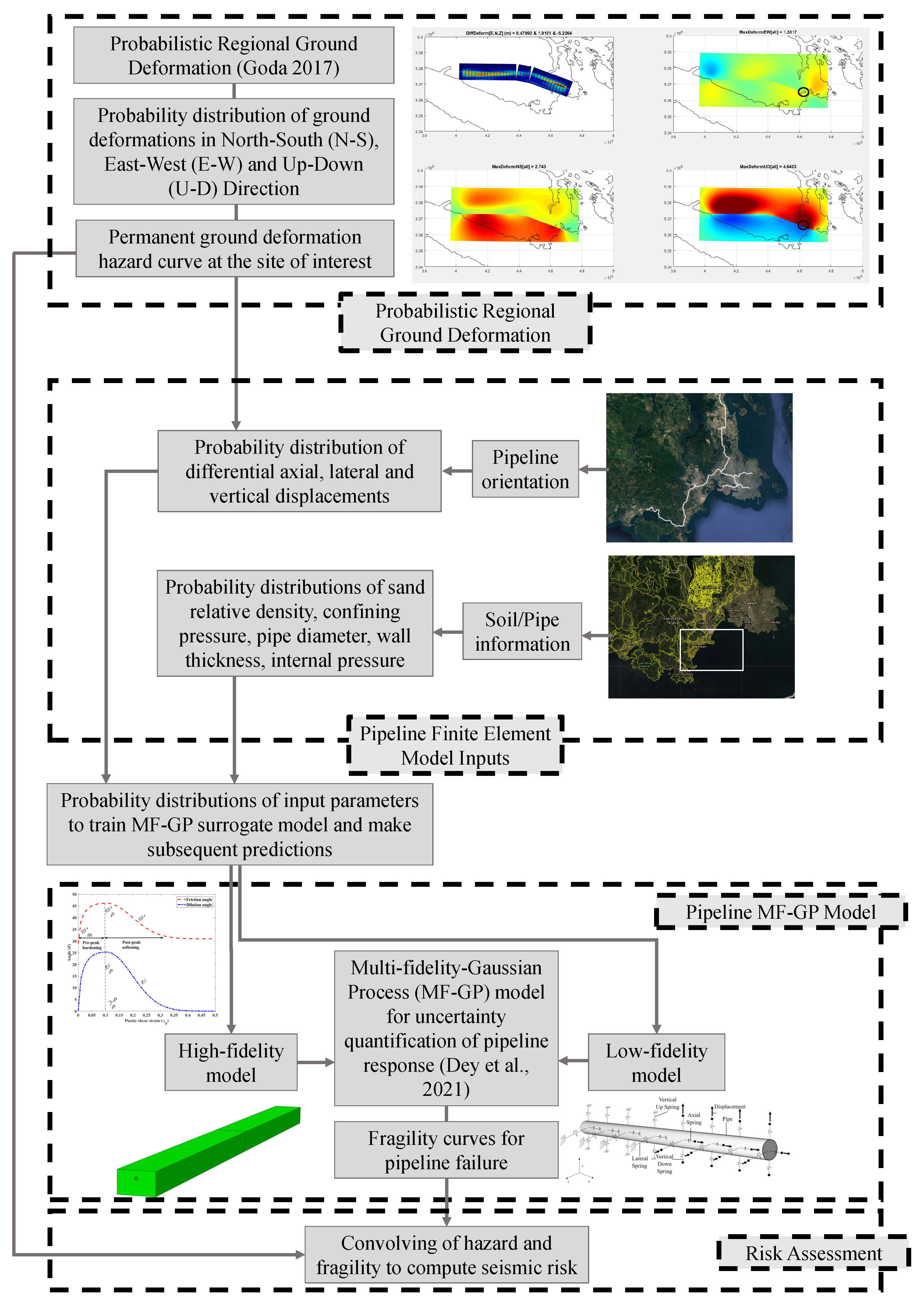
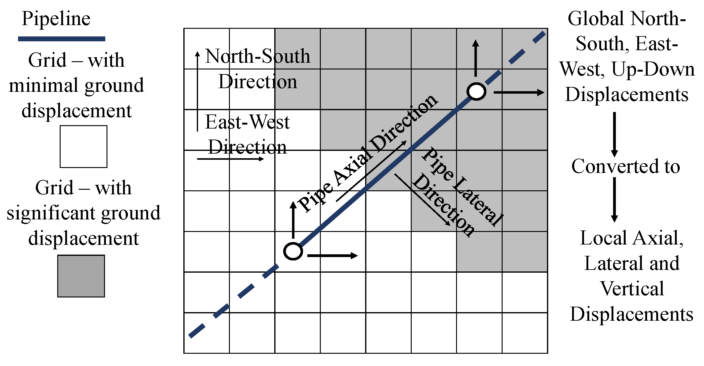
2. Integrated Risk Assessment Method for Buried Pipelines Due to Fault-Rupture-Induced Permanent Ground Deformations

The proposed methodology first characterizes the permanent ground deformation over a region probabilistically, using the approach by [12]. Thereafter, the pipeline structural response is evaluated using finite element analysis and the MF-GP surrogate model, as discussed in [32]. Finally, pipeline fragility and seismic hazards are convolved to determine seismic risk to the pipeline. To consider uncertainties in the pipe structural response, variations in the pipe’s geometric properties, the pipe’s material properties, soil conditions, the pipe’s operating conditions and variations in permanent ground deformation loading are considered in this assessment. Figure 1 presents the proposed method as a flow chart.
At first, the probabilistic regional ground deformation approach computes ground deformations over a region using statistical models for earthquake source parameters, simulated earthquake slip models and analytical Okada equations. To do so, fault geometry is first defined based on regional geological and seismological studies. It is then discretized into sub-faults to allow heterogeneous slip distribution over the fault plane. An earthquake scenario is then defined based on regional seismicity and is typically represented by truncated exponential and characteristic earthquake recurrence model. A logic tree approach is used to consider uncertainties in various parameters involved in the earthquake occurrence modeling. Thereafter, based on an earthquake scenario, earthquake source parameters are sampled from statistical scaling relationships derived from the earthquake rupture model database. Thereafter, realistic fault slip fields are generated and ground deformations are finally computed using Okada equations, all constrained to the fault geometry set initially. The resultant probabilistic ground deformations are strictly of tectonic origin and can be obtained at any location within a region. More importantly, differential probabilistic ground deformation between any two points can also be estimated.
Subsequently, the pipeline’s structural response is assessed using finite element analysis and the MF-GP surrogate model. The pipeline’s structural behavior is a combined function of the pipe’s geometric properties, pipe’s material properties, soil’s material properties, pipe’s operating conditions and permanent ground deformation loading conditions. Hence, uncertainties in these parameters will propagate to uncertainties in the pipeline structural response. To account for the uncertainty in the pipeline response, pipeline structural response data corresponding to numerous scenarios were generated using finite element analysis. These numerous scenarios consider uncertainties in the influencing parameters, such as uncertainty in pipe geometric and material properties, uncertainty in soil conditions, uncertainty in pipe operating conditions and uncertainty in permanent ground deformation loading. Since 3-dimensional complex experimentally evaluated numerical models were used for finite element analyses, performing large numbers of analyses was not feasible due to the limitation in computational resources. Hence, the MF-GP surrogate model was first trained using data from small numbers of high-fidelity (HF) finite element models and large numbers of low-fidelity (LF) finite element models. This trained MF-GP surrogate model was thereafter used to predict structural response data for variations in all the influential parameters.
Data used for training and predicting pipeline response were peak axial compressive strain and peak axial tensile strain. The uncertainty in permanent ground deformation loading was obtained from the generated probabilistic ground deformations. By analyzing the finite element models to generate training data for the MF-GP surrogate model, pipeline orientation maps and differential permanent ground deformation between two sides of the rupturing surface resulted in varying displacement boundary conditions and pipeline-fault plane angles.
Finally, from the trained MF-GP surrogate model, probability density functions of peak axial compressive and tensile strains were obtained to understand the statistics of the generated strains. Additionally, to compute seismic risk, fragility curves were generated from the trained MF-GP surrogate model based on failure strain limits of some pipeline design guidelines and convolved with the probabilistic ground deformation hazard curve.

3. Probabilistic Ground Deformation Hazard Assessment for Victoria, British Columbia

The LRVFZ is located in the vicinity of the City of Victoria and is worthy of consideration for seismic risk assessments in the region, as discussed in [22,23,24]. To generate ground deformations probabilistically due to fault ruptures, the method proposed in [12] was adopted.

3.1. Leech River Valley Fault Zone (Lrvfz) Source Characterization and Rupture Occurrence

The LRVFZ consists of a north–northeast dipping zone, as reported in [23]. The north–east ward reverse faulting dipping region of the LRVFZ is about 70 steep and extends for about 60 km, as reported in [22,25,26]. The fault geometry of the LRVFZ in the current study was adopted from [25]. A fault length of 67.8 km was assumed, accordingly. A dipping angle of 70 was used in accordance with [25], resulting in a fault width of 25 km. The fault geometry was thereafter divided into a total of 525 sub-faults: 35 along the strike and 15 along the dip. Fault ruptures in the LRVFZ fault plane were simulated by rectangular finite-fault sources. The earthquake magnitudes were modeled based on [33,34]. A truncated exponential model and a characteristic model were used to define the magnitude versus annual frequency relationship. Details of the earthquake modeling approach for the LRVFZ can be found in [27]. First, the slip rate was obtained by considering a representative slip rate of 0.25 mm/year, as found in [25,35,36]. The fault zone area was calculated based on the adopted fault length and width. A shear modulus of 35 GPa was adopted in the calculations based on [27]. A value of 0.796 was used for the slope parameter of the truncated exponential model based on [37].
A minimum earthquake magnitude of 6 was used according to [25]. The magnitude intervals to define probability density value for the characteristic part and the magnitude intervals for the characteristic part were set to 1.0 and 0.5, respectively, based on [25,33]. For each of the two earthquake magnitude models, variations in discrete values of these parameters were considered. These parameters were randomly selected using a logic-tree approach in association with a combination of characteristic and truncated exponential magnitude–annual frequency relationships to characterize fault ruptures and their occurrence. Once a fault rupture occurs within a specified magnitude range of 0.1 bin in between 6.0 and 7.7, earthquake magnitude is generated from a discrete distribution. Subsequently, stochastic source models are generated according to [12] for that given earthquake magnitude using earthquake source scaling relationships. These relationships can be found in [19], which consider uncertainties in fault rupture by means of variations in both geometrical parameters and slip distributions. One-thousand stochastic sources were generated for the selected magnitude range of 0.1, and one of them was randomly selected for extraction of fault plane and fault slip information.

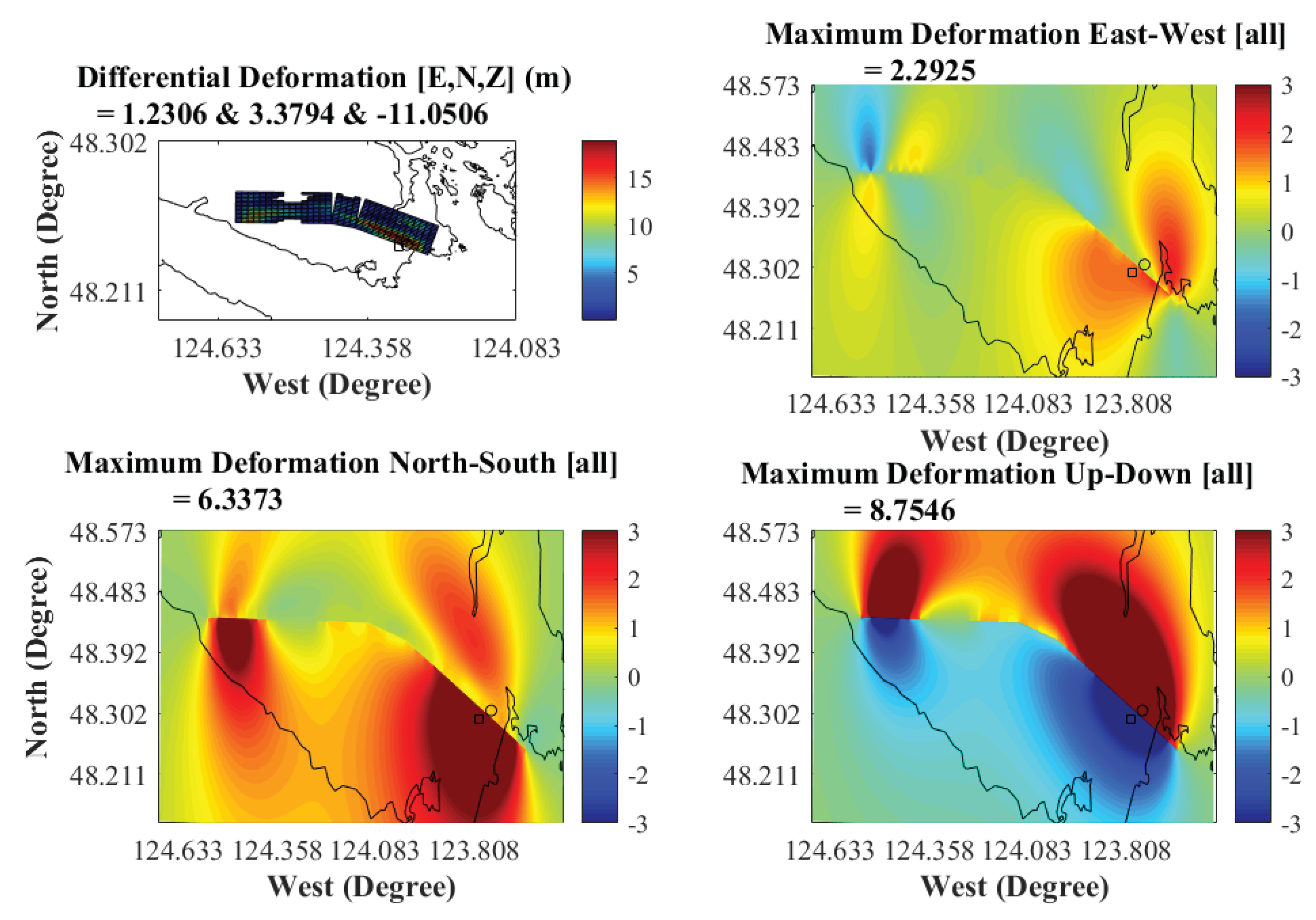
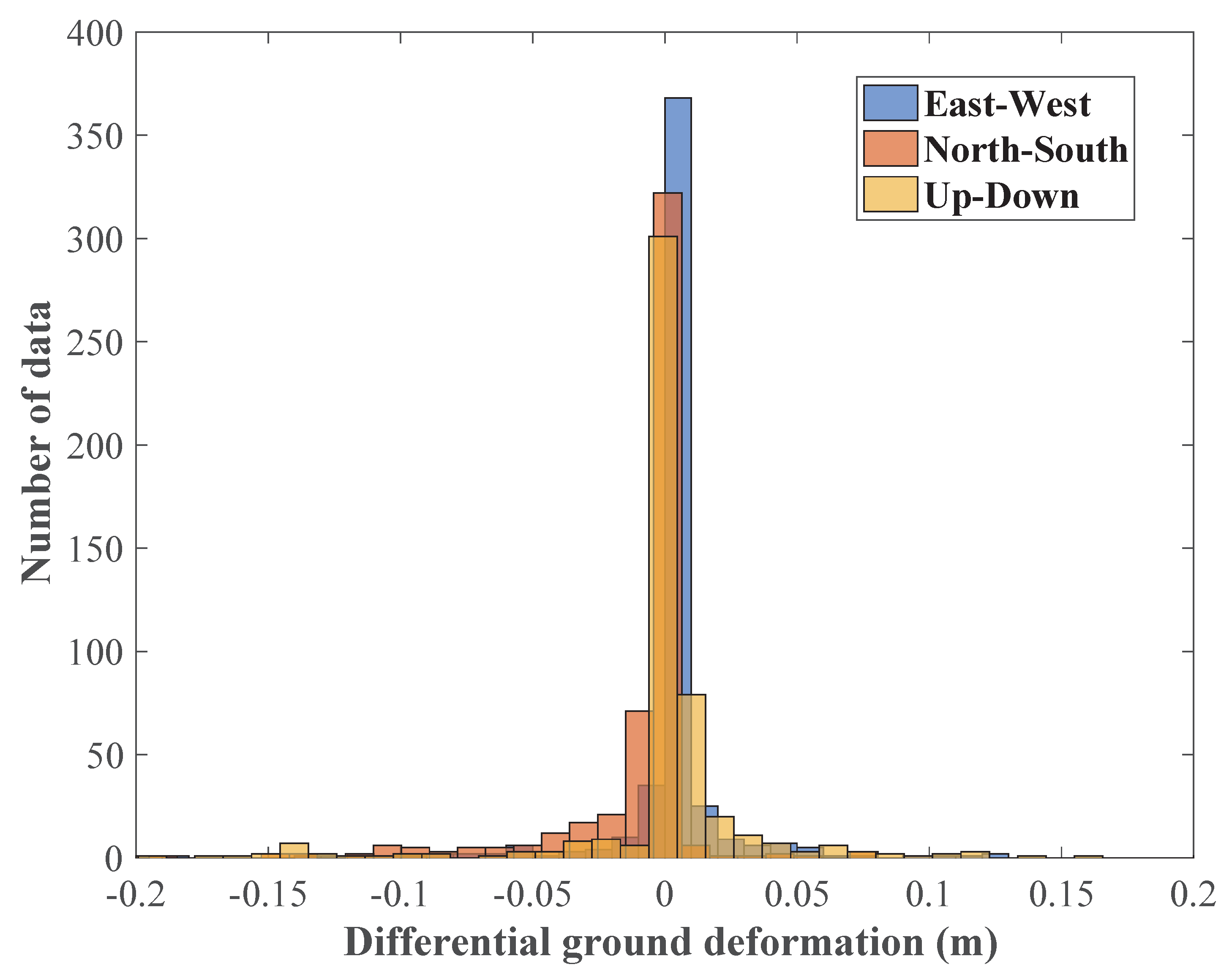
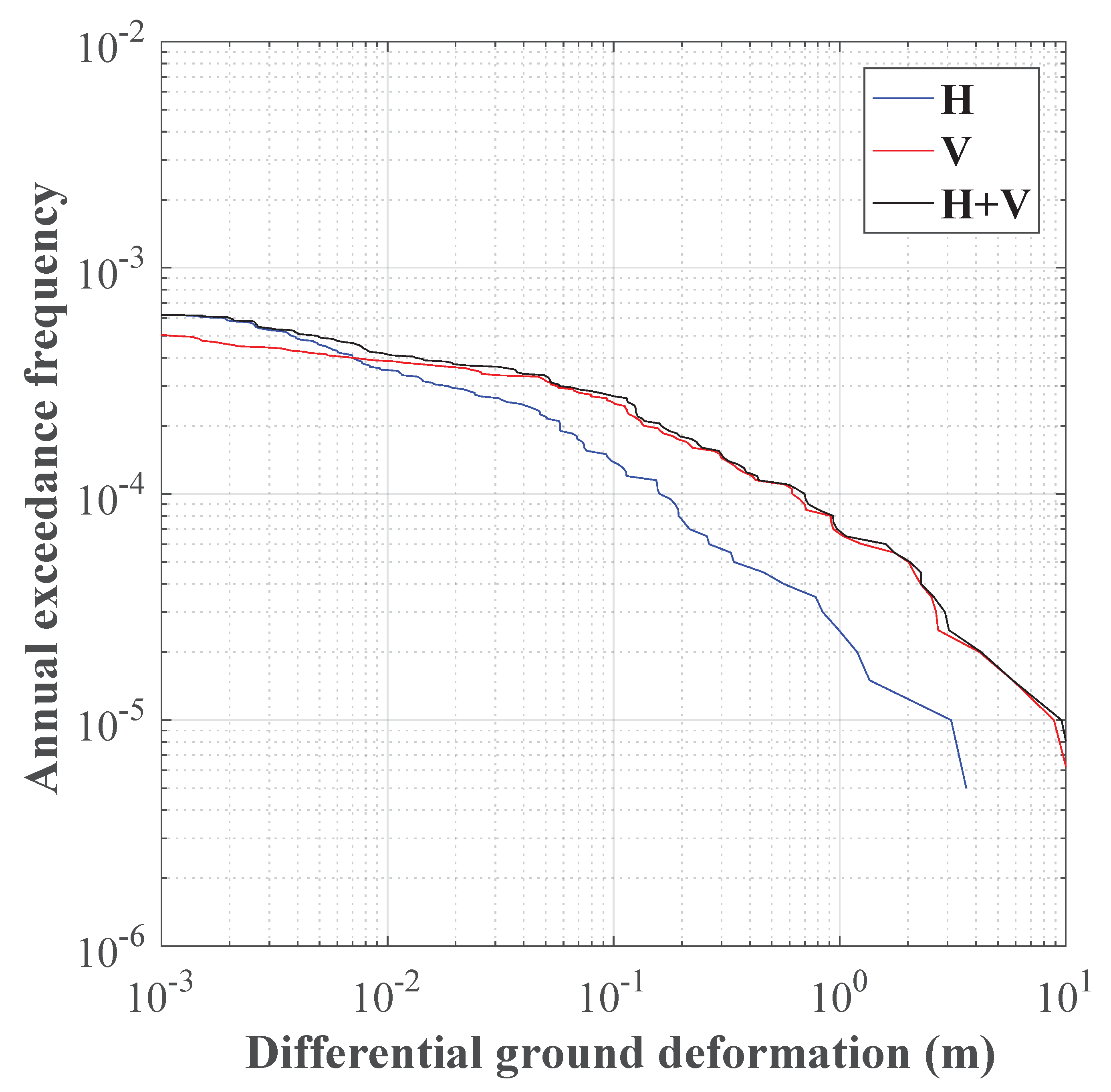
3.2. Probabilistic Ground Deformation Hazard Assessment

The probabilistic ground deformation hazard was computed based on [38]. In the ground deformation computation phase, the randomly selected source parameters were utilized to define the fault plane. Additionally, an earthquake slip field was generated randomly based on the spatial slip distribution parameters, which were also generated from the scaling relationships by [19]. An iterative approach was adopted to ensure consistency between the generated fault length, width and mean slip by matching the target and simulated seismic moment. Subsequently, Okada equations were used to compute surface displacements of an elastic half space due to a rupture in a rectangular fault. The inputs for the Okada computations were rake angle and slip value, in addition to the rupture geometry. The rupture geometry parameters included the strike angle, dip angle, fault length, width and depth. Depth indicates the depth of the fault centroid. Strike is the azimuth angle of fault trace with respect to north. Dip angle is the angle between the fault plane and horizontal plane. Fault length is the dimension of the fault along the strike. Fault width is the dimension of the fault along the dip. Rake angle is the angle between the hanging wall movement direction and that of the strike. Slip defines the value of hanging wall movement. To limit computational time, Okada equations were pre-computed at locations of interest in the east–west, north–south and up–down directions for every sub-fault by considering a unit displacement (reverse faulting). Post stochastic synthesis of slip for all sub-faults, precomputed deformation values for unit slip could be scaled to derive the final ground deformations using Okada equations based on [20]. Since the ground deformation computed using Okada equations are physically consistent for a given rupture, differential deformations in the east–west, north–south and up–down directions could also be evaluated for the two sites of interest and used for finite element analyses. A thorough review of the gas pipeline network of the City of Victoria was performed, and a pipe susceptible to differential permanent ground deformation—( 48 25 59.49 N, 123 31 42.80 W) to ( 48 26 27.67 N, 123 29 6.64 W)—was identified.

4. Finite Element Models of Buried Pipelines

The finite element models used in the current analyses were both HF models and LF models. The finite element models were created in finite element analysis software ABAQUS [39]. References [2,40,41,42,43,44,45,46,47,48,49,50] previously employed shell element pipes with surrounding continuum soil to analyze pipeline response undergoing fault rupture deformations. The computationally expensive HF model in the current study was based on this approach and follows the model in [31]. Both the HF and LF models were created in accordance with [32].
Since uncertainty quantification exercises require large numbers of cases to be analyzed, it is practically not feasible to run HF models for all the cases. Hence, a multi-fidelity uncertainty quantification approach was adopted where a small number (tens) of HF models and a large number (hundreds) of LF models were used to train a MF-GP surrogate model. The primary difference between the finite element models in [32] and the current study is that the former assumed no variations in the differential ground deformations between two sides of the fault rupture. Hence, the end displacement boundary conditions were fixed values for all the cases. The current study considered uncertainty in the differential ground deformation between two sides of the fault rupture. This uncertainty in the differential ground deformation translates to variable pipe-fault crossing angle and variable end boundary conditions in the pipe and soil faces.

4.1. Variation in Model Parameters

To conduct an uncertainty quantification exercise, variations in pipeline geometrical parameters, such as pipe diameter and wall thickness, were considered. The pipeline diameter at the location of study is 114 mm (email communication with Fortis BC). Variations in pipe diameter from 104 to 124 mm were considered. Pipe wall thickness was varied from 6.02 to 17.1 mm, which is the available range of wall thickness for the given pipe diameter. Additionally, among operating conditions, internal pressure was varied from no pressure up to a maximum of 550 kPa (email communication with Fortis BC). The soil at the site is sandy in nature (BC Soil Information Finder Tool). Uncertainty in the sandy soil conditions was considered by varying confining pressure and relative density. Mean confining pressure of 39 kPa was assumed with values ranging from 7.8 to 70 kPa, and mean relative density of 80 percent was assumed; values ranged from 55 to 95 percent. The effect of uncertainty in permanent ground deformation due to fault rupture was considered by varying the axial, lateral and vertical displacement boundary conditions in the finite element analyses. In this analysis, differential east–west, north–south and up–down displacements were varied from −0.185 to 0.216, −0.458 to 0.079 and −1.238 to 0.219 m, respectively, which is consistent with the values obtained from the probabilistic ground deformation at the site of interest.

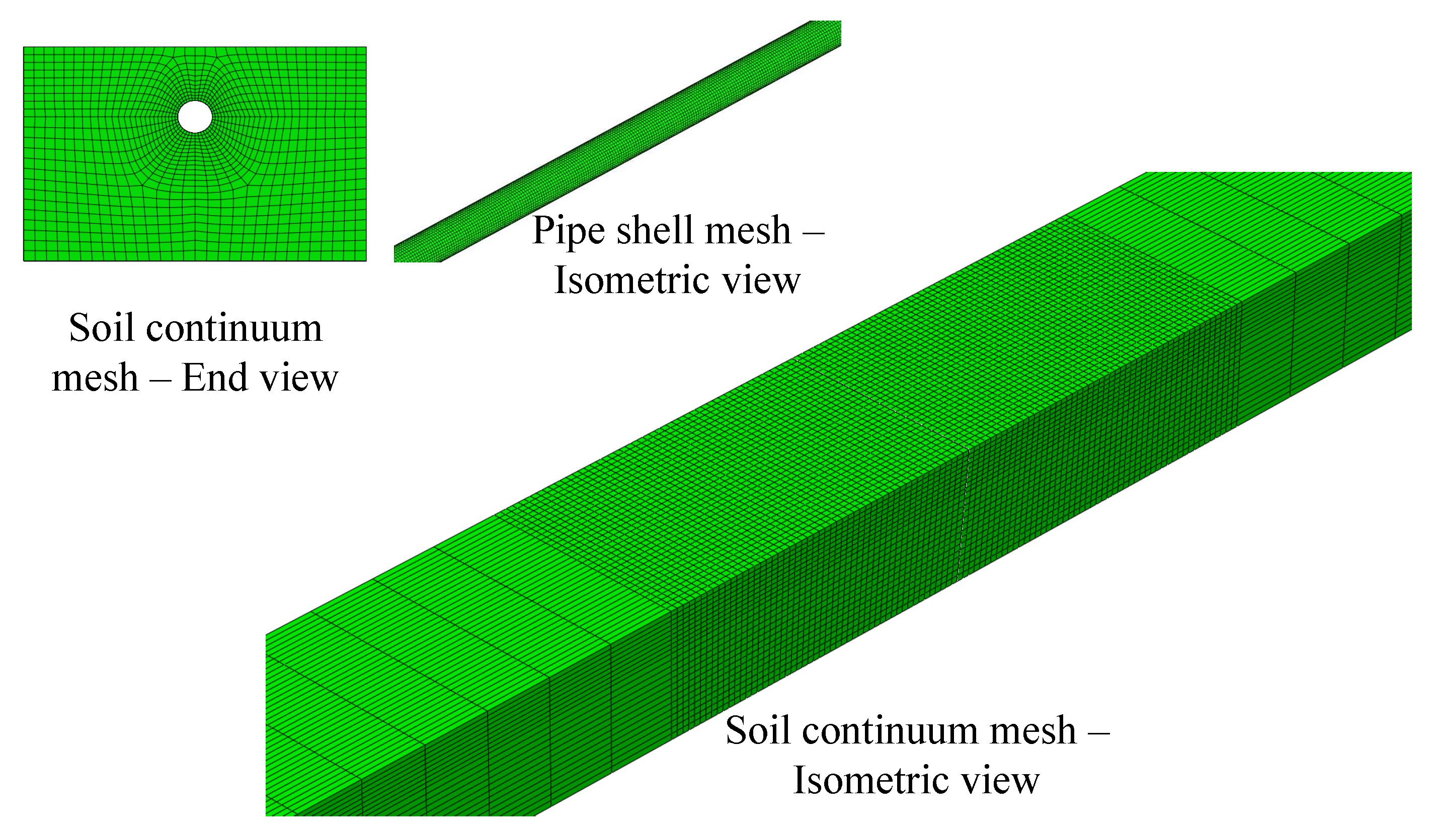
4.2. High-Fidelity Fe Model

A total of 30 HF models were created. The pipeline segment was modeled by employing 4-noded general reduced integration shell elements (S4R element). The soil continuum was modeled using three-dimensional reduced integration stress elements (C3D8R element). A mesh convergence study was performed, and an optimal mesh size was chosen accordingly. Pipe mesh size of 25 mm and soil mesh size surrounding the pipe of 10 mm were used. Figure 2 shows how the displacement boundary conditions for the finite element analyses were obtained from the regional ground deformations. As shown in the figure, differential ground deformations between the two ends of the pipe segment in the north–south, east–west and up–down directions were converted in the pipe local axial, lateral and vertical directions. A sample HF-FE model mesh is shown in Figure 3. The figure presents a soil continuum mesh and the shell pipe mesh. The pipe material is polyethelene PE80, and accordingly, a Young’s modulus of 800 MPa, Poison’s ratio of 0.4, yield strength of 21 MPa and ultimate strength of 30 MPa were considered. Sand shear strength response is a function of the confining pressure and relative density and is directly dependent on the internal angle of friction [51,52,53,54,55]. The salient features of a sand constitutive relation used are its elastic stiffness, pre-peak hardening behavior, peak strength and post-peak softening behavior [56,57]. Appendix A presents the soil constitutive equations used in the high-fidelity finite element model.
On average, each HF finite element model took 48 h to run, utilizing a 3.20 GHz eight-core processor with 32 GB of RAM. This model was found to predict local buckling in the majority of cases when the pipe was under compressive forces. Additionally, a few cases of tensile rupture were also noted when the pipeline came under tensile forces. The study in [32] considered variations in the pipe-fault crossing angle but utilized peak axial strain observations from discrete fault displacements, such as at fault displacements of 100, 200, 300 mm from all the HF and LF analyses to train the MF-GP surrogate model. In the current study, however, peak axial strains were obtained at the end of each analysis. Each analysis was designed to have pipe end differential ground deformation uniformly randomly selected from the ranges obtained previously.

4.3. Low-Fidelity Fe Model

The pipe was modeled using 3-noded quadratic PIPE32 elements, constituting a Timoshenko beam formulation, allowing both shear and bending deformation. The soil springs supporting the pipe in the mutually perpendicular axial, lateral and vertical directions were modeled using 3D pipe–soil interaction elements PSI34. These elements allow for bi-linear, elastic, perfectly plastic force displacement responses when simulating the soil resistance to the pipeline. Appendix B presents the relations used for computing the soil springs for the low-fidelity pipe-soil model. One end of the spring was connected to the pipe node and the other end is connected to the ground. The ground ends were assigned to be fixed on the stationary side of the fault. The ground ends were assigned a certain movement displacement boundary condition on the moving side of the fault. The LF finite element model represented a 100 m-long pipe segment and was made up of a total of 400 elements. Based on a mesh-sensitivity study, the element length was chosen to be 0.5 m. Out of the 400 elements, 200 elements were PIPE32 elements and 200 elements were PSI34 elements. The soil resistances were calculated based on [58]. On average, each LF finite element model took 15 min to run utilizing a 3.20 GHz eight-core processor with 32 GB of RAM. Figure 4 shows a sample comparison between high-fidelity and low-fidelity models for peak compressive strains generated against fault displacement magnitudes. The high-fidelity model is able to capture local buckling, and hence captures significantly higher strains in comparison to the low-fidelity model.

5. Uncertainty Quantification Using Multi-Fidelity Surrogate Modeling

It is evident from works by [59,60,61,62,63,64,65,66,67,68] that variations in soil conditions can impact pipeline structural response significantly. Additionally, pipe geometry, including diameter and wall thickness, can also influence the pipeline’s structural response, as established by [63,65,66]. Uncertainty quantification studies typically require a large number of scenarios to be analyzed to achieve sufficient accuracy in prediction. Some of the more commonly used uncertainty quantification techniques include simulation-based techniques, such as Monte Carlo simulations [69,70], and surrogate model-based techniques, such as polynomial chaos expansion [71,72], neural networks [63,73], radial basis functions [74] and the kriging method [75,76]. Monte Carlo simulations require a large number of scenarios to be run to achieve desirable accuracy. Similarly to that, the surrogate model-based methods also involve training a surrogate model using data from several analyses, and thereafter, using it to predict data for a large number of cases using a Monte Carlo simulation. Both approaches practically require a large number of analyses to be performed. Hence, its quite reasonable that traditionally, uncertainty quantification exercises for buried pipelines have been performed using simplified numerical models or analytical models [1,7,59,60,61,62,63,64,65,66,67,68] requiring minimal computational effort.
An uncertainty quantification exercise allowing for maintaining the intricacy and reliability associated with detailed pipe–soil numerical models will provide deeper and realistic insights into the behavior of the pipeline. Solving detailed pipe–soil numerical analysis problems, such as the current one at hand, involving continuum elements with non-linear soil constitutive relations and geometric nonlinearity and contact nonlinearity, requires a significant amount of computational effort. Hence, a multi-fidelity surrogate—multi-fidelity Gaussian processes (MF-GP) [77,78] was used to quantify uncertainty in the buried pipeline responses in Victoria, British Columbia due to fault-rupture-induced ground deformations. Appendix C presents some of the relations for a MF-GP. Reference [32] successfully applied the technique to study this problem in a hypothetical reverse faulting case. MF-GP learns from a small number of HF data (in the order of 10 s) and a large number of LF data (in the order of 100 s) and predicts data as well as HF. This approach helps in reducing enormous amounts of computational effort, as it allows for learning from a large number of computationally inexpensive LF data instead of an equal number of computationally expensive HF data.
Strain-based analysis approaches are suitable for displacement-controlled loading conditions, as detailed in [79]. The analysis for a pipeline undergoing deformations as a result of differential ground deformation loading is a displacement controlled analysis. Hence, the strain-based analysis approach was adopted here to compute pipeline failure. The pipeline failure strain is computed using deterministic approaches. The axial compressive strain limit based on [58] for ground movement caused hazard to pipelines was adopted as follows:
p c = 0.5 ( t / D ) 0.0025 + 3000 ( p D / 2 E t ) 2
where p c is compressive strain limit, t is the pipe wall thickness, D is the pipe diameter, p is the internal pressure and E is the Young’s modulus. The axial tensile strain limit based on [58] is given as 2 percent for ground-movement-related hazards to pipelines. References [1,7] have considered failure due to axial tensile and compressive strains to study the performances of buried pipelines due to fault-rupture-induced permanent ground deformation. Reference [7] utilized the strain limit from [58] to define failure state. Reference [1], on the other hand, used failure states corresponding to 10 percent and 90 percent failure probabilities based on [80].
The MF-GP surrogate model created was used to predict failure probabilities at varying levels of permanent ground deformation to compute the fragility curves. Previously, references [1,7] successfully utilized the fault displacement as an intensity measure to assess the seismic performance of buried pipelines due to fault ruptures. For the current study, permanent ground deformation at each point in the region of interest is available probabilistically. Additionally, the load acting on the pipe segment was a function of the differential ground deformation between the two ends of the pipe segment. Hence, differential ground deformation was chosen as an intensity measure to derive the fragility curves. The ground deformation hazard curve was convolved with the fragility relations to come up with the seismic risk. This method is inspired by the approaches to combine ground motion hazard curves with fragility functions to compute the yearly rate of structural failure [81,82,83,84]. Fragility curves in general are created using a variety of techniques, such as with the help of observed data, static analyses and dynamic structural analysis [85]. The vulnerability of a structure can be expressed as a cumulative probability of it reaching a failure limit state as a function of the load intensity it is subjected to. Generally, a fragility function is used for this purpose and assumes the shape of a log-normal function. The cumulative lognormal function was adopted in accordance with [85], as shown below in (2):
P d i | I M = x = υ ln ( x θ ) λ
wherein the probability that a structure will be at a failure state ( d i ) caused by a load intensity I M = x is P d i | I M = x ; υ denotes the standard normal cumulative distribution function; θ is the load intensity level denoting a failure probability of 50 percent or the median of the fragility function; λ signifies the standard deviation for l n ( I M ) . Initially, realistic values for the parameters defining the fragility equation are assumed. The parameters are finally obtained by maximizing the logarithm of the likelihood function as shown below (3):
θ ^ , λ ^ = a r g m a x j = 1 m ln n j z j + z j ln ϕ ln ( x j θ ) λ + n j z j ln 1 ϕ ln ( x j θ ) λ
where m is the number of load intensity levels. At each load intensity level I M = x j , it is assumed that the structural analyses produce z j failures out of n j analyses. To derive the fragility curves, the MF-GP surrogate model is trained with peak axial strain data obtained at the end of all the finite element analyses. The number of failures at incremental fault displacements is calculated using [58] compressive strain limit criterion. The load intensity (fault displacement) vs. probability of failure data points are thereafter used for generation of the fragility curves.
The annual probability of failure P f is computed by convolving the developed fragility curves and the derived hazard curve at this particular site. The intensity measure considered for this problem is differential ground deformation. The annual rate of failure was computed according to [85] as:
P f = x P d i | I M = x d H ( x ) = x υ ln ( x θ ) λ d H ( x )
where H ( x ) is a hazard curve for the intensity measure differential ground deformation. The hazard curve provides the annual rate for exceedance of differential ground deformation. d H ( x ) is the absolute value of the derivative of the hazard curve.

6. Results and Discussion

This section presents results regarding probabilistic ground deformation in the City of Victoria and their further application to quantify uncertainty in the structural responses of buried pipelines. The results also include cross-validation of the MF-GP surrogate model. The pipeline response parameters of interest, namely, peak axial compressive strains and peak axial tensile strains, were considered. Uncertainty in pipeline response was studied by generating probability density functions of pipeline peak axial compressive and tensile strains. A sensitivity analysis was also included to identify the most influential parameters on the pipeline’s response.

6.1. Probabilistic Ground Deformation Hazard Estimation for Lrfz

Figure 5 presents a sample critical rupture scenario including the slip distribution along the fault and computed ground deformations in the north–south, east–west and up–down directions. The location of interest in this study, as identified with a circle and square, is shown to have significant differential ground deformations in Figure 5. Significant differential ground deformation can be observed along the boundary of the fault geometry. Since ground deformations computed using Okada equations regionally are physical consistent, the ground deformations computed for each scenario at point 1 and point 2 have physical dependency. Thus, once the probabilistic ground deformations were computed at point 1 ( 48 25 59.49 N, 123 31 42.80 W) and point 2 ( 48 26 27.67 N, 123 29 6.64 W), the differential probabilistic ground deformations were obtained by computing the differences in ground deformation between point 1 and point 2 in the corresponding north–south, east–west and up–down directions. Figure 6 shows the histograms of differential probabilistic ground deformation between point 1 and point 2. The peak of differential ground deformation in the histogram was found to have significant non-zero values. Figure 7 shows the relation obtained for annual exceedance frequency with that of the differential permanent ground deformation between site 1 and site 2. These hazard curves show a decrease in annual exceedance rate with the increases in ground deformation values. These hazard curves provide us with quantitative information regarding the degree of hazard at the site of interest. These curves were later used to compute seismic risk. Differential ground deformation of 1 m at the site of interest was found to have an annual exceedance frequency of 10 4 .

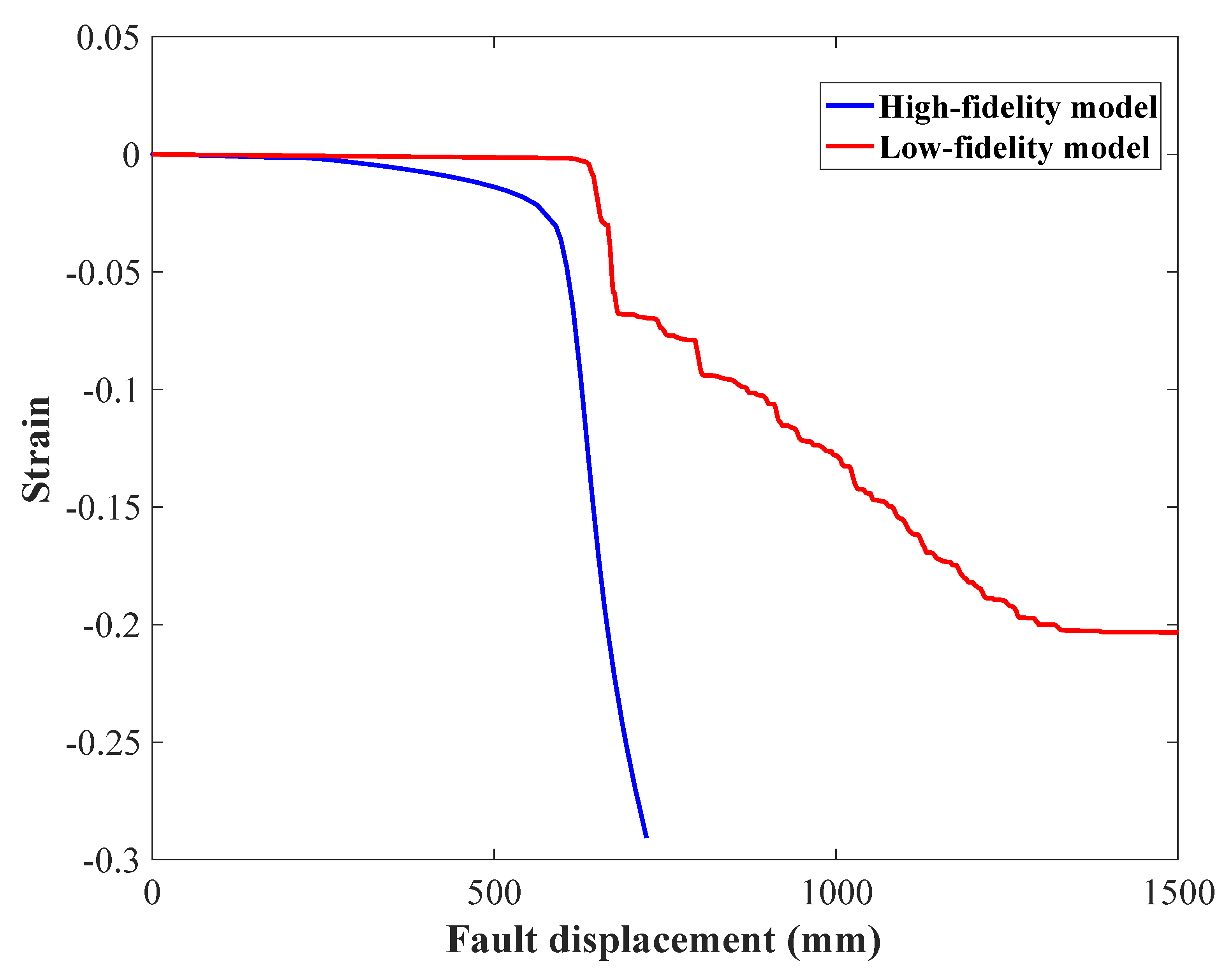
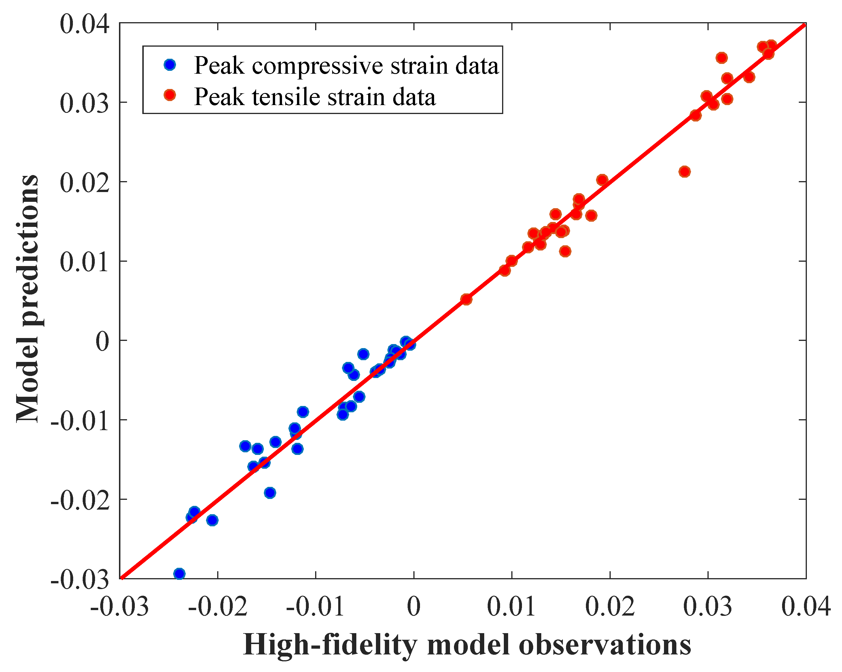
6.2. Cross-Validation and Uncertainty Quantification of Pipeline Response

The peak axial compressive strains and peak axial tensile strains from the HF and LF-FE models were utilized to train the MF-GP surrogate model. Peak tensile and compressive axial strains were obtained at the last instants in the 30 HF and 500 LF-FE analyses. This was so done to ensure that the intended displacement boundary condition would be fully applied at the instant of strain extraction. To ensure the validity of the developed MF-GP surrogate model, a k-fold cross-validation technique was adopted. To do so, HF data were divided equally into six parts. At first, the first part was used to test the surrogate model, and the rest of the data were used to train the surrogate model. Similarly, next, the second part was used to test the surrogate model, and the rest of the data were used to train the surrogate model. This process was repeated for all the parts. The validity of the MF-GP surrogate model was measured with the coefficient of determination (R-squared). Figure 8 presents the cross-validation results for both the axial tensile strains and axial compressive strains. High values of the coefficient of determination of 0.92 and 0.96 were obtained for the axial compressive strains and axial tensile strains, respectively. Figure 8 shows that the predicted values for axial tensile strain and axial compressive strain are more or less aligned along the line for the coefficient of determination being equal to 1. Axial tensile strain values can be observed to range from 0 to 0.04, whereas axial compressive strain values were found to range from 0 to −0.03. Reference [7] reported a maximum tensile strain of 3.39 percent and maximum compressive strain of 0.13 percent in the pipeline-fault rupture problem. Hence, the results obtained from the current study can be considered reasonable. Compressive buckling was identified as the primary failure mode in this problem. For peak axial tensile strains, the most sensitive parameters were identified to be pipe’s outer diameter, sand confining pressure and differential ground deformation in the vertical direction. Figure 9 shows the sensitivities of the input variables and those of the generated compressive strains. For peak compressive strains, sand relative density was found to be the most sensitive input parameter, at about 35 percent. Secondly, axial displacement, lateral displacement and vertical displacements were found to have sensitivities in the range of 15 to 25 percent. Pipe outer diameter, wall thickness, sand confining pressure and internal pressure were found to have sensitivities of less than 5 percent. These observations are reasonable, as the boundary conditions of axial, lateral and vertical displacements are expected to influence the failure of a pipe directly. Additionally, the relative density of the sand is expected to influence the soil resistance, thereby influencing pipe failure.
Figure 10 presents the generated probability density functions for the pipeline’s peak axial tensile and compressive strains for the given location. The most probable peak compressive strain was found to be about 1 percent. The most probable peak tensile strain was found to be around 2 percent. The predicted axial tensile strains were observed to vary from 0 to 0.07. The predicted axial compressive strains were found to vary between 0 and −0.02. Both the density functions were found to have a flatter slope towards the 0 strain level. A cumulative lognormal function based on [85] was used to generate fragility curve for the pipeline at the site. To evaluate damage, strain limit based on [58] has been used. Figure 11 shows the probability of pipeline damage at the site of interest as a function of differential ground deformations. The fragility curves derived in Figure 11 rely on Equation (3). These fragility functions are specific to this site and the pipeline’s properties. From the fragility curves, it is evident that the pipeline here is more prone to failure due to compressive strains than tensile strains. The fragility curve based on failure due to compressive buckling was found to increase rapidly, and the slope gradually reduces to reach probability of failure 1 at about 1400 mm differential permanent ground deformation. The tensile fragility curve gradually reached a probability of failure of 0.55 at about 1400 mm of differential permanent ground deformation. It is to be noted here that, based on the ultimate strain capacity of PE 80 pipes, no significant failure can be observed. The seismic risk or the annual probability of failure due to compressive buckling was calculated by convolving the compressive fragility curve and the seismic hazard curve to be 1.5 percent in 50 years. Additionally, the seismic risk or the annual probability of failure due to tensile rupture was calculated by convolving the tensile fragility curve and the seismic hazard curve to be 0.6 percent in 50 years. Baker [85] reported probabilities of failure of 1.3, 1.2 and 1.1 percent in 50 years for the set of fragility curves and hazard curves considered. Hence, the risk computed in the current study is deemed reasonable.

7. Conclusions

In this paper, an integrated seismic risk assessment technique for buried pipelines due to fault-rupture-induced permanent ground deformation hazard was developed. It can be applied both regionally and at specific sites. To do so, a previously developed probabilistic ground deformation approach was employed. Additionally, a previously developed method to quantify uncertainty in a pipeline’s structural response using a MF-GP surrogate model was used. The primary contribution of this work was to bridge these two approaches suitably to present an integrated seismic risk assessment approach for buried pipelines. The method considers variability in regional fault source characteristics, site specific soil conditions, pipeline geometry and operating conditions to quantify uncertainty in the pipeline’s structural response. The method considers uncertainty in a comprehensive manner in various aspects and levels of the assessment, and utilizes experimentally evaluated rigorous geotechnical numerical models in an efficient manner. The method uses an MF-GP surrogate model to ensure efficiency.
The developed method was used to illustrate a case study for the city of Victoria’s buried gas pipeline. The MF-GP surrogate model was successfully cross-validated with an excellent coefficient of determination between HF observed values and MF predicted values. Finally, the uncertainties in generated peak axial tensile and compressive strains were presented as probability density functions. The seismic risks of pipeline failure due to compressive buckling and tensile rupture at the site considered were computed to be 1.5 percent and 0.6 percent, respectively, in 50 years. Although the case study performed here was for a specific pipe location, the same approach can be used for multiple locations of concern over a region. In that case, either separate MF-GP surrogate models can be created for each site or a global MF-GP surrogate model can be created. In the latter case, wide variations in the influential variables values would need to be considered. These variations would account for every possible combination for all the sites. Separate prediction data can be used to evaluate each site individually.
This study established that the seismic risk assessment of buried continuous pipelines on a regional scale can be performed using experimentally validated detailed finite element models. On the one hand, the method allows for maintaining the intricacies of the detailed pipe–soil numerical model, and on the other hand, the method allows for use of stochastic source modeling and Okada equations instead of regression equations to characterize regional ground motion probabilistically. Although the method proposed is illustrated for a case study in the city of Victoria, the developed method can be applied to evaluate seismic risk to buried pipelines due to permanent ground deformation in any seismically active region.

Author Contributions

Conceptualization, S.D and S.T.; methodology, S.D.; software, S.D.; validation, S.D.; formal analysis, S.D.; investigation, S.D.; resources, S.T.; data curation, S.D.; writing—original draft preparation, S.D.; writing—review and editing, S.D. and S.T.; visualization, S.D.; supervision, S.T.; project administration, S.T.; funding acquisition, S.T. All authors have read and agreed to the published version of the manuscript.

Funding

This research was funded by the Natural Science Engineering Research Council of Canada (NSERC) Discovery Grant (RGPIN-2019-05013).

Acknowledgments

The computer codes to generate regional probabilistic ground deformation in this paper was supplied by Katsuichiro Goda.

Conflicts of Interest

The funders had no role in the design of the study; in the collection, analyses, or interpretation of data; in the writing of the manuscript; or in the decision to publish the results.

Appendix A. High-Fidelity Constitutive Equations

The elastic modulus is derived as [86]:
E = K p a ( p / p a ) n
where p represents the sand confining pressure and p a represents the atmospheric pressure. K and n are constants: K = 150 and n = 0.5 [87,88].
The pre-peak mobilized friction angle ϕ and dilation angle ψ are obtained as [89]:
ϕ = ϕ i n + sin 1 2 γ p γ p p γ p + γ p p sin ( ϕ p ϕ i n )
ψ = sin 1 2 γ p γ p p γ p + γ p p sin ( ψ p )
The plastic shear strain at peak friction angle γ p p is obtained as [55]:
γ p p = γ c p p p a m
The strain softening parameter γ c p is:
γ c p = C 1 C 2 I D
where C 1 , C 2 and m are constants and need to be calibrated from experiments. Realistic estimates of C 1 = 0.22, C 2 = 0.11 and m = 0.25 were considered in this study. The friction angle at yielding ϕ i n was set to 29 .
The peak internal angle of friction ϕ p is obtained as [51]:
ϕ p = ϕ c + A ψ I R
The mobilized friction angle at critical state ϕ c was set to 31 , and the constant A ψ was set to 3 (tri-axial test conditions). The relative density index I R is obtained as [51]:
I R = I D ( Q ln p ) R
where, Q = 10 and R = 1 . ψ p is the peak dilation angle and can be calculated according to [51] as:
ψ p = ϕ p ϕ c k ψ
k = 0.5 for triaxial conditions [51]. The post-peak nonlinear strain softening zone is defined according to [56] as:
ϕ = ϕ c + ( ϕ p ϕ c ) exp γ p γ p p γ c p 2
ψ = ψ p exp γ p γ p p γ c p 2

Appendix B. Low-Fidelity Model Soil Springs

The soil resistances are calculated based on [58] as follows: The axial soil resistance T U is calculated as:
T U = π D ω c + π D H γ ¯ ( 1 + K 0 ) 2 tan δ
The lateral soil resistance P u is calculated as:
P u = M c h c D + M q h γ ¯ H D
The vertical up-resistance Q u is calculated as:
Q u = M c v c D + M q v γ ¯ H D
The vertical down-resistance Q d is calculated as:
Q d = M c c D + M q γ ¯ H D + M γ γ D 2 2
D denotes the pipe diameter, c denotes the soil cohesion representative of soil backfill, H is the depth to the pipe’s centerline, γ ¯ is the effective unit weight of the soil, γ is the total unit weight of soil, K 0 is the coefficient of pressure at rest, ω is the adhesion factor, δ is the pipe-to-soil surface interface friction angle ( = f ϕ ) , f is the coating factor and ϕ is the friction angle of the soil. M c h is the bearing capacity factor for clay in the horizontal direction, M q h is the bearing capacity factor for sand in the horizontal direction, M c v is the uplift factor for clay in the vertical direction and M q v is uplift factor for sand in the vertical direction. M c , M q and M γ are additional factors controlling the bearing capacity of the soil.

Appendix C. Multi-Fidelity Gaussian Processes

The MF-GP auto-regressive model by [78] can be represented as:
Z e x = ρ Z c x + Z d x ,
Z e represents the MF-GP and the HF-GP, and Z c represents the LF-GP. This way, the HF-GP is expressed as a sum of the difference GP and a scaling factor times LF-GP. Reference [90] provides the derivation of the MF-GP. The input data can be represented as:
X = X c X e = ( x 1 c , , x n c c , x 1 e , x n e e ) T
Z e ^ ( x ) = p ( x ) T n ^ + d ( x ) T D 1 ( J P n ^ )
where J = [ J c T , J e T ] T ; p ( x ) = [ ρ g ( x ) T , g ( x ) T ] T ; n ^ = ( P T D 1 P ) P T D 1 J ; and d ( x ) is expressed as:
d ( x ) = ρ σ c 2 r c ( x , x c ) ρ σ c 2 r c ( x , x e ) + σ d 2 r d ( x , x e )
P = g ( x 1 c ) T 0 g ( x n c c ) T 0 ρ g ( x 1 e ) T g ( x 1 e ) T ρ g ( x n e e ) T g ( x n e e ) T
D = σ c 2 R c ( X c , X c ) ρ σ c 2 R c ( X c , X e ) ρ σ c 2 R c ( X e , X c ) ρ 2 σ c 2 R c ( X c , X e ) + σ d 2 R d ( X e , X e )
Z e ^ ( x ) = n ^ + d ( x ) T D 1 ( J 1 n ^ )
where n ^ = ( 1 T D 1 1 ) 1 1 T D 1 J and P is a vector of ones. The predictor variance is obtained as
σ e ^ 2 ( x ) = ρ ^ 2 σ e ^ 2 + σ d ^ 2 d ( x ) T D 1 d ( x )

References

  1. Cheng, Y.; Akkar, S. Probabilistic permanent fault displacement hazard via Monte Carlo simulation and its consideration for the probabilistic risk assessment of buried continuous steel pipelines. Earthq. Eng. Struct. Dyn. 2017, 46, 605–620. [Google Scholar] [CrossRef]
  2. Robert, D.J.; Soga, K.; O’Rourke, T.D. Pipelines subjected to fault movement in dry and unsaturated soils. Int. J. Geomech. 2016, 16, 1–16. [Google Scholar] [CrossRef]
  3. Eidinger, J.M.; O’Rourke, M.; Bachhuber, J. Performance of a pipeline at a fault crossing. In Proceedings of the 7th US National Conference of Earthquake Engineering, Earthquake Engineering Research Institute (EERI), Boston, MA, USA, 21–25 July 2002. [Google Scholar]
  4. De Risi, R.; De Luca, F.; Kwon, O.S.; Sextos, A. Scenario-based seismic risk assessment for buried transmission gas pipelines at regional scale. J. Pipeline Syst. Eng. Pract. 2018, 9, 04018018. [Google Scholar] [CrossRef]
  5. Lanzano, G.; de Magistris, F.S.; Fabbrocino, G.; Salzano, E. Seismic damage to pipelines in the framework of Na-Tech risk assessment. J. Loss Prev. Process Ind. 2015, 33, 159–172. [Google Scholar] [CrossRef]
  6. Hwang, H.; Chiu, Y.H.; Chen, W.Y.; Shih, B.J. Analysis of damage to steel gas pipelines caused by ground shaking effects during the Chi-Chi, Taiwan, earthquake. Earthq. Spectra 2004, 20, 1095–1110. [Google Scholar] [CrossRef]
  7. Melissianos, V.E.; Eeri, M. Performance Assessment of Buried Pipelines at Fault Crossings. Earthq. Spectra 2017, 33, 201–218. [Google Scholar] [CrossRef]
  8. Stepp, J.C.; Wong, I.; Whitney, J.W.; Quittmeyer, R.; Abrahamson, N.; Toro, G.; Young, S.; Coppersmith, K.; Savy, J.; Sullivan, T. Probabilistic seismic hazard analyses for ground motions and fault displacement at Yucca Mountain, Nevada. Earthq. Spectra 2001, 17, 113–151. [Google Scholar]
  9. Youngs, R.R.; Arabasz, W.J.; Anderson, R.E.; Ramelli, A.R.; Ake, J.P.; Slemmons, D.B.; McCalpin, J.P.; Doser, D.I.; Fridrich, C.J.; Swan, F.H., III; et al. A methodology for probabilistic fault displacement hazard analysis (PFDHA). Earthq. Spectra 2003, 19, 191–219. [Google Scholar] [CrossRef]
  10. Budnitz, R.; Apostolakis, G.; Boore, D.M. Recommendations for pRobabilistic Seismic Hazard Analysis: Guidance on Uncertainty and Use of Experts; Technical Report; US Nuclear Regulatory Commission (NRC): Washington, DC, USA, 1997. [Google Scholar]
  11. Petersen, M.D.; Dawson, T.E.; Chen, R.; Cao, T.; Wills, C.J.; Schwartz, D.P.; Frankel, A.D. Fault displacement hazard for strike-slip faults. Bull. Seismol. Soc. Am. 2011, 101, 805–825. [Google Scholar] [CrossRef]
  12. Goda, K. Probabilistic characterization of seismic ground deformation due to tectonic fault movements. Soil Dyn. Earthq. Eng. 2017, 100, 316–329. [Google Scholar] [CrossRef]
  13. Thingbaijam, K.K.S.; Martin Mai, P.; Goda, K. New empirical earthquake source-scaling laws. Bull. Seismol. Soc. Am. 2017, 107, 2225–2246. [Google Scholar] [CrossRef] [Green Version]
  14. Leonard, M. Earthquake fault scaling: Self-consistent relating of rupture length, width, average displacement, and moment release. Bull. Seismol. Soc. Am. 2010, 100, 1971–1988. [Google Scholar] [CrossRef]
  15. Blaser, L.; Krüger, F.; Ohrnberger, M.; Scherbaum, F. Scaling relations of earthquake source parameter estimates with special focus on subduction environment. Bull. Seismol. Soc. Am. 2010, 100, 2914–2926. [Google Scholar] [CrossRef]
  16. Wells, D.L.; Coppersmith, K.J. New empirical relationships among magnitude, rupture length, rupture width, rupture area, and surface displacement. Bull. Seismol. Soc. Am. 1994, 84, 974–1002. [Google Scholar]
  17. Somerville, P.; Irikura, K.; Graves, R.; Sawada, S.; Wald, D.; Abrahamson, N.; Iwasaki, Y.; Kagawa, T.; Smith, N.; Kowada, A. Characterizing crustal earthquake slip models for the prediction of strong ground motion. Seismol. Res. Lett. 1999, 70, 59–80. [Google Scholar] [CrossRef]
  18. Strasser, F.O.; Arango, M.; Bommer, J.J. Scaling of the source dimensions of interface and intraslab subduction-zone earthquakes with moment magnitude. Seismol. Res. Lett. 2010, 81, 941–950. [Google Scholar] [CrossRef]
  19. Goda, K.; Yasuda, T.; Mori, N.; Maruyama, T. New scaling relationships of earthquake source parameters for stochastic tsunami simulation. Coast. Eng. J. 2016, 58, 1650010-1. [Google Scholar] [CrossRef]
  20. Okada, Y. Surface deformation due to shear and tensile faults in a half-space. Bull. Seismol. Soc. Am. 1985, 75, 1135–1154. [Google Scholar] [CrossRef]
  21. Okada, Y. Internal deformation due to shear and tensile faults in a half-space. Bull. Seismol. Soc. Am. 1992, 82, 1018–1040. [Google Scholar] [CrossRef]
  22. Morell, K.D. Quaternary rupture of a crustal fault beneath Victoria, British Columbia, Canada. People 2017, 50, 100–500. [Google Scholar] [CrossRef]
  23. Li, G.; Liu, Y.; Regalla, C.; Morell, K.D. Seismicity relocation and fault structure near the Leech River fault zone, southern Vancouver Island. J. Geophys. Res. Solid Earth 2018, 123, 2841–2855. [Google Scholar] [CrossRef]
  24. Barrie, J.V.; Greene, H.G. The Devils Mountain fault zone: An active Cascadia upper plate zone of deformation, Pacific Northwest of North America. Sediment. Geol. 2018, 364, 228–241. [Google Scholar] [CrossRef]
  25. Halchuk, S.; Allen, T.; Adams, J.; Onur, T. Contribution of the Leech River Valley-Devil’s Mountain Fault System to Seismic Hazard in Victoria, BC. In Proceedings of the 12th Canadian Conference on Earthquake Engineering, Quebec City, QC, Canada, 17–20 June 2019; pp. 17–20. [Google Scholar]
  26. Kukovica, J.; Ghofrani, H.; Molnar, S.; Assatourians, K. Probabilistic seismic hazard analysis of Victoria, British Columbia: Considering an active fault zone in the Nearby Leech River Valley. Bull. Seismol. Soc. Am. 2019, 109, 2050–2062. [Google Scholar]
  27. Goda, K.; Sharipov, A. Fault-Source-Based Probabilistic Seismic Hazard and Risk Analysis for Victoria, British Columbia, Canada: A Case of the Leech River Valley Fault and Devil’s Mountain Fault System. Sustainability 2021, 13, 1440. [Google Scholar] [CrossRef]
  28. Melissianos, V.E.; Korakitis, G.P.; Gantes, C.J.; Bouckovalas, G.D. Numerical evaluation of the effectiveness of flexible joints in buried pipelines subjected to strike-slip fault rupture. Soil Dyn. Earthq. Eng. 2016, 90, 395–410. [Google Scholar] [CrossRef]
  29. Zhang, W.; Ayello, F.; Honegger, D.; Taciroglu, E.; Bozorgnia, Y. Comprehensive numerical analyses of the seismic performance of natural gas pipelines crossing earthquake faults. Earthq. Spectra 2022, 38, 1661–1682. [Google Scholar] [CrossRef]
  30. Esposito, S.; Iervolino, I.; D’Onofrio, A.; Santo, A.; Cavalieri, F.; Franchin, P. Simulation-Based Seismic Risk Assessment of Gas Distribution Networks. Comput.-Aided Civ. Infrastruct. Eng. 2015, 30, 508–523. [Google Scholar] [CrossRef]
  31. Dey, S.; Chakraborty, S.; Tesfamariam, S. Structural performance of buried pipeline undergoing strike-slip fault rupture in 3D using a non-linear sand model. Soil Dyn. Earthq. Eng. 2020, 135, 106180. [Google Scholar] [CrossRef]
  32. Dey, S.; Chakraborty, S.; Tesfamariam, S. Multi-fidelity approach for uncertainty quantification of buried pipeline response undergoing fault rupture displacements in sand. Comput. Geotech. 2021, 136, 104197. [Google Scholar] [CrossRef]
  33. Youngs, R.R.; Coppersmith, K.J. Implications of fault slip rates and earthquake recurrence models to probabilistic seismic hazard estimates. Bull. Seismol. Soc. Am. 1985, 75, 939–964. [Google Scholar] [CrossRef]
  34. Convertito, V.; Emolo, A.; Zollo, A. Seismic-hazard assessment for a characteristic earthquake scenario: An integrated probabilistic–deterministic method. Bull. Seismol. Soc. Am. 2006, 96, 377–391. [Google Scholar] [CrossRef]
  35. Morell, K.; Regalla, C.; Amos, C.; Bennett, S.; Leonard, L.; Graham, A.; Reedy, T.; Levson, V.; Telka, A. Holocene surface rupture history of an active forearc fault redefines seismic hazard in southwestern British Columbia, Canada. Geophys. Res. Lett. 2018, 45, 11–605. [Google Scholar] [CrossRef]
  36. Johnson, S.Y.; Dadisman, S.V.; Mosher, D.C.; Blakely, R.J.; Childs, J.R. Active Tectonics of the Devils Mountain Fault and Related Structures, Northern Puget Lowland and Eastern Strait of Juan de Fuca Region, Pacific Northwest; Technical Report; US Geological Survey: Denver, CO, USA, 2001. [Google Scholar]
  37. Halchuk, S.; Allen, T.I.; Adams, J.; Rogers, G.C. Fifth generation seismic hazard model input files as proposed to produce values for the 2015 National Building Code of Canada. Geol. Surv. Can. Open File 2014, 7576, 15. [Google Scholar]
  38. Goda, K.; Shoaeifar, P. Prospective Fault Displacement Hazard Assessment for Leech River Valley Fault Using Stochastic Source Modeling and Okada Fault Displacement Equations. Geohazards 2022, 3, 277–293. [Google Scholar] [CrossRef]
  39. Systèmes, D. ABAQUS Documentation; Dassault Systèmes: Providence, RI, USA, 2014. [Google Scholar]
  40. Banushi, G.; Squeglia, N.; Thiele, K. Innovative analysis of a buried operating pipeline subjected to strike-slip fault movement. Soil Dyn. Earthq. Eng. 2018, 107, 234–249. [Google Scholar] [CrossRef]
  41. Demirci, H.E.; Bhattacharya, S.; Karamitros, D.; Alexander, N. Experimental and numerical modelling of buried pipelines crossing reverse faults. Soil Dyn. Earthq. Eng. 2018, 114, 198–214. [Google Scholar] [CrossRef]
  42. Vazouras, P.; Karamanos, S.A.; Dakoulas, P. Mechanical behavior of buried steel pipes crossing active strike-slip faults. Soil Dyn. Earthq. Eng. 2012, 41, 164–180. [Google Scholar] [CrossRef]
  43. Vazouras, P.; Dakoulas, P.; Karamanos, S.A. Pipe-soil interaction and pipeline performance under strike-slip fault movements. Soil Dyn. Earthq. Eng. 2015, 72, 48–65. [Google Scholar] [CrossRef]
  44. Vazouras, P.; Karamanos, S.A.; Panos, D. Finite element analysis of buried steel pipelines under strike-slip fault displacements. Soil Dyn. Earthq. Eng. 2010, 30, 1361–1376. [Google Scholar] [CrossRef]
  45. Fadaee, M.; Farzaneganpour, F.; Anastasopoulos, I. Response of buried pipeline subjected to reverse faulting. Soil Dyn. Earthq. Eng. 2020, 132, 106090. [Google Scholar] [CrossRef]
  46. Jalali, H.H.; Rofooei, F.R.; Attari, N.K.A.; Masoud, S. Experimental and finite element study of the reverse faulting effects on buried continuous steel gas pipelines. Soil Dyn. Earthq. Eng. 2016, 86, 1–14. [Google Scholar] [CrossRef]
  47. Rofooei, F.R.; Attari, N.K.A.; Hojat Jalali, H. New Method of Modeling the Behavior of Buried Steel Distribution Pipes Subjected to Reverse Faulting. J. Pipeline Syst. Eng. Pract. 2018, 9, 04017029. [Google Scholar] [CrossRef]
  48. Sarvanis, G.C.; Karamanos, S.A. Analytical model for the strain analysis of continuous buried pipelines in geohazard areas. Eng. Struct. 2017, 152, 57–69. [Google Scholar] [CrossRef]
  49. Trifonov, O.V. Numerical Stress-Strain Analysis of Buried Steel Pipelines Crossing Active Strike-Slip Faults with an Emphasis on Fault Modeling Aspects. J. Pipeline Syst. Eng. Pract. 2015, 6, 04014008. [Google Scholar] [CrossRef]
  50. Tsatsis, A.; Loli, M.; Gazetas, G. Pipeline in dense sand subjected to tectonic deformation from normal or reverse faulting. Soil Dyn. Earthq. Eng. 2019, 127, 105780. [Google Scholar] [CrossRef]
  51. Bolton, M.D. The strength and dilatancy of sands. Géotechnique 1986, 36, 65–78. [Google Scholar] [CrossRef]
  52. Lee, K.L.; Seed, H.B. Drained strength characteristics of sands. J. Soil Mech. Found. Div. 1967, 93, 117–141. [Google Scholar] [CrossRef]
  53. Kolymbas, D.; Wu, W. Recent results of triaxial tests with granular materials. Powder Technol. 1990, 60, 99–119. [Google Scholar] [CrossRef]
  54. Lancelot, L.; Shahrour, I.; Al Mahmoud, M. Failure and dilatancy properties of sand at relatively low stresses. J. Eng. Mech. 2006, 132, 1396–1399. [Google Scholar] [CrossRef]
  55. Roy, K. Numerical Modelling of Pipe-Soil and aNchor-Soil Interactions in Dense Sand. Ph.D. Thesis, Memorial University of Newfoundland, St. John’s, NL, Canada, 2018. [Google Scholar]
  56. Hsu, S.T.; Liao, H.J. Uplift behaviour of cylindrical anchors in sand. Can. Geotech. J. 1998, 35, 70–80. [Google Scholar] [CrossRef]
  57. Mitchell, J.K.; Soga, K. Fundamentals of Soil Behavior, 3rd ed.; John Wiley & Sons: Hoboken, NJ, USA, 2005. [Google Scholar]
  58. Antaki, G.; Hart, J.; Adams, T.M.; Chern, C.; Costantino, G.; Gailing, R.; Goodling, E.; Gupta, A.; Haupt, R.; Moser, A.; et al. American Lifelines Alliance—Guidelines for the Design of Buried Steel Pipe; American Society of Civil Engineers: Reston, VA, USA, 2005. [Google Scholar]
  59. Babu, S.L.; Srivastava, A. Reliability analysis of buried flexible pipe-soil systems. J. Pipeline Syst. Eng. Pract. 2010, 1, 33–41. [Google Scholar] [CrossRef]
  60. Chai, Y.; Zhao, T.; Chai, Y.; Zhao, T. Probability of upheaval buckling for subsea pipeline considering uncertainty factors. Ships Offshore Struct. 2018, 13, 630–636. [Google Scholar] [CrossRef]
  61. Imanzadeh, S.; Marache, A.; Denis, A. Influence of soil spatial variability on possible dysfunction and failure of buried pipe, case study in Pessac city, France. Environ. Earth Sci. 2017, 76, 1–17. [Google Scholar] [CrossRef]
  62. McCarron, W.O. Subsea flowline buckle capacity considering uncertainty in pipe-soil interaction. Comput. Geotech. 2015, 68, 17–27. [Google Scholar] [CrossRef]
  63. Nazari, A.; Rajeev, P.; Sanjayan, J.G. Offshore pipeline performance evaluation by different artificial neural networks approaches. Meas. J. Int. Meas. Confed. 2015, 76, 117–128. [Google Scholar] [CrossRef]
  64. Oswell, J.M.; Hart, J.; Zulfiqar, N. Effect of Geotechnical Parameter Variability on Soil-Pipeline Interaction. J. Pipeline Syst. Eng. Pract. 2019, 10, 04019028. [Google Scholar] [CrossRef]
  65. Tee, K.F.; Khan, L.R.; Chen, H.P. Probabilistic failure analysis of underground flexible pipes. Struct. Eng. Mech. 2013, 47, 167–183. [Google Scholar] [CrossRef]
  66. Tesfamariam, S.; Rajani, B.; Sadiq, R. Possibilistic approach for consideration of uncertainties to estimate structural capacity of ageing cast iron water mains. Can. J. Civ. Eng. 2006, 33, 1050–1064. [Google Scholar] [CrossRef]
  67. Westgate, Z.J.; Haneberg, W.; White, D.J. Modelling spatial variability in as-laid embedment for high pressure and high temperature (HPHT) pipeline design. Can. Geotech. J. 2016, 1865, 1853–1865. [Google Scholar] [CrossRef]
  68. Wijaya, H.; Rajeev, P.; Gad, E. Effect of seismic and soil parameter uncertainties on seismic damage of buried segmented pipeline. Transp. Geotech. 2019, 21, 100274. [Google Scholar] [CrossRef]
  69. Arregui-Mena, J.D.; Margetts, L.; Mummery, P.M. Practical Application of the Stochastic Finite Element Method. Arch. Comput. Methods Eng. 2016, 23, 171–190. [Google Scholar] [CrossRef]
  70. Rubinstein, R.Y.; Kroese, D. Simulation and the Monte Carlo Method; John Wiley & Sons: Hoboken, NJ, USA, 1981. [Google Scholar]
  71. Sudret, B. Global sensitivity analysis using polynomial chaos expansions. Reliab. Eng. Syst. Saf. 2008, 9, 964–979. [Google Scholar] [CrossRef]
  72. Xiu, D.; Karniaakis, G.E. The Wiener-Askey polynomial chaos for stochastic differential equations. Siam J. Sci. Comput. 2002, 24, 619–644. [Google Scholar] [CrossRef]
  73. Goswami, S.; Anitescu, C.; Chakraborty, S.; Rabczuk, T. Transfer learning enhanced physics informed neural network for phase-field modeling of fracture. Theor. Appl. Fract. Mech. 2020, 106, 102447. [Google Scholar] [CrossRef] [Green Version]
  74. Buhmann, M.D. Radial basis functions. Acta Numer. 2000, 9, 1–38. [Google Scholar] [CrossRef]
  75. Kaymaz, I. Application of kriging method to structural reliability problems. Struct. Saf. 2005, 27, 133–151. [Google Scholar] [CrossRef]
  76. Saha, A.; Chakraborty, S.; Chandra, S.; Ghosh, I. Kriging based saturation flow models for traffic conditions in Indian cities. Transp. Res. Part Policy Pract. 2018, 118, 38–51. [Google Scholar] [CrossRef]
  77. Perdikaris, P.; Venturi, D.; Royset, J.O.; Karniadakis, G.E. Multi-fiddelity modelling via. recursive co-krigging and Gaussian-Markov random fields. Proc. Proc. Math. Phys. Eng. Sci. R. Soc. 2015, 471, 18. [Google Scholar]
  78. Kennedy, M.C.; O’Hagan, A. Bayesian Calibration of Computer Models. J. R. Stat. Soc. Ser. Stat. Methodol. 2001, 63, 425–464. [Google Scholar] [CrossRef]
  79. Liu, B.; Liu, X.; Zhang, H. Strain-based design criteria of pipelines. J. Loss Prev. Process Ind. 2009, 22, 884–888. [Google Scholar] [CrossRef]
  80. Wijewickreme, D.; Honegger, D.; Mitchell, A.; Fitzell, T. Seismic vulnerability assessment and retrofit of a major natural gas pipeline system: A case history. Earthq. Spectra 2005, 21, 539–567. [Google Scholar] [CrossRef]
  81. Shome, N. Probabilistic Seismic Demand Analysis of Nonlinear Structures; Stanford University: Stanford, CA, USA, 1999. [Google Scholar]
  82. Ibarra, L.F. Global Collapse of Frame Structures under Seismic Excitations; Stanford University: Stanford, CA, USA, 2004. [Google Scholar]
  83. Haselton, C.B. Assessing Seismic Collapse Safety of Modern Reinforced Concrete Moment Frame Buildings. Ph.D. Thesis, Stanford University, Stanford, CA, USA, 2006. [Google Scholar]
  84. Liel, A.B. Assessing the Collapse Risk of California’s Existing Reinforced Concrete Frame Structures: Metrics for Seismic Safety Decisions; Stanford University: Stanford, CA, USA, 2008. [Google Scholar]
  85. Baker, J.W. Efficient analytical fragility function fitting using dynamic structural analysis. Earthq. Spectra 2015, 31, 579–599. [Google Scholar] [CrossRef]
  86. Hardin, B.O.; Black, W.L. Sand stiffness under various triaxial stresses. J. Soil Mech. Found. Div. 1966, 92, 27–42. [Google Scholar] [CrossRef]
  87. Guo, P.; Stolle, D. Lateral pipe-soil interaction in sand with reference to scale effect. J. Geotech. Geoenviron. Eng. ASCE 2005, 131, 338–349. [Google Scholar] [CrossRef]
  88. Daiyan, N.; Kenny, S.; Phillips, R.; Popescu, R. Investigating pipeline-soil interaction under axial-lateral relative movements in sand. Can. Geotech. J. 2011, 48, 1683–1695. [Google Scholar] [CrossRef] [Green Version]
  89. Vermeer, P.A.; De Borst, R. Non-Associated Plasticity for Soils, Concrete and Rock. Heron 1984, 29, 1–64. [Google Scholar]
  90. Forrester, A.I.; Sóbester, A.; Keane, A.J. Multi-fidelity optimization via surrogate modelling. Proc. R. Soc. A Math. Phys. Eng. Sci. 2007, 463, 3251–3269. [Google Scholar] [CrossRef]
Figure 1. Integration of regional probabilistic ground deformation with pipeline response uncertainty quantification.
Geotechnics 02 00035 g001
Figure 2. Schematic diagram of FE model displacement boundary condition derivations from probabilistic ground deformation analyses.
Geotechnics 02 00035 g002
Figure 3. High-fidelity model mesh.
Geotechnics 02 00035 g003
Figure 4. Sample peak compressive strain vs. fault displacement comparison between high-fidelity and low-fidelity models.
Geotechnics 02 00035 g004
Figure 5. Sample critical rupture scenario slip distribution and regional ground deformation profile in the east–west, north–south and up–down directions in the city of Victoria.
Geotechnics 02 00035 g005
Figure 6. Histograms of differential ground deformation at the site of interest in east–west direction.
Geotechnics 02 00035 g006
Figure 7. Differential fault displacement hazard curves between site 1 and site 2 in the horizontal, vertical and combined horizontal and vertical directions.
Geotechnics 02 00035 g007
Figure 8. Cross-validation of MF-GP surrogate model for peak tensile strains and peak compressive strains.
Geotechnics 02 00035 g008
Figure 9. Absolute sensitivity values for various input parameters towards the peak compressive strains generated.
Geotechnics 02 00035 g009
Figure 10. Probability density functions of the pipeline peak axial tensile strains and compressive strains generated for the location of interest.
Geotechnics 02 00035 g010
Figure 11. Fragility curve for pipeline damage using [58] strain limits.
Geotechnics 02 00035 g011
Publisher’s Note: MDPI stays neutral with regard to jurisdictional claims in published maps and institutional affiliations.

