Article

A Flexible Particle Model for Rock Fracture: Validation and Assessment of the Influence of Deformability on the Macroscopic Response

by
Nuno Monteiro Azevedo
*,
Maria Luísa Braga Farinha
and
Sérgio Oliveira
Concrete Dams Department, Laboratório Nacional de Engenharia Civil (LNEC), Av. do Brasil 101, 1700-066 Lisboa, Portugal
*
Author to whom correspondence should be addressed.
Geotechnics 2022, 2(3), 523-548; https://doi.org/10.3390/geotechnics2030026
Submission received: 26 May 2022 / Revised: 19 June 2022 / Accepted: 23 June 2022 / Published: 25 June 2022

Abstract

:
Circular/spherical rigid particle models that were initially applied to rock fracture studies were not able to match the ratio of the compressive strength to tensile strength that occurs in rock. In addition, the predicted macroscopic friction angle was much lower than the known hard rock experimental values. Several enhancements have been proposed to address these issues, namely the use of a clumped particle logic or the adoption of polygonal/polyhedral grain structures, either rigid or flexible. In this work, a flexible 2D DEM based particle model (PM) that allows deformable particles to interact in a simplified way is presented. The proposed flexible PM model keeps the contact interaction simplicity and the reduced computational costs characteristic of circular rigid particle models. The PM model is tested using biaxial tests and Brazilian tests. A discussion regarding the influence of the grain deformability on the macroscopic elastic and strength response is presented. It is shown that, when compared with a rigid model, the proposed flexible PM model predicts more reasonable indirect tensile strength to direct tensile strength ratio and requires a smaller value of contact fracture energy to give a good agreement with known experimental data. It is also shown that the proposed flexible PM model can predict a behaviour similar to that obtained using a flexible PM model through inner particle discretization that is more computationally demanding.

1. Introduction

Rigid particle models (PM), circular or spherical, have been developed for fracture studies of quasi-brittle material such as rock [1,2] and have been shown to be able to predict the observed rock complex macroscopic behaviour, namely under uniaxial compression. Rigid PM models are able to predict the global behavior of quasi-brittle macro-material, such as concrete or rock, using simple interaction laws, by taking directly into consideration the physical interaction mechanisms and the influence of the grain structure. With this approach, the development of cracks and rupture surfaces appears naturally as part of the simulation process given its discrete nature; those surfaces are known to be difficult to characterize with a traditional continuum approach.
Initially, the proposed circular/spherical rigid PM models, known as the BPM model [2], were not able to match the ratio of the compressive strength to tensile strength that occurs in rock and the predicted macroscopic friction angle was much lower than the known hard rock experimental values. For this reason, several enhancements have been proposed in both 2D and 3D to address these issues. One of the initial approaches was to adopt more complex grain shapes represented by rigid circular particle clusters [3]. More recently, a similar approach has been adopted in 3D; using a cluster of spherical particles to represent the grains, the clusters are generated in order to mimic the real growth process of minerals [4]. Grain based models adopting deformable circular particle clusters have also been proposed to represent the grains [5]. Within this type of models, a flat joint model has been proposed in order to mimic smooth boundaries with particle clusters [6]. The grain-based approach has been mainly adopted in 2D modelling [7] due to the computational costs associated with the contacts located within the flexible grain particle clusters. The advantage of these models, based on circular or spherical clusters, is that they keep the highly efficient contact detection procedures associated with circular and spherical shapes.
Other authors have tried to tackle the initial issues by increasing the number of contacts per particle using different approaches [8,9,10]. These types of models that adopt single circular or spherical particles to represent the grains have computational advantages, namely in 3D modelling, when compared with the grain-based approach [4]. A grain-based approach using polygonal shape rigid grains, based on Voronoi diagrams, has also been pursued [11,12] using UDEC based discrete element software [13]. A rigid PM model that takes into account the effect of polygonal shape particles but still keeps the simplicity of circular particle models and does not require a significant increase in the computational effort has also been proposed [14].
Polygonal or polyhedral grain models based on Voronoi tessellations, where the grain deformability is due to the grain inner adopted finite element mesh, have also been proposed to better simulate rock behaviour [15,16,17,18,19]. When compared with circular or spherical models, polygonal or polyhedral models, in spite of being a more realistic representation of the grains, are known to be much more computationally demanding due to the required contact detection procedures.
As pointed out in Ref. [15], a PM model, either rigid or flexible, should be able to predict the rock complex macroscopic response under any state of stress (compressive, tensile, and shear) with the same set of parameters. The performance of the PM models in 2D and 3D needs to be further improved, especially in 3D, where rigid spherical PM models predict in uniaxial compression a too brittle response with two distinct slopes in the pre-peak region [9]. It is also important to point out that 2D modelling is still relevant especially if PM models are applied to large scale analysis of rock slopes or rock joints [20,21] given that 3D PM modeling is still extremely computationally demanding.
In the study presented here, a flexible PM model is proposed that considers the particle deformability by adopting in each grain, Voronoi Cell, an inner finite element mesh (triangles). In order to keep the contact interaction simplicity and the reduced computational costs characteristic of circular rigid particle PM models, the contact interaction is approximated as if the grains are rigid and circular, as previously proposed in [14] for a rigid contact model. The proposed flexible PM model is shown to be computationally less demanding than an equivalent flexible PM model, where the flexibility is given by an inner particle discretization, similar to that proposed in [4,5], with the advantage of being a better representation of the smooth boundaries of a grain simulated by a Voronoi cell. It is also shown that the proposed flexible PM model has a computational cost eight times higher than that of an equivalent rigid PM model. For some set of parameters, a flexible PM model does not require the calibration of the elastic contact parameters which is an advantage compared to a rigid PM model.
When compared with polygonal based flexible models [11], the proposed model, by keeping the highly efficient contact detection procedures associated with circular shapes, has lower associated computational costs. In the proposed flexible PM model, a softening contact model is adopted, making it able to predict a correct direct tensile to indirect tensile strength ratio, which is not possible to obtain with a brittle contact model, which is the contact model usually adopted in PM simulations.
The proposed flexible PM model is tested using biaxial tests and Brazilian tests of a hard rock. A discussion regarding the influence of grain deformability on the macroscopic elastic and strength response is presented. The same particle assemblies are compared, with flexible grains, following the proposed model, and with rigid grains, following the model proposed in [14]. Studies previously presented by other authors either considered the particles rigid or deformable, but, in our knowledge, a comparative assessment of the influence of deformability on the macroscopic response using similar particle assemblies has not yet been assessed, and thus it is an original contribution of the research work presented here.
The presented results show that, by considering the particle deformability, the predicted macroscopic response is slightly different and the contact strength parameters need to be adjusted. A strength calibration procedure is also carried out clearly showing that the flexible PM model is more sensitive than a rigid PM model to some of the strength parameters’ variations. In particular, the fracture energy in a rigid PM model needs to be further increased. It is shown that, when compared with a rigid PM model, the proposed flexible PM model predicts more reasonable indirect tensile strength to direct tensile strength ratio and requires a smaller value of contact fracture energy to give a good agreement with known experimental data. Finally, the calibrated flexible PM model is shown to give a good agreement with known experimental data of a hard granitic rock and with a polygonal flexible based PM model that adopts complex polygonal contact interactions [13,15].

2. Flexible Particle Model

2.1. Main Characterisitics

The proposed flexible PM model follows an explicit solution algorithm based on the centred difference method [22]. The adopted flexible contact interaction is an extension of the rigid contact model proposed in [14], which takes into account, in an approximate way, the grain polygonal shape. Similar to the rigid contact model [14], the contact location and the contact unit normal are defined as if the grains have a circular shape and are rigid, and the contact is initially located at the corresponding Laguerre Voronoi edge. The main difference compared to the rigid contact model proposed in [14] is that, in the flexible PM model, the contact relative velocity and the force transfer, from the contact location to the grains, need to include the grains’ inner FEM discretization.
The proposed flexible particle model keeps the essential characteristics of a DEM based model, which are the ability to include finite displacements and rotations, including complete detachment, and to recognize new contacts as the calculation progresses.

2.2. Fundamentals

At each step, given the applied forces, Newton’s second law of motion is invoked to obtain the new nodal points/particle positions. For a given nodal point, the equation of motion, including local non-viscous damping, may be expressed as:
F i ( t ) + F i d ( t ) = m x ¨ i
where F i ( t ) is the total applied force and moment at time t including the exterior contact contribution, m is the nodal point mass, and x ¨ i is the nodal point acceleration. The damping forces follow a local non-viscous damping formulation [23] and are given by:
F i d ( t ) = α F i ( t ) sign ( x ˙ i )
where x ˙ i is the nodal point velocity, α is the local non-viscous damping, and the function sign ( x ˙ i ) is given by:
sign x = + 1   ,   x > 0   1   ,   x < 0 0   ,   x = 0
The nodal point forces applied at a given instant of time are defined by three parts:
F i t = F i e t + F i c t + F i 1 t
where F i e t are the external forces applied at the nodal point, F i c t are the external forces due to the contact interaction with neighbouring entities which only occur at nodal points located at the grain boundaries, and F i 1 t are the internal forces due to the deformation of the associated triangular FE elements adopted in the discretization of each grain [24]. The external forces due to contact interaction, F i c t , are defined in the following section.
The circular particles that are just considered for contact interaction purposes are rigidly associated with the inner nodal point located at the grain (Voronoi Cell) centre of gravity. For this reason, the rotational motion of the circular particles is not considered in the flexible model.

2.3. Flexible Contact Model

In the proposed flexible PM model, the interaction between two polygonal flexible particles is based on the 2D Voronoi generalized rigid contact model proposed in [14] that naturally incorporates the force versus relative particle displacement relationships of the PCM contact model [1,2] and provides both moment transmission and simple physical constitutive models based on standard force displacement relationships.
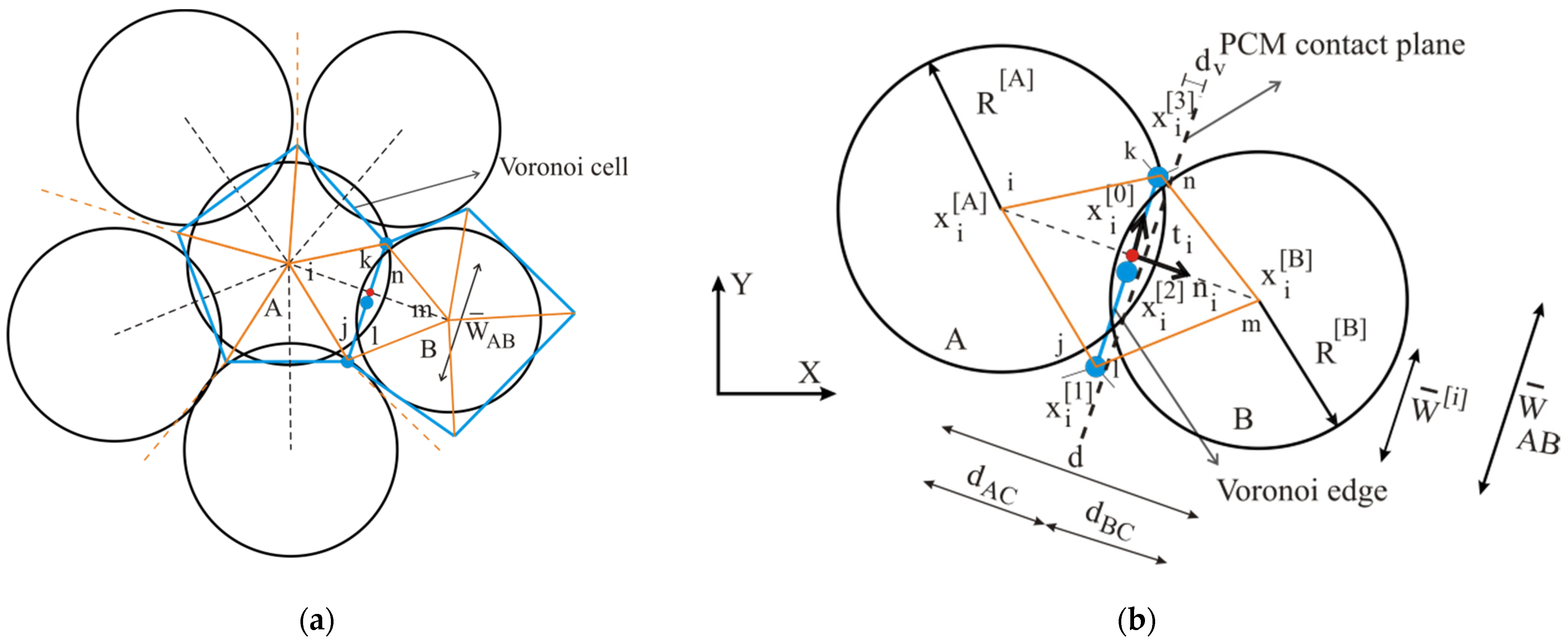
In the proposed contact model, like in the rigid contact model, the contact width and the contact location are defined by the Voronoi tessellation, Figure 1a. Similarly, the contact width corresponds to the length of the associated Voronoi cell edge, and the contact location is defined by the Voronoi cell edge [14]. The grains are considered to interact with neighbouring particles through the polygonal interface edges, Figure 1a.
The inner FE triangular mesh discretization of each Voronoi cell is defined by a triangulation of the Voronoi vertexes and the point corresponding to the particle centre of gravity, Figure 1. If required, it is also possible to add inner nodal points in order to refine the initial triangular FE mesh following a Delaunay triangulation scheme. Given that the rigid circular particles are only adopted to ease the contact interaction process, a scheme needs to be devised in order to transfer the contact forces from the contact locations to the corresponding nodal points of the FE mesh adopted in the grain discretization. The contact relative velocity also needs to be defined given the FE inner mesh nodal point velocities.
Like in the rigid contact version, the contact unit normal, n i , is defined given the particles centre of gravity and the inter-particle distance, d, Figure 1b:
n i = x i B x i A d
Similar to the rigid contact model, the contact overlap for the reference contact point, U n , and the reference contact point, x i [ 0 ] are defined by:
U n = R [ A ] + R [ B ] d
x i [ 0 ] = x i [ A ] + R [ A ] 1 2 U n d v n i
where d v is the distance along the contact normal between the point contact model (PCM) geometric contact plane of the two circular particles in contact and the adopted contact plane as defined by the corresponding Voronoi cell edge. If the Voronoi cell edge is located along the PCM contact plane ( d v = 0 ), the reference contact point location matches the contact location as defined in the traditional PCM contact model.
The position of each local contact point, x i J , is defined relatively to the reference local contact point, using the tangent vector to the Voronoi edge contact plane, t i [ J ] , and the contact distance in the tangent direction to the reference contact point, W ¯ [ J ] :
x i J = x i 0 + W ¯ [ J ] t i [ J ]
For the case of a three local contact point scheme as defined in Figure 1, the local contact point global coordinates are initially given by the Voronoi tessellation (the mid-point local contact location is given by averaging the Voronoi cell edge end point coordinates). The value of W ¯ [ J ] for each local contact point is then defined using Equation (11) given that the locations are known and taken directly from the Voronoi tessellation. The same procedure is adopted for other types of local contact point distributions. In [14], more details are given regarding the contact interaction.
In the proposed flexible contact model, the contact velocity is defined using the FE mesh discretization. As mentioned, the circular particles are rigidly associated with the inner nodal point that is initially located at the particle centre of gravity. The contact velocity of a given local contact point, which is the velocity of flexible particle B relative to flexible particle A, at the contact location is given by:
x ˙ i [ J ]       =   x ˙ i [ J ] B   x ˙ i [ J ] A =   N m . Δ m n l x ˙ i m . Δ m n l + N n . Δ m n l x ˙ i n . Δ m n l + N l . Δ m n l x ˙ i l . Δ m n l B N i . Δ i j k x ˙ i i . Δ i j k + N j . Δ i j k x ˙ i j . Δ i j k + N k . Δ i j k x ˙ i k . Δ i j k A
where N m . Δ m n l is the shape function value associated with nodal point “m” of the corresponding triangular finite element, Δ m n l , at the local contact point location x ˙ i [ J ] , and x ˙ i m . Δ m n l is the velocity of nodal point “m” of the corresponding triangular plane finite element, see 
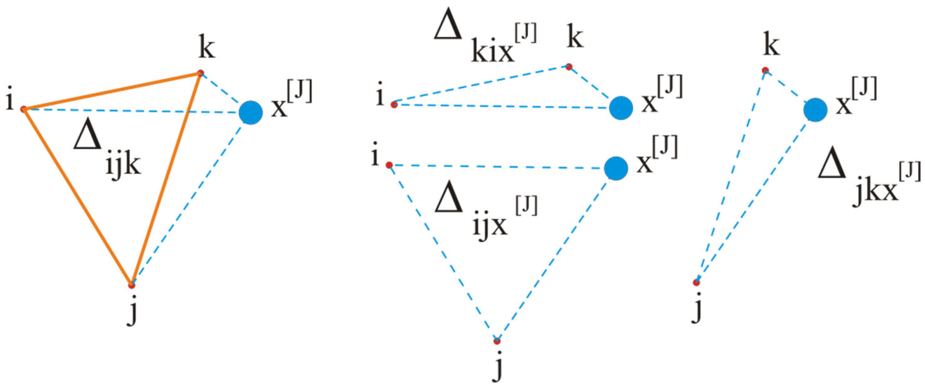
Figure 1b. The triangular shape functions’ values are defined in the traditional way according to the associated triangular areas (positive value clockwise), see Figure 2:
  N i . Δ i j k       =       Area Δ   j k x J / A r e a Δ   i j k N j . Δ i j k       =       A r e a Δ   k i x J / A r e a Δ   i j k N k . Δ i j k = A r e a Δ   i j x J / A r e a Δ   i j k
The contact displacement normal increment, Δ x J , N , stored as a scalar, and the contact displacement shear increment, Δ x i J , S , stored as a vector, are given by:
Δ x J , N =     x   i J Δ   t     n i
Δ x i J , S =     x   i J Δ   t     Δ x J , N n i
Given the normal and shear stiffnesses of the local contact point, the normal and shear forces increments are obtained following an incremental linear law:
Δ F i J , N = k n J   Δ x i J , N
Δ F i J , S = k s J   Δ x i J , S
The predicted normal and shear forces acting at the local contact point are then updated by applying the following equations:
F J , N . new = F J , N . old + Δ F i J , N
F i J , S . new = F i J , S . old + Δ F i J , S
Given the predicted normal and shear contact forces, the adopted constitutive model is applied, and, if the predicted forces do not satisfy the constitutive model, the necessary adjustments are carried out. The resultant contact force at the local contact point is then given by:
F J = F J , N   n i + F i J , S
The contact force at each local contact point is then transferred to the nodal points of the associated FE triangle given the nodal shape functions. For the triangular plane finite element associated with particle A and for the triangular element associated with particle B (Figure 1b), the local contact forces are distributed to each nodal point according to:
F i . Δ i j k c = F i . Δ i j k c F i [ C ] N i . Δ i j k
F m . Δ m n l c = F m . Δ m n l c + F i [ C ] N m . Δ m n l
The proposed flexible contact model can be transformed into a PCM-Flexible contact model if only one local contact point, located at the reference contact point, is adopted in the contact discretization, and if the distance of the adopted contact plane, located at the Voronoi cell edge, to the PCM contact plane is zero ( d v = 0 ).
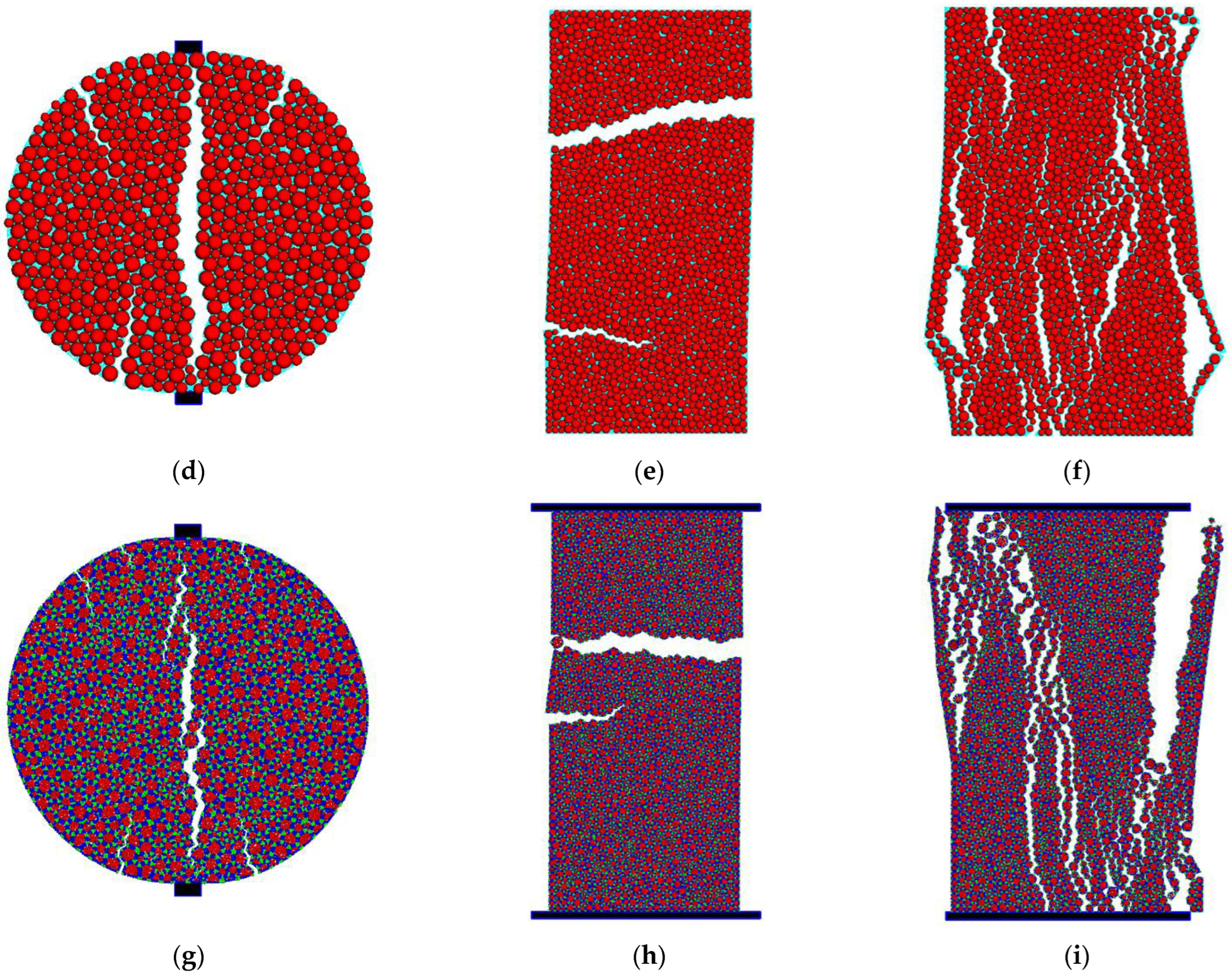
The proposed PM model also works under a large displacement hypothesis. If a new contact between two grains is found to occur, the Voronoi edge closest to the contact location is selected, in each grain, and the interaction follows the presented formulation. A similar contact interaction model, Pinball method, has been proposed by [25], where spheres are embedded in each finite element. This is obviously an approximation, but the examples presented show that it is a valid approach with clear computational advantages when compared with the usual deformable polygonal based DEM formulations that use much more complex interaction models [11,13,15]. If the grains had a more irregular shape, the geometry of each grain should be approximated by more than one circular particle [25] in order to better represent its outer boundaries [18].

2.4. Numerical Stability

When only a steady state solution is sought, a mass scaling algorithm is used in order to reduce the number of timesteps necessary to reach the desired solution. The nodal points masses are scaled so that the adopted centred-difference algorithm has a higher rate of convergence for a given loading step [22]. The nodal point scaled mass used in the calculations are set assuming a unit time increment, Δ t = 1 , given the nodal point associated stiffness at a given time through:
m scaled = 0.25   K t
An upper bound of the translation stiffness K t associated with the flexible contact model must be found at a given timestep:
K t = c = 1 N 2   j k n J + j k s J   N i . Δ i j k
where c = 1 N indicates a summation along the “N” contacts associated with nodal point “i”, k n J and k s J are the contact normal and shear stiffnesses, respectively, associated with local point j and N i . Δ i j k is the shape function associated with nodal point “i” of the triangular plane finite element associated with the proposed flexible contact.

2.5. Local Contact Stiffness and Local Contact Strength

In this work, the local contact normal and shear stiffnesses are given by:
k n J =   K n A c J
k s J = η   k n J
where A c J is the contact area associated with the local point j , K n is the normal stiffness adopted for the contact and η is the constant that relates the normal stiffness and the shear stiffness spring value. The total contact area is given by   A c = W ¯   t , where W ¯ is the contact interface width given by the Voronoi cell edge length, Figure 1b, and t is the out of plane thickness. The three local contact point scheme adopted in Figure 1b follows the Lobatto quadrature rule positioning: two local contact points at each edge end-point and one local contact point in the middle of the segment. The end-points have an associated local contact area of A c / 6 , and the mid-point has an associated contact area of 2 A c / 3 . The contact strength properties are defined given the maximum contact tensile stress, σ n . t , the maximum contact cohesion stress, τ, and the contact frictional term, μ c :
F n . max J = σ n . t   A c J
F s . max J = τ A c J + F n J   μ c = C max J + F n J   μ c
where F n . max J is the maximum contact local tensile strength, and F s . max J is the maximum local contact shear strength.

2.6. Local Contact Constitutive Model

Figure 3 shows the bilinear softening contact model adopted in the normal and shear directions. This contact model requires the definition of both the tensile fracture energy, G f . n , and the shear fracture energy, G f . s . The tensile damage value is defined based on the current local contact normal displacement ( D n J x n J ) Figure 3a, and the cohesion damage value is defined based on the current local contact shear displacement ( D s J x s J ), only the cohesion part is affected, Figure 3b. In each local contact point, the contact damage, D c J , is given by the sum of the tensile and shear contact damages. Given the current local contact damage, the local maximum tensile strength and maximum local cohesion strength are updated to:
F n . max J . Current = D c J   F n . max J
C max J . Current = D c J   C max J
A local crack is considered to occur when the maximum possible damage ( D c J = 1 ) is reached. At this stage, the local contact point is only considered to work under pure friction. A local contact crack is considered to be a tensile crack if the local contact was under a shear/tensile loading state when the maximum damage was reached. A local contact crack is considered to be a shear crack if the local contact was under a shear/compression loading state when the maximum damage was reached.
If the adopted contact fracture energy is equal to the energy corresponding to the elastic behaviour, the response of the bilinear model is the same as the response obtained using a traditional brittle Mohr–Coulomb model with tension cut-off. By using a bilinear softening model at the contact level, the fracture propagation occurs in a smoother and more controlled way than that numerically observed with a brittle model, allowing a less brittle response.

3. Simulation of Rock Specimens

3.1. Model Generation

In [14], a particle generation scheme was proposed which generates polygonal shaped particles based on the Laguerre Voronois using a weighted Delaunay triangulation of the circular particle gravity centres [26]. A Laguerre tessellation is preferred because it generates Voronois with edges closer to the traditional PCM geometric contact planes when considering two circular particles in contact. The initial circular particle assembly is created by first inserting the particles with half their radius, ensuring that the particles do not overlap with each other. Then, the particle real radius is adopted and a DEM cohesionless type solution is obtained, leading to a redistribution of the particle overlap throughout the assembly, Figure 4a.
The particle centres of gravity are then triangulated using a weighted Delaunay scheme and then the polygonal shaped particles are obtained given the Laguerre tessellation based on the weighted Delaunay triangulation, Figure 4b. The proposed flexible particle model further requires the generation of nodal points at the Laguerre cell vertexes and at the particle centre of gravity. A triangulation of the nodal points of each Laguerre cell is performed, Figure 4c. As previously mentioned, in the proposed flexible PM model, the contacts are adopted following the contact geometry of the Voronoi tessellation.
The adopted maximum particle diameter, Dmax, minimum particle diameter, Dmin, the radius distribution and the particles density, ρ, need to be defined taking into account the rock that is intended to be modelled. In the numerical simulations that were carried out, a porosity value of 10% was adopted in the definition of the initial number of particles to be inserted [2]. In this approach, the adopted porosity is not associated with the porosity of the rock to be modelled. Figure 4b,c show that a final compact assembly with no porosity is generated, both in the rigid and in the flexible PM models. Note that the outer grain contacts are exactly the same in the rigid and flexible PM models.

3.2. Model Parameters

The proposed flexible PM model requires the definition of seven elastic and strength parameters associated with the contacts. It also requires the definition of the Young’s modulus and the Poisson’s coefficient of the triangular finite elements adopted in the inner discretization of each Laguerre cell (polygonal particle).
The elastic response of the flexible PM model is related with the adopted contact elastic properties, contact normal stiffness, Kn, and the constant that relates the normal and the shear stiffness spring value (η), and with the continuum elastic properties adopted in the FE mesh. Nevertheless, as shown in Section 4.2, a flexible PM model that adopts the macroscopic rock elastic properties in the FE discretization does not require a previous calibration of the elastic contact properties.
The strength macroscopic response requires the definition of the maximum contact tensile stress, σn.t, the maximum contact cohesion stress, τ, the frictional term, μc, and both the contact tensile, G f . n , and the contact shear, G f . n , fracture energies. In the FE inner mesh discretization, an elastic behaviour is adopted.
Given that a direct relationship between contact properties and macroscopic properties is difficult to establish, the contact properties are traditionally defined through a calibration process in order to reproduce the known macroscopic material behaviour. In this work, a trial and error approach is adopted. The parametric study presented in Section 4.3.3 clearly shows the influence of each contact strength parameter in the predicted macroscopic response, which considerably reduces the burden of the trial and error procedure. In [15], a calibration procedure is proposed that adopts statistics techniques to ease the calibration procedure.

4. Biaxial and Brazilian Tests in a Granite Rock

4.1. Numerical Setup

The proposed flexible PM model is validated against known uniaxial, biaxial and Brazilian tests in a granite rock (Augig) [11,15]. The uniaxial tests, without lateral confinement pressure, and the biaxial tests with lateral confinement pressure are performed in samples with 80 mm × 160 mm. The Brazilian tests are performed on circles with a diameter of 80 mm. The simulations are performed in two dimensions; therefore, the particle assembly is considered to have 80 mm thickness. The course aggregate of Augig granite ranges from 3.0 to 7.0 mm [11]. In order to simulate this rock, both geometries were discretized with particles with a uniform diameter distribution ranging from 2.0 to 4.0 mm.
The uniaxial tests and the biaxial tests with lateral confinement have on average 1630 particles and 4627 contacts with three local points and the Brazilian tests have on average 640 particles and 1805 contacts with three local points. Figure 5a,b show the adopted rigid PM models following the contact approach proposed in [14], and Figure 5c,d shows the PM model following the proposed methodology. The flexible PM models have in addition 18,842 nodes and 25,003 triangular finite elements in the uniaxial and biaxial tests and 7376 nodes and 9784 finite elements in the Brazilian tests. On average, each grain that corresponds to a Voronoi cell is discretized with approximately 15 FE elements. In Figure 5, the particle radius is shown with a 50% reduction in order to make the adopted inner triangular plane element mesh visible.
In order to further validate and assess the computational costs associated with the proposed flexible PM model, particle assemblies where the grain deformability is defined through the inner contacts were also created, the uniaxial tests have on average 42,966 particles, and 23,977 contacts with one local point (Figure 5e). The Brazilian tests have on average 16,873 particles and 9438 contacts with one local point, Figure 5f. For the inner grain discretization, an average particle diameter of 0.06 mm was adopted, corresponding to an average of 26 inner particles per grain. As shown in Figure 5e,f, the inner particles have a different colour scheme: red corresponds to the interior particles, blue corresponds to the particles closer to the grain edges and green corresponds to the particles at the grain vertices. In the simulations that were carried out with a DEM model with inner discretization, two options were adopted, either the contact normal was defined in the usual way [2,14] or the contacts with the edge particles (blue particles in Figure 5e,f) had the contact normal given by the edge contact normal in order to reduce the natural roughness associated with the adopted particle discretization (a similar approach has been proposed in [6], known as the flat joint model).
The fact that an FE based model is adopted greatly eases the definition of boundary conditions, which are defined solely given the FE mesh. In the uniaxial tests, the nodal points at the upper and at the lower plate have their motion restrained in the vertical direction, a zero value at the lower plate and the imposed value at the upper plate, and the initial isotropic pressure is applied as an imposed stress at the boundary triangular FE edges.
In the rigid PM models, with or without the grain discretization with smaller particles, the boundary conditions are defined through vertical or horizontal plates that interact with the particle assembly through single point type contacts [2]. In order to simulate a flexible membrane, the horizontal plates are subdivided into 16 smaller plates that work independently and have their motion restrained along the horizontal plane, Figure 6.
In the biaxial tests with confinement, after setting the isotropic confinement stress, the nodal points (Flexible PM model) or the upper plate (rigid PM models) have their motion in the vertical direction given by a small downward velocity of 6.25 × 10⁻⁷ m/s, in order to simulate quasi-static conditions.
In the uniaxial compression test, the same value of downward velocity is adopted for the nodal points/upper rigid plate from the beginning of the simulation, and, in the uniaxial direct tensile test, the same value of velocity is adopted for the nodal points/upper rigid plate but in this case in the upward direction.
In the Brazilian tests, the quasi-static load is applied by giving a downward velocity, 6.25 × 10⁻⁷ m/s, to the upper rigid plate in all models. In the proposed flexible PM model, the upper rigid plate interacts with the neighbouring particles through a single point flexible contact model that follows the principles here described in Section 2.3 for a multiple flexible contact model. The lower plate rigid block has its motion restrained. In all tests, a local damping coefficient of 0.70 is adopted. The quasi-static plate velocity values are computed so that the measured macro-properties are not altered if the velocity value is further reduced.

4.2. Elastic Macroscopic Response

In a rigid PM model, the elastic macroscopic response is related to the adopted elastic contact properties, the normal stiffness and the normal to shear stiffness ratio. Given that in a rigid PM model it is not possible to devise analytical expressions for the elastic contact properties, it is necessary to calibrate them based on experimental results, usually using uniaxial compression tests.
With a flexible PM model, the elastic macroscopic response is related to the Young’s modulus and the Poisson’s coefficient of the triangular finite elements adopted in the inner discretization as well as with the adopted elastic contact properties. If the macroscopic rock properties are adopted in the inner grain triangular FE elements, then the adopted contact properties need to be high enough in order to ensure that the overall deformability is only associated with the FE mesh. In this approach, the contact properties can be understood as penalty values, and it is not necessary to perform a calibration of the elastic contact parameters. With a flexible PM model, it is also possible to adopt in the FE discretization, elastic properties closer to the mineral properties (e.g., quartz in a granitic rock). In this approach, the calibration procedure needs to be carried out in order to define the elastic contact properties that also contribute to the overall deformation.
In order to compare the performance of the proposed flexible PM model with the performance of a rigid PM model, several parametric studies were carried in order to assess the influence of the contact elastic parameters and of the elastic parameters adopted in the FE discretization on the macroscopic elastic response. In all presented models, the adopted reference normal contact stiffness is the value that gives the best agreement of the numerical model with the known experimental values for an Augig ganite rock that is used as comparison. For the flexible PM models based on FE discretization, two different values of the Young’s modulus were adopted, a value of 25.8 GPa similar to the Young’s modulus of Augig granite and a value of 51.6 GPa on the order of magnitude of the Young’s modulus of the minerals usually present in a granite rock. A Poisson’s coefficient of 0.23 similar to the known Poisson´s coefficient of an Augig rock was adopted in both flexible models.
Figure 7 shows the influence of the contact deformability parameters ( K n and η ) on the elastic macroscopic properties of the particle assembly ( E and υ ) for all the adopted PM models. As shown in Figure 7a,b, in the rigid PM model, both contact elastic parameters influence the macroscopic Young’s modulus and Poisson’s coefficient. It can be seen that macroscopic Young’s modulus is more sensitive to the shear to normal stiffness ratio for higher contact normal stiffness values. Figure 5b shows that, in the rigid PM model, the macroscopic Poisson’s coefficient is mainly influenced by the shear to normal stiffness relationship ( η ). The dashed line represents the known values for an Augig rock (E = 23.8 GPa, u = 0.23).
For the flexible PM model where the Augig rock macroscopic elastic properties are adopted in the triangular FE elements, Figure 7c,d, it can be seen that the macroscopic values are mostly influenced by the FE adopted properties. In this approach, the adopted contact elastic properties only need to be chosen sufficiently high in order for the particle deformability to be solely associated with the inner FE discretization. As shown in Figure 7c,d, the shear to normal stiffness relationship ( η ) has a negligible influence in the macroscopic elastic response.
When the elastic properties adopted for the triangular FE elements are within the order of magnitude of the minerals that are present in a granite rock, (e.g., quartz), Figure 7e,f, it can be seen that the macroscopic values are mostly influenced by the adopted FE elastic properties, but in this approach the contact properties also influence the macroscopic properties, mostly the macroscopic Poisson’s coefficient.
In summary, a flexible particle model with the FE properties close to the rock to be modelled does not require a previous calibration procedure for the contact properties, which is a clear advantage when compared with a rigid PM model. In this approach, the shear to normal stiffness ratio can be set to any given value in between 0.2 to 0.6 [15,24].

4.3. Strength Macroscopic Response

4.3.1. FEM versus DEM Based Deformability

In order to assess the influence of taking into account the grain deformability and to compare the proposed FEM based PM model with a DEM based flexible model through contact discretization, several uniaxial tests were carried out. Table 1 presents the adopted elastic contact properties, which are the best fit values for the adopted PM models, and Table 2 presents the contact strength properties that were considered to be a best fit for a rigid PM model with a uniform radius between 2.0 mm and 6.0 mm. Note that, in this work, a uniform particle radius distribution between 2.0 mm to 4.0 mm was adopted. The adopted inner discretization FEM triangles elastic properties match the macroscopic Augig properties and the inner contact properties (DEM flexible model) were calibrated in order to also match the hard rock macroscopic elastic properties. The Augig granite macro-properties are presented in Table 3 [11,15]. Figure 8 shows the axial stress–displacement response under compression, including the contact damage evolution, for the proposed FEM based deformable PM model and for two DEM based deformable PM models, one where the unit contact normal at the grain boundaries is given by the Voronoi cell edge contact normal (DEM-un), similar to the model flat joint model [6], and another model where the contact normal is defined using the usual unit normal formula (DEM) [1,2] similar to the model flat joint model [22]. It can be seen that the proposed FEM based flexible PM model predicts, for similar contact strength properties, results within the boundaries of the values predicted with the DEM based flexible models where the grain deformation is due to the inner contacts.
The presented results show that, if smaller particles are adopted in the discretization of the inner grains, there is an associated interlock that reduces the brittle behaviour even if the Voronoi edge unit normal is adopted for contact interaction. The post-peak response is also influenced by the adopted numerical damping and boundary conditions; nevertheless, it is clearly shown that, for similar conditions, a rigid PM model with grain deformability given by the inner contacts leads to a less brittle response. If a Voronoi tessellation is adopted to describe the rock grain distribution, the ideal is to adopt a flexible PM model as proposed here or to adopt polygonal type interactions [11,16].
Figure 9 shows the axial stress–displacement response under compression, including the contact damage evolution for the proposed FEM based flexible PM model and for a rigid PM model with similar strength properties [14]. It can be seen that the consideration of the particle deformability with the proposed flexible PM model does not change the post-peak brittle behaviour that is predicted with a rigid PM model, as also observed experimentally in hard rock. For a brittle model, the grain deformability consideration does not affect the predicted compression strength peak value, whereas, for a bilinear contact model, the consideration of the grain deformability leads to an increase in the peak compressive strength. Figure 9 also shows that the rigid PM model predicts a stress–strain response with two clear distinct slopes for a zero-confinement pressure (uniaxial compression). With a bilinear softening contact model, the change in the inclination of the stress-deformation curve is less pronounced when compared with a brittle model, but it is still noticeable. This change in the stress/deformation slope occurs due to the damage evolution that occurs for low compression values. When compared with the rigid PM model, the onset of damage evolution occurs in the flexible PM model for higher compression values, Figure 9. With polygonal flexible based models, this change in slope is also not predicted [15].
Table 4 presents, for the uniaxial tests and for the Brazilian tests, the computational execution times for the rigid PM model, for the proposed flexible FEM based PM model and for the flexible DEM based model (inner contacts). The computational run times associated with the proposed flexible FEM based model are higher than those associated with the rigid PM model, with an average multiplying factor of around 8.0, for the uniaxial and biaxial tests and an average multiplying fact of around 5.0 for the Brazilian tests. Table 4 also shows that the computation run times associated with the flexible DEM model (inner contacts) are around three times higher than the proposed FEM based PM model in the uniaxial tests and around 1.2 times higher in the Brazilian tests.
It is important to note that, when compared with polygonal FEM flexible PM models [13,15], the proposed flexible FEM based PM model has lower computational requirements due to the fact that the contact interaction is still performed taking into account the circular grain geometry. Because the contact location and unit normal are defined in an approximate way, the proposed model is not as accurate as the polygonal based models in terms of contact interaction. Nevertheless, the final failure patterns presented in Figure 10 show that reasonable final failure patterns are predicted with the proposed approximate flexible PM model in good agreement with the failure pattern predicted with a rigid PM model and with a flexible PM model based on the grain discretization with smaller particles.

4.3.2. Strength Envelope

Figure 11 shows the Hoek–Brown failure criterion applied to the Augig granite experimental values [11,15], the values predicted adopting the proposed flexible FEM based PM model for two different inner triangles Young’s modulus (25.8 GPa and 51.6 GPa), and the results predicted with a rigid PM model [14]. Brittle and bilinear softening contact laws were adopted in each PM model. The contact strength parameters that were found to give a best fit agreement with Augig hard rock with a rigid PM model were adopted [14] (Table 2). The larger markers presented in Figure 11 represent the predicted tensile strength with a Brazilian test, and the smaller markers represent the predicted tensile strength through uniaxial testing.
Figure 11a shows that, for a brittle constitutive law, the flexible PM model with an inner discretization Young modulus of 25.8 GPa predicts a friction angle higher than that predicted with a rigid PM model. All PM models with a brittle contact model predict an indirect tensile strength lower than the direct tensile strength. With a brittle model, the response predicted with the flexible PM model (E = 51.6 GPa) is closer to the response predicted with a rigid PM model than to the response predicted with a flexible PM model (E = 25.8 GPa).
For a bilinear constitutive law, the flexible PM model with an inner discretization Young’s modulus of 25.8 GPa predicts a friction angle higher than that predicted with a rigid PM model [14], Figure 11b. All PM models following a bilinear contact model predict an indirect tensile strength higher than the direct tensile strength, but the flexible based PM models predict higher indirect to direct tensile ratio for the same set of contact parameters. As shown in Figure 11b, the response predicted with a flexible PM model (E = 51.6 GPa) is between the response predicted with a rigid PM model and the response predicted with a flexible PM model (E = 25.8 MPa). This result is closer to the expected because, as the inner triangles stiffness is increased, the macroscopic results should converge to those predicted with a rigid PM model.

4.3.3. Influence of Strength Contact Parameters

In order to further assess the particle deformability influence and to compare the proposed FEM based PM model with a rigid PM model, several simulations were carried out for different contact strength values. The simulations were carried out assuming a constant maximum contact tensile stress of σn.t = 11.50 MPa and four τ/σn.t relationships, τ/σn.t = 1, 2, 3 and 4. The same contact frictional term μc = 0.5 was adopted in all tests. Three different contact fracture energies under tension (Gf.n) were adopted. In all cases, a shear (Gf.s) fracture energy 31.5 times higher than the adopted tensile fracture energy was adopted. The adopted contact tensile fracture energy varied between 66.1 N/m (Gf1), 33.1 N/m (Gf2) and 16.5 N/m (Gf3). The adopted contact strength properties are presented in Table 5.
Figure 12a–g show the predicted numerical responses for the proposed flexible PM model (F) and, for the rigid PM model (R), namely the compression strength, the friction angle, the cohesion, the direct tensile strength, the indirect tensile strength, the direct tensile strength to indirect tensile ratio, and the compression to indirect tensile strength ratio. Figure 12a shows that, for similar properties, the flexible PM model predicts higher compression strength values; it is also shown that higher fracture energies and higher contact shear to tensile ratio lead to higher compression strength in both PM models. With the flexible PM model, the contact fracture energy has a higher influence on the macroscopic response.
Figure 12b shows the predicted macroscopic friction angle. It shows that both PM models predict a higher friction angle for a lower shear to tensile strength ratio. As shown, the influence of the adopted contact fracture energy is less noticeable in the flexible PM model. Regarding the predicted macroscopic cohesion response, Figure 12c, it is shown that a higher shear to tensile contact strength favors an increase in the cohesion. Figure 12c also shows that a flexible PM model predicts higher cohesion values than a rigid PM model for similar contact strength properties.
Figure 12d, which represents the macroscopic direct tensile strength, shows that, for similar contact properties, the flexible PM model predicts higher strength values. Figure 12d also shows that the influence of the contact shear to tensile strength is negligible in both the flexible and rigid PM models. As shown, higher contact fracture energy leads to higher macroscopic strength. Figure 12e show that both the ratio of shear to tensile strength and the adopted fracture energies influence the predicted indirect tensile strength response on both PM models. The flexible PM model for similar contact properties predicts higher indirect tensile strength macroscopic response.
Regarding the direct tensile to indirect tensile strength ratio, a flexible PM model is shown to always predict lower ratios, Figure 12f, when compared with a rigid PM model for similar properties. As shown in Figure 12f for a shear to tensile strength ratio of 2, the flexible PM model predicts ratios lower than 1 for all the adopted tensile fracture energy values. In rock, the indirect tensile strength is usually higher than the direct tensile strength value [27,28]. Several factors can explain this difference, namely the fact that in the Brazilian test the induced stress state close to the plates is rather complex with a clearly defined compressive stress zone, and also the fact that the final crack pattern is not perfectly plane. As presented in Figure 12f, a ratio of direct to indirect tensile strength ratio lower than 1 is more difficult to be predicted with a rigid PM model. As pointed out in [14], only contact models that consider bilinear softening contact laws are able to predict direct tensile to indirect tensile strength ratios closer to 1.0.
Figure 12g shows the predicted compression strength to direct tensile strength ratio. As shown, a flexible PM model predicts higher ratios of compressive to tensile strength when compared with a rigid PM model. Figure 12g also shows that a higher shear to tensile contact strength leads to a higher compression to tensile strength in both models.
Additionally, several simulations were carried out in order to assess the influence of the contact friction term. With this purpose, three different contact friction values were adopted, 0.2, 0.5 and 0.8. In all studies, a contact tensile fracture energy of 33.1 N/m and a shear (Gf.s) fracture energy 31.5 times higher than the adopted tensile fracture energy were adopted. Two τ/σn.t relationships, τ/σn.t = 1 and τ/σn.t = 3 were considered, assuming a constant maximum contact tensile stress of σn.t = 11.50 MPa. The adopted contact strength properties are presented in Table 6.
Figure 13a shows that, in both PM models, an increase in the contact friction term leads to an increase in the predicted macroscopic compressive strength. As shown in Figure 13a when compared with a rigid PM model, a flexible PM model is more influenced by the adopted contacted friction term for both adopted shear to tensile contact strength ratios.
Figure 13b shows that the predicted macroscopic friction angle is influenced by the adopted contact frictional term in both models, almost showing a linear relationship. Regarding the predicted macroscopic cohesion response, Figure 13c shows the predicted macroscopic cohesion. As shown, the contact friction effect on the macroscopic cohesion response is less noticeable in the flexible PM model than in the rigid PM model, especially for a shear to tensile strength ratio of 3.
Figure 13d shows that, in both PM models, the contact friction term has a negligible effect in the macroscopic direct tensile strength. Similarly, the effect of the contact friction term in the predicted macroscopic indirect tensile strength is also negligible, Figure 13e in both PM models. As expected, the contact friction term influence on the direct to indirect tensile strength ratio is also negligible (Figure 13f).
Figure 13g shows the predicted compression strength to a direct tensile strength ratio. As shown, when compared with a rigid PM, the flexible PM model predictions are more influenced by the adopted contact frictional term.

4.3.4. Calibrated Response (Bilinear Constitutive Model)

A trial and error estimating procedure was carried out in order to find the contact strength parameters that allow the flexible PM model to have an excellent agreement with an Augig Rock experimental values [11,15]. Before carrying out a trial and error procedure, it is important to perform a sensitive analysis as presented in Section 4.3.3 in order to understand the influence that each contact strength parameter has on the macroscopic response. Usually, the trial and error approach starts by setting a given shear to tensile contact strength ratio, and then finding the tensile contact strength value that predicts an indirect tensile strength closer to that desired. Then, the contact fracture energy is slightly tuned so that the PM model is also able to predict the compressive strength. Finally, the contact friction term is tuned in such a way that the PM model is able to predict the failure envelope. If the predicted numerical response is not closer to the experimental results, the previous steps are repeated for a different shear to tensile strength ratio. More complex calibration procedures have been proposed [15], but the trial and error procedure, if one knows how the contact strength parameters influence the macroscopic response, can still be carried out even if one has to deal with five contact strength parameters (tensile, cohesion, frictional term, tensile and shear fracture energies).
Figure 14 shows the Hoek–Brown failure criterion applied to the Augig granite experimental values [11,15] and the values predicted adopting the proposed flexible FEM based PM model (E = 25.8 GPa). As shown, the flexible PM is able to predict an indirect tensile strength higher than the predicted tensile strength. Table 7 presents the contact strength best fit values for a bilinear contact constitutive model. Comparing the presented values with the values presented in Table 2, it can be seen that a flexible PM model when compared with a rigid PM model requires a lower tensile contact strength and a lower fracture energy and a slightly higher shear to tensile strength ratio. The frictional term has a similar value.
Figure 15 presents the predicted uniaxial compression response and the predicted response for a confinement stress of 4.0 MPa. Also shown are the experimental response and the numerical response obtained with a flexible polygonal PM model that also adopts a softening branch under tensile loading and shear [15]. The proposed numerical flexible PM model is in good agreement with the predicted numerical response [15], but it can be seen that PM models, either rigid or flexible, still need to be further developed in order to match the Augig granite macroscopic response.

5. Discussion and Conclusions

PM models, either rigid or flexible, should be able to predict the rock complex macroscopic response under any state of stress (compressive, tensile, and shear) with the same set of parameters [15]. For this reason, several enhancements have been proposed which have introduced more complex geometries, grain deformability and more complex contact models.
A flexible PM model is proposed that considers the particle deformability by adopting in each grain, Voronoi Cell, an inner finite element mesh. The contact interaction is an extension of the rigid contact model proposed in [14], which keeps the contact interaction simplicity and the reduced computational costs characteristic of circular rigid particle models. When compared with polygonal based flexible models [15], the proposed model, by keeping the highly efficient contact detection procedures associated with circular shapes, has lower associated computational costs. It is shown that the proposed flexible PM model has a computational cost higher than a similar rigid PM model (eight times higher), but three times lower than the computational cost associated with an all-particle PM model, where the grain deformability is due to the grain discretization, like the models proposed in [5,7]. Furthermore, it is shown that the all-particle PM models has an inherit grain interlock, even if a flat joint contact approach is adopted, which may lead to a more ductile post-peak response, contrary to that observed in hard rock, which is closer to the more brittle response predicted with the proposed flexible PM model and with a similar rigid PM model [14].
A flexible PM model greatly eases the process of setting the boundary conditions (confinement stress, imposed displacement boundaries) and as shown does not require the calibration of the elastic contact properties if the inner discretization finite elements Young’s modulus match the hard rock macroscopic value. Nevertheless, the rigid PM elastic calibration procedure, even if based on a trial and error procedure, is quite straightforward to be performed.
Given that the studied PM models have exactly the same particle arrangements and outer grain contacts, the performance of the proposed flexible PM models could be straightforwardly compared with the performance of a rigid PM model [14]. In this way, it was possible to assess the influence of the grain deformability on the macroscopic response, which is original to PM studies. The results presented show that a PM model should reproduce the real grain deformability in order to be as accurate as possible and in order for the contact strength parameters to be closer to real material contact parameters, as the grain deformability is an important feature that influences the macroscopic response. When compared with a rigid PM model, the main disadvantage of a flexible PM model is the associated increase in the computational costs, which the presented PM model tries to remain as low possible by keeping the circular particle interactions’ simplicity.
The parametric results presented here show that the influence of the contact strength parameters on the macroscopic response differs if the PM model is rigid or flexible. As shown, the flexible PM model, when compared with a rigid PM model, requires a smaller value of contact tensile fracture energy in order to predict a correct direct to indirect tensile strength ratio. This means that the contact fracture energy in a rigid PM model has to be artificially increased in order to compensate the fact that the stress distribution may not be correct as the particles are rigid. It is also shown that a flexible PM model also requires a softening contact model in order to predict a correct direct tensile to indirect tensile strength ratio.
Rigid PM models with an associated low computational cost are suitable for large scale studies, but, as shown in this paper, the proposed flexible PM model is a more accurate competitive alternative.

Author Contributions

Conceptualization, N.M.A., M.L.B.F. and S.O.; methodology, N.M.A. and M.L.B.F.; software, N.M.A. and S.O.; validation, N.M.A., M.L.B.F. and S.O.; writing—original draft preparation, N.M.A. and M.L.B.F.; writing—review and editing, M.L.B.F., N.M.A. and S.O.; supervision, N.M.A.; project administration, N.M.A. and M.L.B.F. All authors have read and agreed to the published version of the manuscript.

Funding

This research received no external funding.

Acknowledgments

The study presented here is part of the ongoing project “DAMFA-Cutting-edge solutions for sustainable assessment of concrete dam foundations” carried out jointly by LNEC and FCT/UNL, with the main purpose of developing a numerical multiphysical integrated tool for the sustainable assessment of concrete dam foundations, taking into account the interaction between mechanical, hydraulic and thermal behaviours.

Conflicts of Interest

The authors declare no conflict of interest.

References

  1. Potyondy, D.; Cundall, P.; Lee, C. Modelling rock using bonded assemblies of circular particles. In Proceedings of the 2nd North American Rock Mechanics Symposium, Montreal, QC, Canada, 19–21 June 1996; pp. 1937–1944. [Google Scholar]
  2. Potyondy, D.O.; Cundall, P.A. A bonded-particle model for rock. Int. J. Rock Mech. Min. 2004, 41, 1329–1364. [Google Scholar] [CrossRef]
  3. Cho, N.; Martin, C.D.; Sego, D. A clumped particle model for rock. Int. J. Rock Mech. Min. 2004, 44, 997–1010. [Google Scholar] [CrossRef]
  4. Ye, Y.; Thoeni, K.; Zeng, Y.; Buzzi, O.; Giacomini, A. A novel 3D clumped particle method to simulate the complex behaviour of rock. Int. J. Rock Mech. Min. 2019, 120, 1–16. [Google Scholar] [CrossRef]
  5. Potyondy, D.O. A grain-based model for rock approaching the true microstructure. In Proceedings of the Rock Mechanics in the Nordic Countries, Kingsber, Norway, 9–12 June 2010. [Google Scholar]
  6. Potyondy, D.O. A flat-jointed bonded-particle material for hard rock. In Proceedings of the 46th US Rock Mechanics/Geomechanics Symposium American Rock Mechanics Association, Chicago, IL, USA, 24–27 June 2012. [Google Scholar]
  7. Zhou, J.; Lan, H.; Zhang, L.; Yang, D.; Song, J.; Wang, S. Novel grain-based model for simulation of brittle failure of Alxa porphyritic granite. Eng. Geol. 2019, 251, 100–114. [Google Scholar] [CrossRef]
  8. Wang, Y.; Tonon, F. Modeling Lac du Bonnet granite using a discrete element model. Int. J. Rock Mech. Min. Sci. 2009, 46, 1124–1135. [Google Scholar] [CrossRef]
  9. Azevedo, N.M.; Lemos, J.V. A 3D generalized rigid particle contact model for rock fracture. Eng. Comput. 2013, 30, 277–300. [Google Scholar] [CrossRef] [Green Version]
  10. Scholtès, L.; Donzé, F.-V. A DEM model for soft and hard rocks: Role of grain interlocking on strength. J. Mech. Phys. Solids 2013, 61, 352–369. [Google Scholar] [CrossRef]
  11. Kazerani, T.; Zhao, J. Micromechanical parameters in bonded particle method for modelling of brittle material failure. Int. J. Numer. Anal. Methods Géoméch. 2010, 34, 1877–1895. [Google Scholar] [CrossRef]
  12. Lan, H.; Martin, C.; Hu, B. Effect of heterogeneity of brittle rock on micromechanical extensile behaviour during compression loading. J. Geophys. Res. 2010, 115, 1–14. [Google Scholar] [CrossRef]
  13. Itasca UDEC. Distinct-Element Modeling of JOINTED and Blocky Material in 2D, version 7.0; Itasca Consulting Group Inc.: Minneapolis, MN, USA, 2018. [Google Scholar]
  14. Azevedo, N.M.; Candeias, M.; Gouveia, F. A Rigid Particle Model for Rock Fracture Following the Voronoi Tessellation of the Grain Structure: Formulation and Validation. Rock Mech. Rock Eng. 2015, 48, 535–557. [Google Scholar] [CrossRef]
  15. Kazerani, T.; Zhao, J. A Microstructure-Based Model to Characterize Micromechanical Parameters Controlling Compressive and Tensile Failure in Crystallized Rock. Rock Mech. Rock Eng. 2014, 47, 435–452. [Google Scholar] [CrossRef]
  16. Gao, F.; Stead, D. The application of a modified Voronoi logic to brittle fracture modelling at the laboratory and field scale. Int. J. Rock Mech. Min. 2014, 68, 1–14. [Google Scholar] [CrossRef]
  17. Ghazvinian, E.; Diederichs, M.; Quey, R. 3D random Voronoi grain-based models for simulation of brittle rock damage and fabric-guided micro-fracturing. J. Rock Mech. Geotech. Eng. 2014, 6, 506–521. [Google Scholar] [CrossRef] [Green Version]
  18. Li, X.F.; Li, H.B.; Zhao, J. 3D polycrystalline discrete element method (3PDEM) for simulation of crack initiation and propagation in granular rock. Comput. Geotech. 2017, 90, 96–112. [Google Scholar] [CrossRef]
  19. Zhou, W.; Ji, X.; Ma, G.; Chen, Y. FDEM Simulation of Rocks with Microstructure Generated by Voronoi Grain-Based Model with Particle Growth. Rock Mech. Rock Eng. 2020, 53, 1909–1921. [Google Scholar] [CrossRef]
  20. Tang, P.; Chen, G.-Q.; Huang, R.-Q.; Wang, D. Effect of the number of coplanar rock bridges on the shear strength and stability of slopes with the same discontinuity persistence. Bull. Eng. Geol. Environ. 2021, 80, 3675–3691. [Google Scholar] [CrossRef]
  21. Le, H.-K.; Huang, W.-C.; Chien, C.-C. Exploring micromechanical behaviors of soft rock joints through physical and DEM modeling. Bull. Eng. Geol. Environ. 2021, 80, 2433–2446. [Google Scholar] [CrossRef]
  22. Underwood, P. Dynamic relaxation. In Computation Methods for Transient Analysis; Belytschko, T., Hughes, T., Eds.; Elsevier Science Publishers B.V.: Oxford, UK, 1983; pp. 245–265. [Google Scholar]
  23. Cundall, P. Distinct element models for rock and soil structure. In Analytical and Computational Methods in Engineering Rock Mechanics; Brown, E.T., Ed.; Allen & Unwin: London, UK, 1987; Chapter 4; pp. 129–163. [Google Scholar]
  24. Lemos, J.V.; Cundall, P. Earthquake analysis of concrete gravity dams on jointed rock foundations. In Distinct Element Modelling in Geomechanics; A.A. Balkema: Rotterdam, The Netherlands, 1999; pp. 117–143. [Google Scholar]
  25. Belytschko, T.; Yeh, I.S. The splitting pinball method for contact-impact problems. Comput. Method Appl. Mech. Eng. 1993, 105, 375–393. [Google Scholar] [CrossRef]
  26. Okabe, A.; Boots, B.; Sugihara, K. Spatial Tessellations: Concepts and Applications of Voronoi Diagrams; John Wiley & Sons: Hoboken, NJ, USA, 1992. [Google Scholar]
  27. Klanphumeesri, S. Direct Tension Tests of Rock Specimens. Master’s Thesis, Suranaree University of Technology, Nakhon Ratchasima, Thailand, 2010. [Google Scholar]
  28. Erarslan, N.; Williams, D. Experimental, numerical and analytical studies on tensile strength of rocks. Int. J. Rock Mech. Min. 2012, 49, 21–30. [Google Scholar] [CrossRef]
Figure 1. Flexible contact model for a discretization with three local contact points including triangular finite element mesh: (a) contact width and location at the Voronoi cell; (b) three local contact point scheme.
Geotechnics 02 00026 g001
Figure 2. Flexible contact model triangular shape functions at local contact point x i [ J ] .
Geotechnics 02 00026 g002
Figure 3. Bilinear softening contact model: (a) normal direction; (b) shear direction.
Geotechnics 02 00026 g003
Figure 4. From the grain structure to the flexible contact model: (a) initial grain structure; (b) rigid contact model based on the Voronoi tessellation [14]; (c) propose flexible particle model, including the inner FE mesh.
Geotechnics 02 00026 g004
Figure 5. Particle assemblies: (a) uniaxial and biaxial tests (Rigid PM model); (b) Brazilian test (Rigid PM model); (c) uniaxial and biaxial tests (proposed flexible PM model); (d) Brazilian test (proposed flexible PM model); (e) uniaxial and biaxial tests (Rigid PM-inner contacts) and (f) Brazilian test (Rigid PM-inner contacts).
Geotechnics 02 00026 g005aGeotechnics 02 00026 g005b
Figure 6. Rigid PM models boundary conditions through rigid plates: (a) rigid PM model; (b) grain deformability through inner discretization (Rigid PM-inner contacts).
Geotechnics 02 00026 g006
Figure 7. Influence of the contact deformability parameters ( K n and η ) on the elastic macroscopic properties of the particle assembly ( E and υ ) for the rigid contact PM model [14] and for the proposed flexible FEM PM model for two different finite element Young´s modulus values: (a) Rigid PM model [14]: Macroscopic Young’s modulus for varying η n = 1.08 × 10⁴ GPa/m; (b) Rigid PM model [14]: Macroscopic Poisson’s coefficient for varying η -Kn = 1.08 × 10⁴ GPa/; (c) Flexible PM model: Macroscopic Young’s modulus for varying η -Kn = 18.00 × 10⁴ GPa/m, E = 25.8 GPa; (d) Flexible PM model: Macroscopic Poisson’s coefficient for varying η -Kn = 18.00 × 10⁴ GPa/m, E = 25.8 GPa; (e) Flexible PM model: Macroscopic Young’s modulus for varying η-Kn = 2.06 × 10⁴ GPa/m, E = 51.6 GPa; (f) Flexible PM model: Macroscopic Poisson’s coefficient for varying η-Kn = 2.06 × 10⁴ GPa/m, E = 51.6 GPa.
Geotechnics 02 00026 g007
Figure 8. Axial stress–displacement response under uniaxial compression-proposed flexible PM models and DEM-inner contacts): (a) brittle model; (b) bilinear softening model.
Geotechnics 02 00026 g008
Figure 9. Axial stress–displacement response under uniaxial compression–proposed flexible PM models and rigid PM model: (a) brittle model; (b) bilinear softening model.
Geotechnics 02 00026 g009
Figure 10. Particle assemblies: (a) Brazilian test (Rigid PM model); (b) uniaxial tensile test (Rigid PM model); (c) uniaxial compression test (Rigid PM model); (d) Brazilian test (proposed flexible PM model); (e) uniaxial tensile test (proposed flexible PM model); (f) uniaxial compression test (Proposed flexible PM model); (g) Brazilian test (DEM-Flexible); (h) uniaxial tensile test (DEM-Flexible) and (i) uniaxial compression test.
Geotechnics 02 00026 g010aGeotechnics 02 00026 g010b
Figure 11. Strength envelope: Hoek–Brown failure criterion adopted from [11], Rigid model [14] and proposed flexible FEM based particle model: (a) brittle contact constitutive law; (b) bilinear softening contact constitutive law.
Geotechnics 02 00026 g011
Figure 12. Effect of τ/σn.t and fracture energy contact properties on macroscopic response, Rigid (R) and Flexible (F) numerical predicted response: (a) compression strength; (b) friction angle; (c) cohesion; (d) direct tensile strength; (e) indirect tensile strength; (f) direct to indirect tensile strength ratio and (g) compression to direct tensile strength ratio.
Geotechnics 02 00026 g012aGeotechnics 02 00026 g012b
Figure 13. Contact friction properties influence on macroscopic response, Rigid (R) and Flexible (F) numerical predicted response: (a) compression strength; (b) friction angle; (c) cohesion; (d) direct tensile strength; (e) indirect tensile strength; (f) direct to indirect tensile strength ratio and (g) compression to direct tensile strength ratio.
Geotechnics 02 00026 g013aGeotechnics 02 00026 g013b
Figure 14. Strength envelope: Hoek–Brown failure criterion adopted from [11,15] and calibrated flexible FEM based particle model (bilinear constitutive model).
Geotechnics 02 00026 g014
Figure 15. Axial stress-axial strain response under different confinement pressures numerical and experimental response adapted from [15] and proposed calibrated FEM base PM model: (a) uniaxial compression; (b) 4 MPa confinement.
Geotechnics 02 00026 g015
Table 1. Contact elastic properties for the particle models.
Type of Contact K n ( GPa / m ) η
Rigid PM [14]1.08 × 1040.28
Flexible PM FEM (E = 25.8)18.00 × 1040.28
Flexible PM DEM-inner contacts (E = 25.8)4.90 × 1040.30
Flexible PM FEM (E = 51.6)2.06 × 1040.28
Table 2. Contact strength properties for the particle models [14].
Type of Contact σ n . c ( MPa ) τ c ( MPa ) μ c G f . n ( N / m ) G f . s ( N / m )
Brittle13.7048.800.40(-)(-)
Bilinear11.533.250.566.12078.6
Table 3. Augig granite macro-properties [11,15].
Type of Contact E ν σ c ( MPa ) σ t . i n d ( MPa ) c ϕ (°)
Brittle25.80.23122.18.821.053.0
Table 4. Execution times (hours) for the completion of 1,000,000 calculation cycles.
ModelUniaxial CompressionBrazilian Test
Rigid PM [14]1.140.75
Proposed Flexible PM (FEM)9.293.59
Flexible PM (DEM-inner contacts)28.154.34
Table 5. Strength properties for the particle models: Influence of contact strength.
Case σ n . c ( MPa ) τ c ( MPa ) μ c G f . n ( N / m ) G f . s ( N / m )
Gf111.511.50.566.12082.2
23.0
34.5
46.0
Gf211.533.11042.7
23.0
34.5
46.0
Gf311.516.5519.8
23.0
34.5
46.0
Table 6. Strength properties for the particle models: Influence of contact friction.
Case σ n . c ( MPa ) τ c ( MPa ) μ c G f . n ( N / m ) G f . s ( N / m )
τ/σn.t=111.511.50.233.11042.7
0.5
0.8
τ/σn.t=311.534.50.2
0.5
0.8
Table 7. Contact strength properties for the proposed particle models.
Type of Contact σ n . c ( MPa ) τ c ( MPa ) μ c G f . n ( N / m ) G f . s ( N / m )
Bilinear8.529.750.4020.0800.0
Publisher’s Note: MDPI stays neutral with regard to jurisdictional claims in published maps and institutional affiliations.

