1. Introduction
The screw Driving Sounding (SDS) test is a relatively new in-situ test for soil characterisation, recently developed in Japan [
1]. This test consists of a machine drilling a rod into the ground, with a screw point attached, in seven steps of monotonic loading. In this test, the load increases at every complete rotation of the rod, with the load steps set at 0.25, 0.38, 0.50, 0.63, 0.75, 0.88, and 1 kN. The speed of rotation is constant at 25 rpm. The measured parameters in the test are: the applied torque on the rod (
T), the amount of penetration (
L), the penetration velocity (
V), and the number of rotations (
N) of the rod. These parameters are measured at every complete rotation of the rod. After each 25 cm penetration, the rod is lifted by 1 cm and then rotated to measure the rod friction. The machine used and the procedure for doing the SDS test are shown in
Figure 1. Further details of the SDS tests are presented elsewhere [
1,
2,
3].
To estimate the soil properties for use in geotechnical design from the measured SDS data, it is necessary to develop correlations. Some theoretical and empirical relationships between the SDS data and various soil properties have been developed. For example, soil classification charts based on SDS-derived parameters have been developed [
3,
4] and further refined with the availability of more data [
5]. Correlations with parameters obtained from more popular in-situ tests, such as the N-value from standard penetration tests and tip resistance, sleeve friction, and soil behaviour type index from cone penetration tests, have been proposed [
3,
6]. Procedures to predict the liquefaction potential of sandy soils have also been formulated and validated with the data observed in Christchurch according to the Canterbury Earthquake Sequence [
4,
7,
8]. Moreover, procedures to estimate other index properties of soils, such as fines contents, plasticity index, and shear strengths, have been recommended [
9,
10,
11].
Although several empirical correlations have been developed to estimate soil parameters based on the data obtained from SDS tests, numerical simulation of the SDS drilling procedure can be helpful to better understand the ground response and to identify potentially important parameters that could contribute to the results obtained. As a result, the accuracy of the empirical predictions can be improved.
In recent years, developments in high-speed computing have reduced the cost of analysis and rendered the finite element method a powerful tool for solving geotechnical engineering problems. Different types of constitutive models for soils can be implemented in finite element (FE) methods, such as the Mohr-Coulomb plasticity, extended Drucker-Prager plasticity, modified Drucker-Prager/cap model, and clay plasticity. Various boundary conditions, initial stress states, void ratio distributions, or soil saturation can be specified. Any combinations of loads, such as concentrated, gravity, or distributed, can be applied in the models. Prescribed displacements can be defined, and, depending on the problem, different contact conditions between the parts can be introduced. However, complex problems involving large deformations are usually difficult to solve using the classical FE method. Large deformations can lead to significant mesh distortions and contact problems. The frictional contact between soil and structure may become complicated.
In the FE method, the most common mesh approach used to model regions undergoing small deformation is the Lagrangian approach; however, this is not suitable for cases where excessive element distortion is expected. In such cases, the Eulerian meshing approach is more appropriate. Initially developed for fluid-structure interaction, the coupled Eulerian-Lagrangian (CEL) method has been formulated to combine the advantages of the Lagrangian and Eulerian formulations. That is, the CEL method allows the user to selectively mesh the analysis of components according to the physics being modelled, with the Eulerian technique used in regions undergoing large deformations and the remaining using the conventional Lagrangian technique. The CEL method has found many applications in simulating geotechnical problems, such as in laboratory element testing [
12], penetration tests in clays [
13], ground improvement applications [
14], and water-soil interaction problems [
15], among others.
In this paper, the CEL method, implemented through the FE software Abaqus, has been used to simulate and analyse the drilling process involved in performing the SDS test in a sandy deposit with specified relative density and effective overburden pressure. The simulation analyses various parameters recorded during a typical SDS test, from which the measured maximum torque is considered. Based on the simulation results, a chart was established to correlate the measured torque with the internal friction angle for various effective overburden stresses. To validate the chart, the required friction angle for a specified effective vertical stress and a monitored maximum torque are compared with the friction angle obtained from laboratory tests performed on samples taken from several sites in Christchurch, NZ, adjacent to the locations of the SDS test. The results show that the CEL FE framework can model complex physical processes encountered during the screw point penetration. In addition, the developed chart can be used to estimate the friction angle of the sandy soil based on the SDS-measured torque at a given depth.
2. Estimation of Rod Friction during SDS
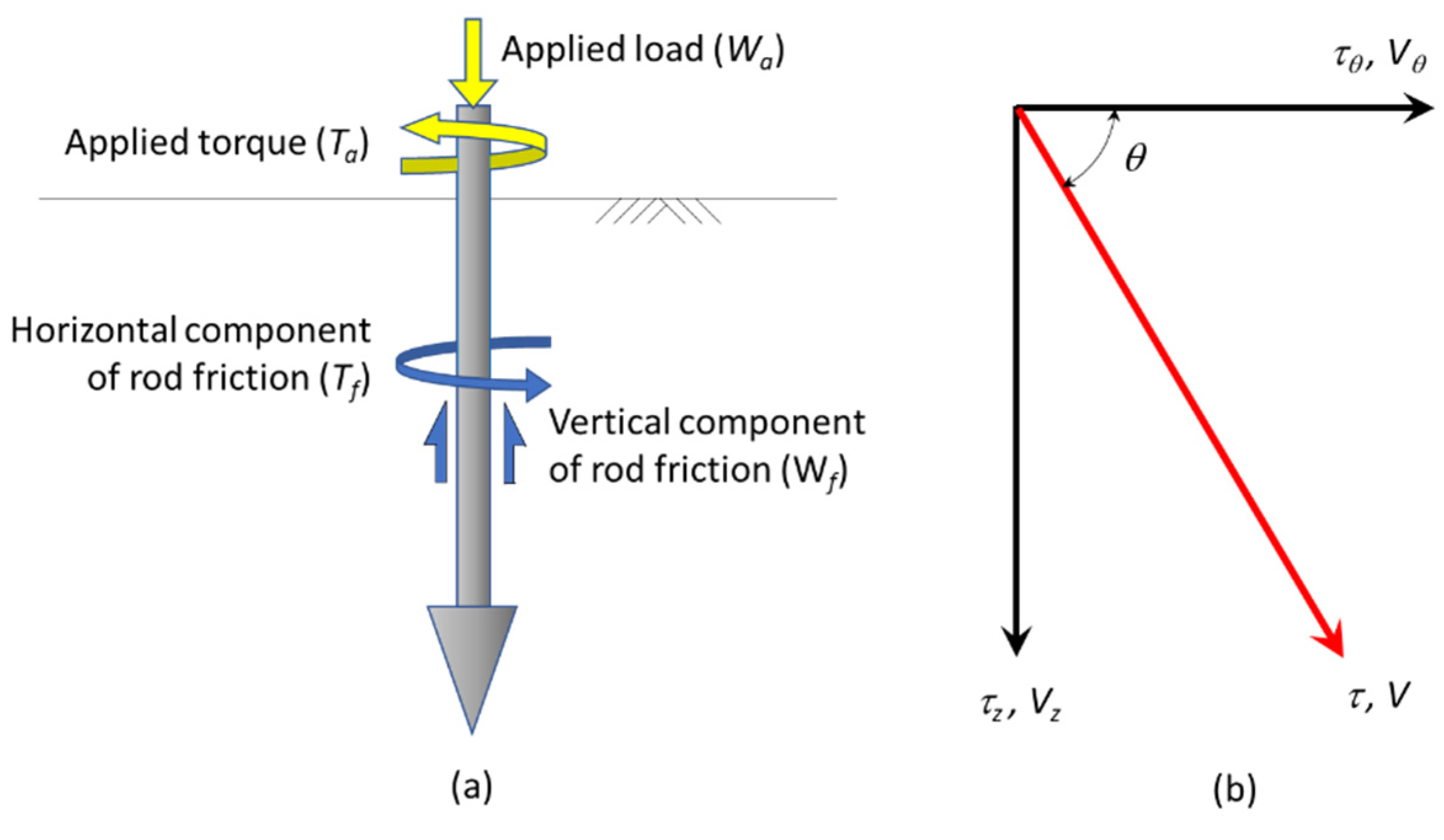
Due to the effects of rod friction on the measured torque and load, while the rod is penetrated during the SDs test, the measured load and torque required for penetration are more than the ones applied at the screw point, located at the tip of the rod. The rod friction can be divided into a vertical component (
and a horizontal component (
) as the rod rotates and penetrates the ground [
1].
Figure 2 shows the concept of measuring rod friction.
The load (
) and torque (
) applied by the SDS equipment are defined as follows:
where
and
are the load and torque (both corrected for friction) at the screw point, respectively. The maximum shear stress acting on the rod body is computed as follows:
where
is the torque resisting the rod friction measured at the end of a loading set,
is the radius of the rod, and
is the amount of penetration. If the direction of rotation velocity (
) and the penetration velocity (
) are equal to those of the horizontal shear stress (
) and the vertical shear stress (
) on the rod surface, respectively, then the equations for stresses can be given as follows:
The angle
can be derived from the ratio between
and
Vz, i.e.,
. When Equation (3) is substituted into Equations (4) and (5), the vertical and horizontal components of the rod friction are obtained as [
1]:
3. Coupled Eulerian-Lagrangian (CEL) Analysis
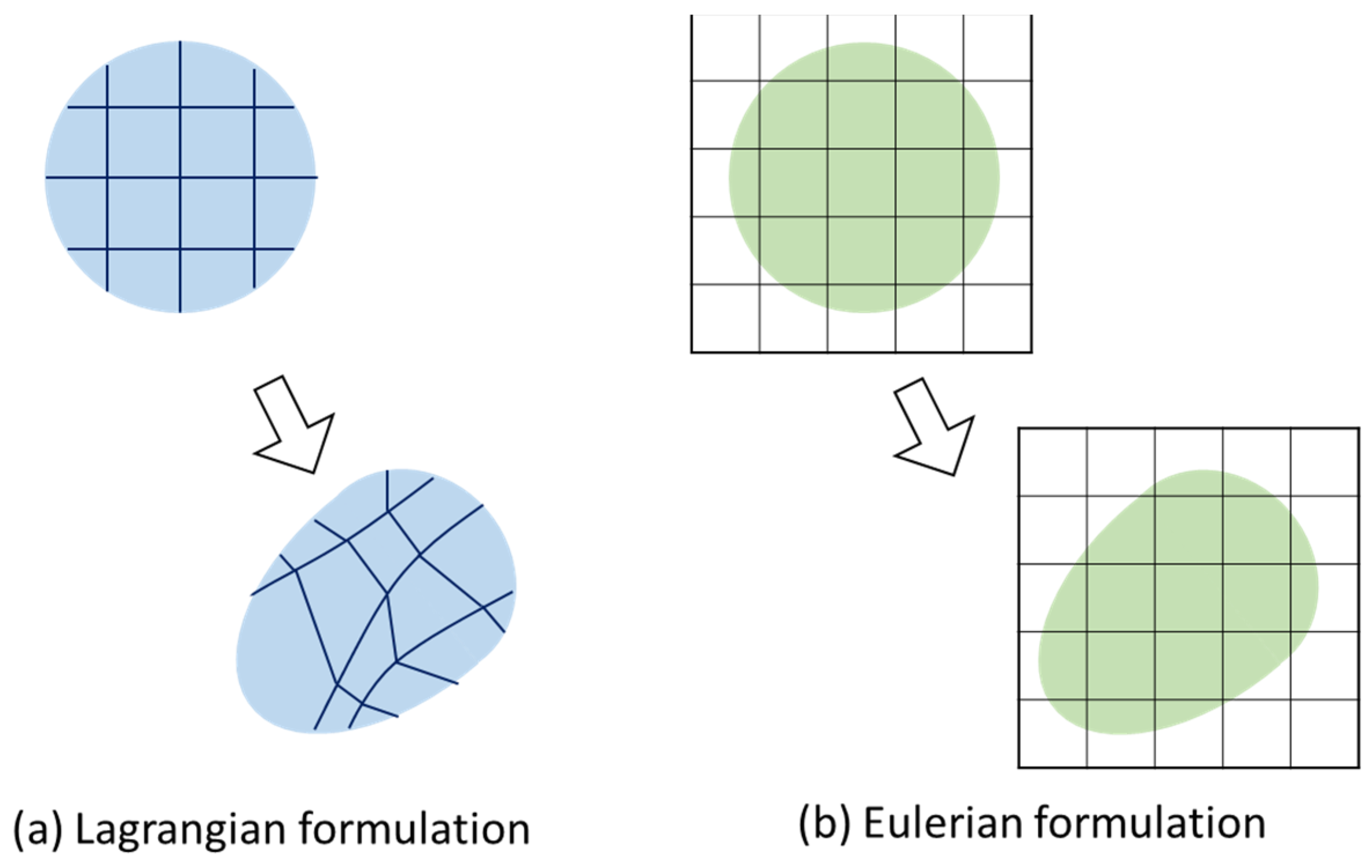
When a meshed (discretised) continuum deforms, the positions of the small continuum elements change with time. These positions can be described as functions of time in two ways: the Lagrangian description and the Eulerian description (
Figure 3). The Lagrangian method describes the movement of the continuum as a function of the material coordinates and time. In this formulation method, the nodes of the Lagrangian mesh and the material move together. Therefore, the interface between the two parts can be precisely tracked. However, using the Lagrangian method, large deformations may cause severe element distortions. The Lagrangian approach is a material description usually applied in solid mechanics.
On the other hand, the Eulerian method specifies the movement of the continuum as a function of the spatial coordinate and time. In this method, a Eulerian reference mesh is fixed and remains undistorted, and the materials can freely flow through the mesh. The advantage of this method is that no element distortion happens; however, the interface between two parts cannot be described as precisely as when the Lagrangian formulation is used [
16,
17]. The Eulerian method is a field description usually applied in fluid mechanics.
Coupled Eulerian-Lagrangian (CEL) analyses are those whereby Eulerian material can interact with Lagrangian material through Eulerian-Lagrangian contact. This method attempts to capture the advantages of both Lagrangian and Eulerian approaches [
18]. This method is suitable for simulating problems involving large deformations, such as cone penetration tests (CPT) or pile penetration problems [
19]. In this method, the movement of the Eulerian material is tracked and defined as it moves through the mesh by computing its Eulerian volume fraction (EVF) within each element. The portion of a filled element with the material is represented as a fraction. An EVF equal to 1 represents an element fully filled with the material, while an EVF equal to 0 means the element is free of any material. It is also possible that the Eulerian elements simultaneously contain more than one material. If the sum of the EVF in an element is less than one, the remaining part of the element is automatically filled with “void” material, which does not have mass, strength, or stiffness [
20]. Contact between Eulerian and Lagrangian materials can only be defined using a general contact, where contact constraints are enforced with the penalty method. A general contact has a simple definition of contact with very few restrictions on the types of involved surfaces. It uses sophisticated tracking algorithms to ensure that proper contact conditions are enforced efficiently [
21].
4. Modelling Screw Point Penetration into the Ground
4.1. Geometry and Modelling Steps
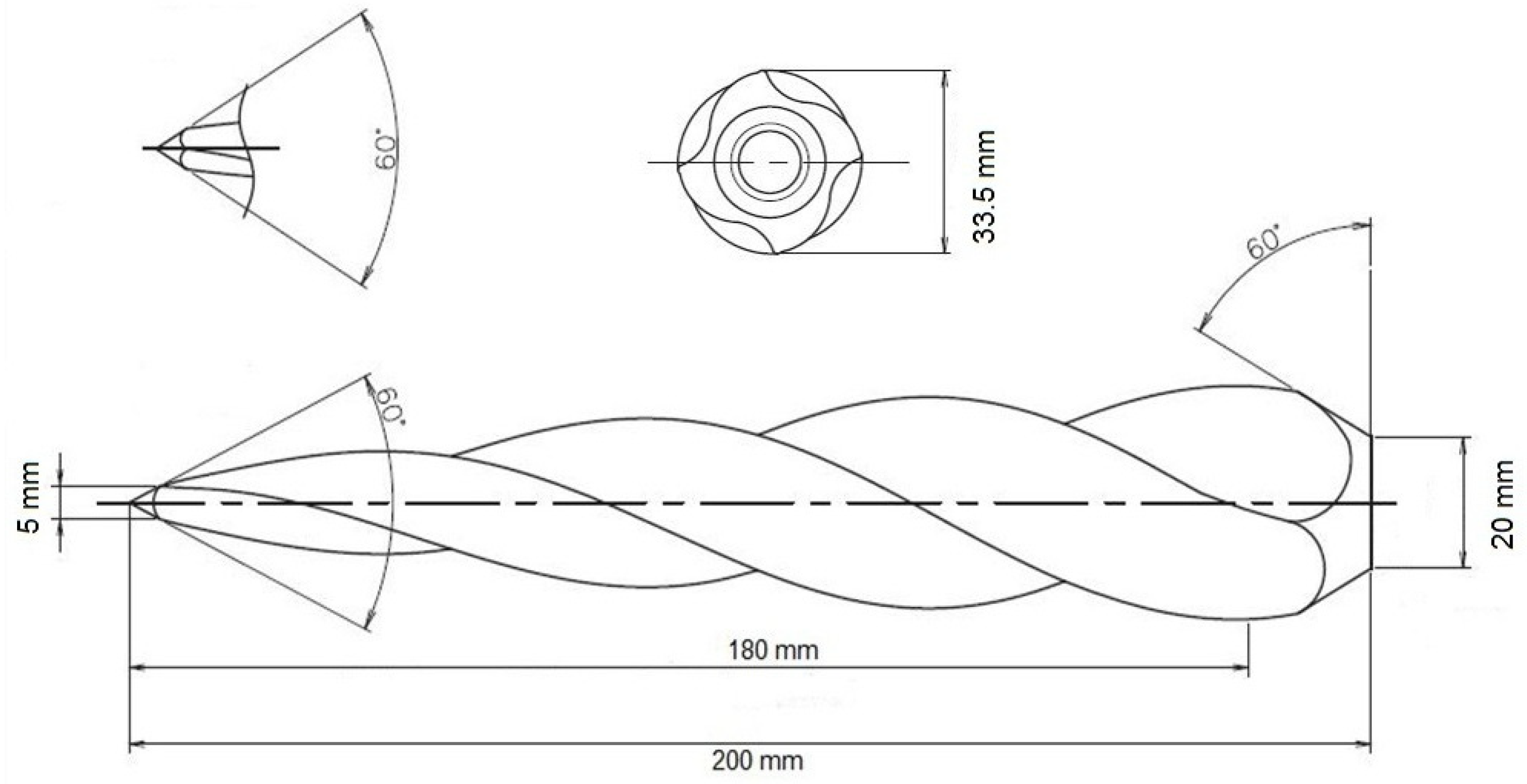
Due to the helical shape of the screw point, a three-dimensional modelling approach needs to be adopted when applying the CEL method. The maximum diameter of the screw point was 33.5 mm with a length of 200 mm. The diameter of the screw point at the tip was 5 mm. The drilling tool was modelled as a rigid body because it was assumed that the deformation of the screw point was negligible compared to the large deformation of the soil. The screw point had a general diameter of about 33.5 mm, and the drill rod was about 20 mm. The screw point was precisely modelled with AutoCAD (version 20.0) software and then imported into the Abaqus software.
Figure 4 shows the schematic view of the screw point and its dimensions, while
Figure 5 shows the screw point drawn with AutoCAD.
The soil was modelled with Eulerian elements, and its shape was cylindrical, with a diameter of 500 mm and a height of 750 mm. The boundary of the model was sufficiently far enough that it did not influence the results. This was validated by analysing the stress bulb created around the screw point that did not touch the boundaries. On the top of the soil model, a void area of 2 cm thickness was provided so that the top surface of the soil could move into this free space due to the effects of soil dilation and distortion generated during the drilling process. The entire Eulerian area comprises 98,592 eight-noded three-dimensional elements (with a reduced integration scheme). These Eulerian elements were used to discretise the soil body (Abaqus element type: EC3D8R). The discretised model is shown in
Figure 6.
The drilling rod penetrated the soil at a constant speed of rotation (clockwise from the top view). It was assumed that the soil response did not depend on the penetration velocity; that is, the soil behaviour was assumed to be strain rate-independent, at least within the depth considered. The rotational velocity was taken as 25 rpm (the same as the actual field test). At the first stage of the model, the screw point was placed at the surface of the model, and initial gravity loads were applied. Then, prior to applying the rod rotation, the entire length of the screw point was pushed into the soil to simulate the subsequent drilling process after completing one set of 25 cm of penetration. In the next stage, following the stage in which the screw point was embedded into the soil, both the load and rotation were applied to the drilling rod. The vertical load and rotation were applied simultaneously with the overburden pressure at the surface of the model as a distributed load. The reaction moment in the screw point along the vertical axis was recorded during the second step by monitoring the value on a node defined as the reference point on top of the rod (as shown in
Figure 6). The vertical and horizontal displacements of the model ground were constrained at the bottom, while the horizontal displacements were restrained at the sides.
4.2. Constitutive Model
Various constitutive models for capturing soil behaviour have been developed and reported in the literature, e.g., [
22,
23,
24]. The models vary in terms of complexity in that some are quite simple, while others are complex and require many input parameters. In this study, to describe the behaviour of sand, a simple elastic perfectly-plastic constitutive model based on the Mohr-Coulomb yield criterion is used [
25]. This model has been adopted because of its simplicity in its formulation and in terms of the input parameters needed and the required computational time. Here, the elastic modulus describes the elastic behaviour of sand, and the friction and dilation angles define the plastic deformation. In this study, only clean sand was simulated, and therefore no cohesion was defined. The dilatancy of the soil was described using a non-associated flow rule.
4.3. Interface Modelling
Abaqus/Explicit provides two algorithms for modelling contact and interaction problems: the general contact algorithm and the contact pair algorithm. In the CEL method, only the general contact algorithm based on the penalty contact method can be used to define the contact between the Eulerian material and Lagrangian material.
In the penalty contact method, seeds are created on the Lagrangian element edges and faces, while anchor points are created on the Eulerian material surface. The penalty method approximates hard pressure–overclosure behaviour. This method allows slight penetration of the Eulerian material into the Lagrangian domain.
The general contact algorithm in Abaqus/Explicit is specified as part of the model or history definition of the model. It allows very simple definitions of contact with very few restrictions on the types of surfaces involved, and it uses sophisticated tracking algorithms to ensure that proper contact conditions are enforced efficiently.
Currently, the finite-sliding formulation is the only available tracking approach for general contact. The finite-sliding formulation allows arbitrary motion of the surface, such as separation, large sliding, and rotation, and it is well-suited to simulate highly nonlinear processes with large deformation.
The frictional sliding at the interface between the screw point and soil is modelled with the Coulomb friction model. In this simulation, the normal contact is chosen as hard contact and does not include any friction and thermal interaction in the normal direction. The hard contact implies no limit to the magnitude of contact pressure that can be transmitted when the surfaces are in contact.
For the tangential contact, the coefficient of interface friction (
) is defined as:
where
is the angle of interface friction. Durgunoglu and Mitchell [
26,
27] recommended using
= 0.5 for most penetrometers, where
is the peak angle of internal friction.
4.4. Initial Stress
In this study, the SDS simulation was performed only for the last loading step, i.e., where the total applied load was 1 kN. The required torque for one complete rotation of the screw point was recorded. The simulation was performed at five levels of effective vertical stresses, up to a maximum of 110 kPa, which were applied as a distributed load at the surface of the model. The coefficient of lateral earth pressure,
, is defined as follows:
4.5. Dilation Angle
The dilation angle,
, for the non-associated flow rule model was calculated by adopting the ‘saw blade’ model of dilatancy [
28,
29], as expressed by Equation (10):
where
is the residual angle of internal friction (in degrees). In this study, a constant value of
was chosen based on test results for silica sands [
28]. Ideally, the dilation angle (
) should be modelled as a function of the soil strain; however, it was assumed to be a constant value in order to simplify the problem. To examine the similarity between Christchurch sand and silica sand, consolidated drained triaxial tests were conducted on reconstituted samples from 3 different sites in Christchurch (NZ) located at Avondale Rd, Pages Rd, and Bideford Pl. Sieve analysis was performed on the samples based on New Zealand Standards NZS 4402.2.8 [
30]; all the samples were found to be sand with fines content,
FC, of less than 5%. The relative densities of the in-situ samples were estimated with available CPT data based on the method proposed by Idriss & Boulanger [
31]. In determining the dry density of the samples, the maximum and minimum densities of the samples were measured in the laboratory-based on New Zealand Standards NZS 4402.4.2 [
32]. Triaxial samples were remoulded to their in-situ densities in accordance with the methodology described by NZS 4402.6.2 [
33]. The measured peak and residual friction angles of the samples at an effective confining pressure of 100 kPa are summarised in
Table 1. As seen from the table, the behaviour of Christchurch sand is almost similar to Silica sand, with all three samples having critical state friction angles of 33°. Therefore, the assumed critical state friction angle for the simulation is reasonable.
4.6. Young’s Modulus
The stress-strain behaviour of any type of soil depends on many factors, such as relative density, water content, fabric/structure, drainage conditions, duration of loading, and strain state, among others. By conducting laboratory tests on samples under conditions similar to the field conditions, it is possible to consider most of these factors. This concept simplifies the procedures required to determine the soil’s stress-strain relationships and avoids explicitly incorporating the complex factors in the constitutive models. Duncan and Chang [
18] developed a practical stress-strain relationship to determine the elastic modulus (
). The proposed formulation is as follows:
where
is the failure ratio (=
),
is the stress condition at failure,
is the cohesion,
is the peak friction angle, and
is the asymptotic value of stress. The value of
is always less than unity. For a number of different types of soils, the value of
has been found to lie between 0.75 and 1.
was calculated as 0.9(
) based on the work of Byrne et al. [
34], where
for silica sand.
is the modulus number for primary loading,
is the modulus exponent,
is the atmospheric pressure (100 kPa),
is the major principal stress, and
is the minor principal stress.
was chosen as a function of
in accordance with trends observed by Duncan and Chang [
23]. A typical range of
for dense sand to
for loose sand was used based on the behaviour observed by Duncan and Chang [
23].
Table 2 summarises all the parameters used in this analysis.
4.7. Effect of Mesh Size
The mesh convergence study was conducted by analysing two FE models: the original model comprising 98,592 elements and a finer mesh model (that had 136,896 elements). The effect of mesh size on the reaction moment (see
Section 5.3) was analysed. It was found that the difference in the reaction moments at the end of one complete rotation and the trend between the results of these two FE models are negligible; these demonstrate the convergence of the original FE mesh. It can be said that making the mesh size finer would simply increase the computational time, with no significant effect on the accuracy.
Figure 7 shows the reaction moments calculated using the two different mesh sizes. As shown in the figure, the value of the recorded reaction moment (torque) is slightly different during the rotation process. Still, the reaction moments from both models reach almost the same value at the end of the one rotation (i.e., end of 2.4 s). As discussed later, the basis of this analysis is to use the value of
, which occurs at the end of a complete rotation; the difference between the torques calculated during the process can be ignored.
5. Results and Discussion
5.1. Deformed Mesh
As discussed in the previous sections, the penetration during one complete rotation of the screw point in the last loading step is modelled with the CEL method. Conventional FE models often lead to large element distortions due to large deformations of the soil. However, through the CEL method, it was shown that the drilling process does not cause element distortion due to large deformation. While the CEL method is used, the Eulerian mesh, which represents the soil, does not move, and the Lagrangian part can penetrate it. Therefore, there is no element distortion when the soil experiences large deformations.
5.2. Stress Distribution
Figure 8 shows the distributions of the vertical and horizontal stress in the soil for 60 kPa overburden pressure and angle of friction of 34° after one complete rotation of the screw point. The advancement forces of any screw or drilling tool are produced by its wings (edges), which convert the applied torque into a vertical force during the penetration by pushing the surrounding materials upward and sideways. The resultant concentration of stresses can be observed in the contour plots. The stresses in the area around the edges of the screw point have the highest values due to the concentration of stresses in the location where shearing occurs.
5.3. Reaction Moments
As mentioned earlier, one complete rotation of the screw point is simulated with the application of a vertical load of 1 kN at the top of the rod (which is the maximum applied load) and a predefined constant rotational speed of 25 rpm. The reaction torque (moment), which is caused by the interaction between the screw point (Lagrangian part) and the soil (Eulerian part), is recorded along the vertical axis (on a node defined on top of the rod), which is conceptually similar to the measured torque in the SDS test during the operation.
Figure 8 shows the result of the analysis as smoothed measured reaction moment for the soil with a friction angle of 34° and a vertical effective stress of 110 kPa. In the SDS test, the maximum value of torque (
) at each step of loading is measured, and the value for the vertical load of 1 kN is taken and compared with the results of the simulations. The reaction moment was measured for the different combinations of friction angle and effective vertical stress listed in
Table 2; the results are discussed below (refer to
Section 5.4 and
Section 5.5).
As shown in
Figure 9, the analysis indicates that the amount of reaction moment (torque) increases with time and, after one-half turn (1.2 s), the slope of the curve decreases, which means that the torque increases at a slower rate. At the beginning of the rotation, the screw point is filled with soil. As the screw point starts rotating, it pushes the soil sideways. Hence, in the second half turn (1.2 s to 2.4 s), the initial soil around the screw point is pushed away completely, and the measured torque during the second stage changes less. The measured torque at the end of one complete rotation is considered as
(maximum torque), similar to the actual SDS test.
5.4. Effect of Friction Angle
Next, the effect of the friction angle on the reaction moment was studied. Three different friction angles were used in the simulation. All the simulations were performed on cohesionless soil.
Figure 10 shows the effect of increasing friction angle for a given effective overburden pressure on the reaction moment. As expected, increasing the friction angle, i.e., corresponding to denser sand, the value of the torque at the end of one complete rotation increases. It is also found that the rate of change of the torque with the friction angle is more when the overburden pressure is higher, i.e., at a higher overburden pressure, the torque increases more rapidly with friction angle. This can be explained by the fact that a high overburden pressure prevents the soil from dilating; hence, for the dense sands (dilation angles of 1° and 3°), a larger torque is required for penetration. Moreover, an increase in the effective overburden pressure increases the shear resistance of the soil. As a result, when the overburden pressure increases, the change in the required torque with increasing friction angle becomes larger.
5.5. Effect of Overburden Pressure
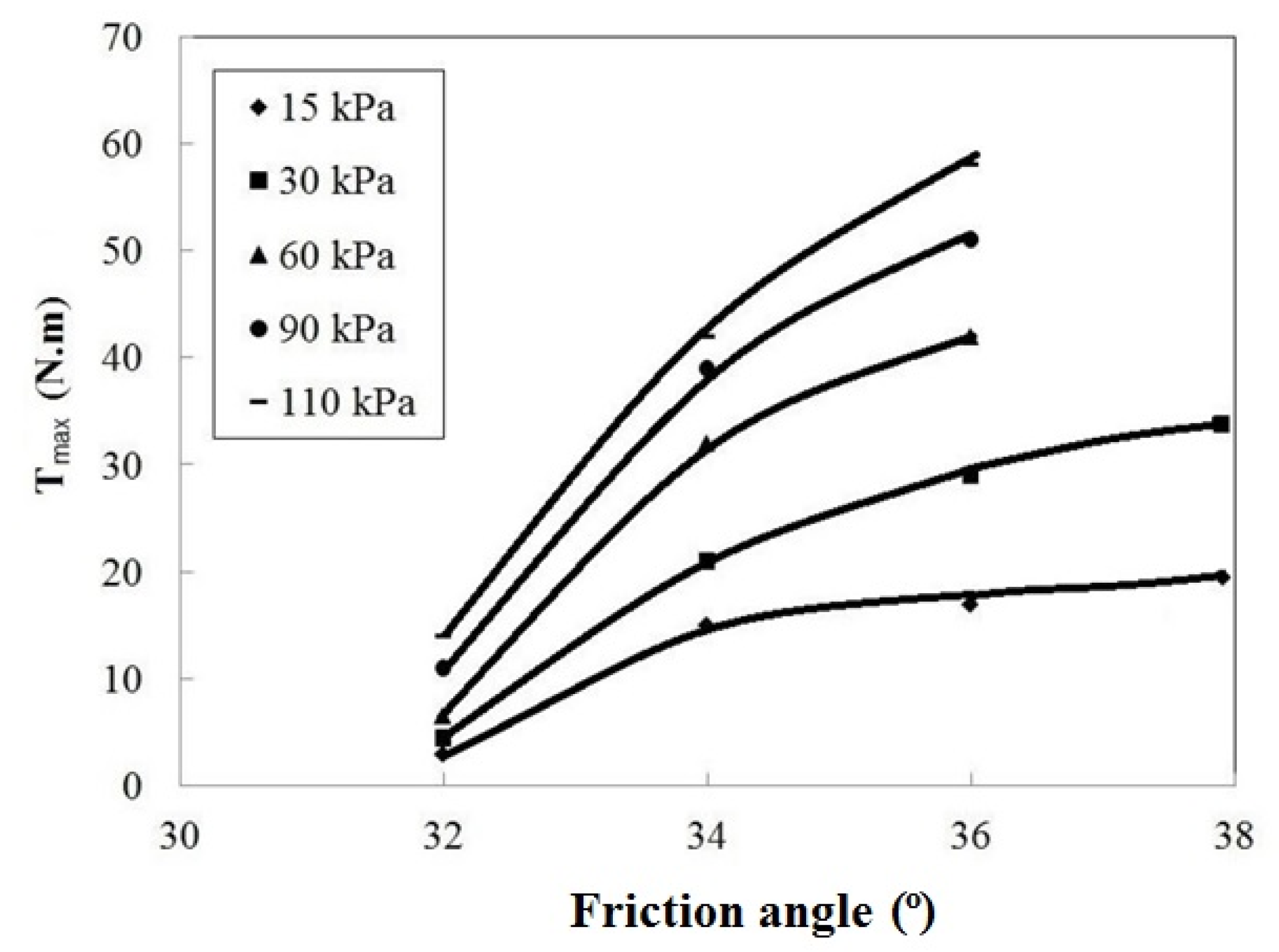
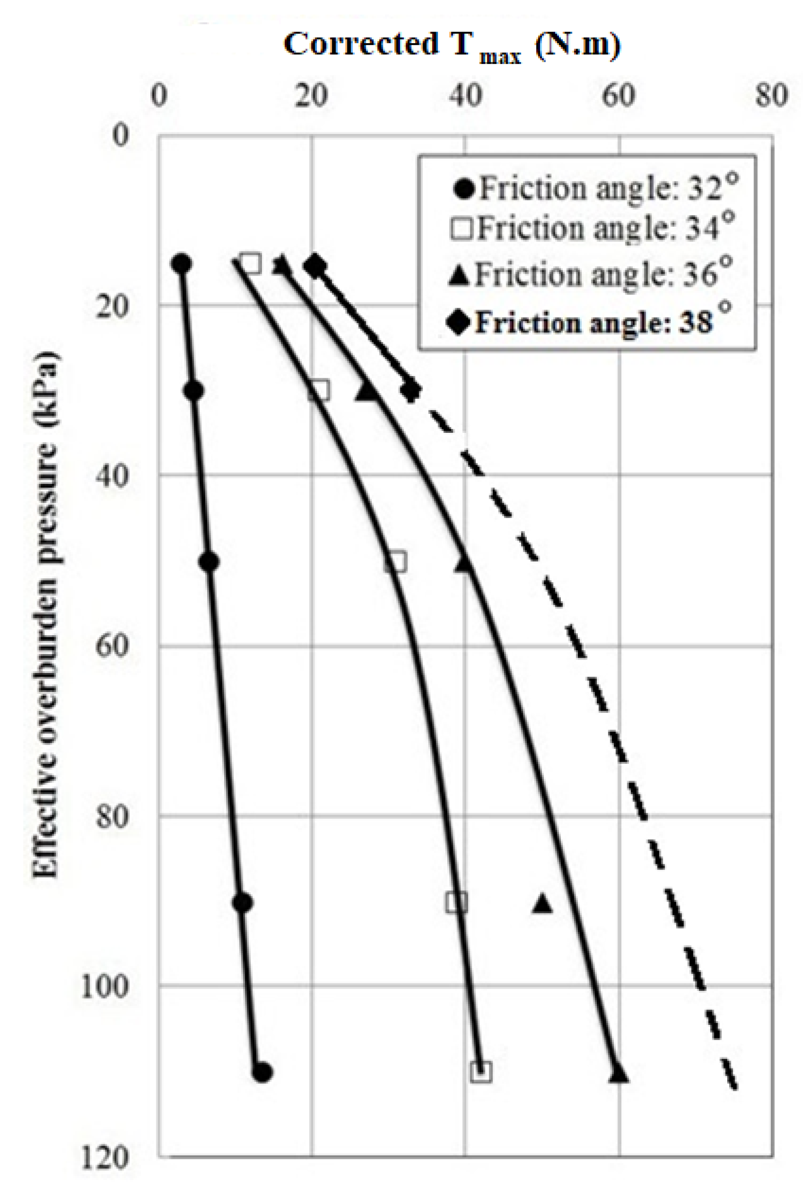
The obtained relationship presented in
Figure 10 can be transformed into a chart that can estimate the friction angle of the soil based on the measured torque in the SDS test.
Figure 11 shows the relationship between the torque, effective overburden pressure, and peak friction angle derived from the FE analyses. Due to the complexity and high computation cost, only two cases of overburden pressures of 15 and 30 kPa, respectively, at a friction angle of 38° were analysed. The dashed line in the figure represents extrapolation based on the observed trend. It can be seen that for a specific peak friction angle, the maximum torque increases as the overburden pressure increases, as expected in sandy soil with a drained behavior. This change is more significant for denser sands that have a higher peak friction angle. Moreover, for a constant overburden pressure, the difference in torque between peak friction angles of 32° and 34° is more significant than that between 34° and 36°. This is due to the assumption of a constant value of 33° for the critical state friction angle (i.e.,
) and the assignment of a dilation angle of 1° and 3° for the cases with friction angles of 34° and 36°, respectively. These assumptions imply that the behaviour of the soil with a friction angle of 32° is contractive, while soils with friction angles of 34° and 36° have dilative behaviour. When the drilling tool moves into a dilative soil under a specific confining pressure that prevents the soil from expanding, it needs more torque to move the soil away when compared to that when moving into the soil with a contractive behaviour. It should be noted that, as the whole soil domain is not simulated in the FE model, the effect of rod friction is not included in the analysis to obtain
. Therefore, the value of
obtained from the FE model is equivalent to the corrected torque of the SDS test.
The proposed chart can be used for predicting the angle of internal friction of soil using the SDS results. Caution should be exercised for shallow deposits, as the assumed elastic modulus is based on effective overburden pressure, and soils at shallower depth may be dense due to compaction and applied dynamic load on the ground surface, such as moving vehicles.
5.6. Model Evaluation
To verify whether the model can predict the friction angle of the soil with sufficient accuracy, the results of the SDS tests and laboratory element tests on samples taken at five different sites are compared to the results of the numerical modelling. For each test site described in
Table 3, the peak friction angles of the samples taken from specific depths were measured in the laboratory with consolidated drained triaxial tests [
11]. To use the chart shown in
Figure 11, the corrected
from the SDS tests, and the effective vertical stress (for the depth considered) are used to estimate the corresponding friction angle. The laboratory-derived friction angles, as well as the predicted values from the numerical model and summarised in a chart form, are presented in
Table 3. From the summary table, the proposed chart could estimate the peak friction angle with a high degree of accuracy.
It should be noted that there were several assumptions and limitations in both the modelling and experimental studies. Some of the model input parameters were assumed or estimated from empirical relationships, such as the coefficient of interface friction between the soil and the screw point, the value of Young’s modulus derived from an empirical relationship (Equation (10)), and the use of a simple constitutive model for the soil. For the experimental work, there were also uncertainties in the results of the laboratory tests conducted on reconstituted samples and the preparation of samples based on the estimated relative density from CPT. Considering these factors, the FE model predicted and correlated reasonably well with the laboratory results.
However, the results could be further improved with the use of more sophisticated constitutive models that can take into account other factors, such as the nonlinear behaviour of the soil, different stiffnesses for loading and unloading, and the dependency of soil stiffness on the stress/strain rate. Moreover, a more accurate estimation of the coefficient of interface friction is recommended, which can be obtained from laboratory tests. It is worth noting that one of the drawbacks of CEL analyses is the long computational time. The average computational time for simulation of the drilling process in this study was 36 h on a normal computer with a Core i5 processor.


