Article

From Crops to Kilowatts: An Empirical Study on Farmland Conversion to Solar Photovoltaic Systems in Kushida River Basin, Japan

1
Graduate School of Design, Kyushu University, Fukuoka 815-8540, Japan
2
Faculty of Design, Kyushu University, Fukuoka 815-8540, Japan
*
Author to whom correspondence should be addressed.
Geographies 2024, 4(2), 216-230; https://doi.org/10.3390/geographies4020014
Submission received: 1 February 2024 / Revised: 11 March 2024 / Accepted: 18 March 2024 / Published: 25 March 2024

Abstract

:
In Japan, rural areas are grappling with population decline and aging, leading to a shortage of labor for farmland maintenance. This has resulted in the abandonment of farmland or its conversion for solar photovoltaic (PV) use. However, this unplanned conversion raises concerns about agricultural productivity decline, landscape degradation, biodiversity loss, water resource maintenance, and disaster prevention. This study focuses on the Kushida watershed, examining (1) accurate farmland classification using remote sensing data, (2) the geographical distribution of farmland converted to PV systems from 2016 to 2021 and concentrated along the river, especially on north-facing slopes, (3) the highest conversion rates in wheat fields, followed by legume fields, tea fields, and paddy fields, and (4) no clear correlation between farmland conversions and changes in the number of farmers, but associations with farmland geography and solar radiation levels. These findings contribute to a nuanced understanding of sustainable rural development in Japan, emphasizing the importance of considering geographical factors in the conversion of farmland to PV.

1. Introduction

The rise in abandoned farmland and the expansion of construction areas pose both challenges and opportunities for land use in suburban and rural regions [1,2,3]. In Japan, a shortage of land managers has led to more farmers converting parts of their farmland into solar photovoltaic (PV) systems to generate additional income [4,5]. The fusion of agriculture and PV technology holds significant potential for reducing global reliance on fossil fuels and lowering CO2 emissions [6,7]. PV farms not only contribute to energy production but also bring social benefits, including food supplies and regional economic development [8,9]. The Japanese government aims for regional decarbonization by 2050, targeting a 46% reduction in greenhouse gas emissions from 2013 levels by 2030 [10]. The government actively encourages PV system implementation on unused rural land as part of this initiative.
Although PV systems are advancing at a fast pace, there is limited research available on the impact and consequence of the conversion of farmlands into PV systems on the surrounding environment. Mountainous environments are more sensitive than urban areas, and the construction of PV systems can have significant impacts on soil and climate, potentially affecting the surrounding or regional ecosystem patterns. Studies conducted by Adeh et al. [11] have shown that PV construction in mountainous environments can have adverse effects on soil and climate. Additionally, research by Jiang et al. (2022), Zhang et al. (2023), and Zheng et al. (2023) [12,13,14] demonstrated that PV construction can impact the ecosystem patterns in surrounding or regional areas. The transformation of agricultural land into PV systems, as a complete land use change, is believed to have significant impacts on the surrounding environment and particularly on crop growth [11]. In watershed areas, farmland not only contributes significantly to the landscape and food supply but also has the potential to address flooding hazards [12,13], indirectly leading to an increased risk of flooding. Additionally, due to the strong relationship between farmland and biodiversity [14,15], converting large areas of farmland threatens local ecological balance.
Despite these concerns, research on the actual conversion of farmland into PV systems, considering both human and geographical factors, is limited. In the central region of Japan, home to the largest tea plantations and rice fields, farmland is a vital part of the local landscape. However, depopulation in suburban and rural areas is accelerating farmland abandonment [16,17]. Despite strict regulations on land use conversion in Japan [18], many landowners have opted to convert farmland into PV systems, prompting environmental concerns from the government and citizens [1,19]. In Mie Prefecture, the ordinance related to the introduction of PV systems was revised in April 2022, establishing guidelines and regulations for PV system installation in productive green spaces. However, to avoid stricter regulations, many farmers converted their farmlands into PV systems before the ordinance was enacted in 2022, resulting in a series of environmental issues. Given that crop growth depends on a suitable environment, any changes in the surroundings may lead to decreased crop yield and quality [20,21,22]. Therefore, a deeper understanding of farmland conversion patterns into PV is crucial to effectively address these concerns.
In this study, our focus was on exploring the geographic causes behind the conversion of various farmland types to photovoltaic (PV) systems. Employing remote sensing data and a machine learning model, we categorized farmland based on crop types. Subsequently, we conducted a spatial analysis on four types of farmlands to examine the patterns of land conversion into PV systems, taking into account geographical conditions, population changes, and management costs. What distinguishes our study from existing research is our specific emphasis on farmland conversion to PV systems and the integrated analysis of both social factors and geographic characteristics. Through this approach, we acquired insights into farmland geographical features and investigated the relationships between land conversion and both geo and socio-economic factors. The study yielded the following key findings:
We confirmed the effectiveness of farmland classification using NDVI and MNDWI in the watershed area, enabling the accurate categorization of crop types based on growth status and the presence of water bodies.
Spatial information was acquired to comprehend the geographic conditions influencing the conversion of farmland into PV systems. This involved analyzing the position and distribution patterns of converted land and examining their correlation with the surrounding topography and water bodies, thereby identifying factors influencing PV system sizing.
By comprehensively investigating both geographic and social factors, we identified patterns of farmland conversion into PV systems based on crop types. Specifically, analyzing the relationships between land conversion, geographic factors, and social factors revealed distinct conversion patterns based on crop type.

2. Materials and Methods

2.1. Site Description and Data Collection

This research is focused on the Kushida River basin in Mie Prefecture, located in the central part of Japan (Figure 1). It encompasses the following three areas: Matsusaka City, Taki Town, and Meiwa Town. With a total area of 767.62 km2 and a population of approximately 200,000 (2015), it is a typical agricultural city, where forests and farmland account for about 82% of the total area. However, due to depopulation, a significant portion of the farmland in this region has been converted into PV systems. This raises concerns not only about increased flood risks in the watershed but also about significant impacts on the surrounding ecosystems. According to the official investigation results from the Japanese government (Table 1), the Kushida River basin, where the study area is located, is facing a severe decline in population, concurrent with a reduction in the agricultural land area. Over the decade from 2010 to 2020, the population in the area decreased by 10.1%, while the agricultural land area decreased by 6.3%. The agricultural economic output also declined by 7.3%, indicating the decline of agriculture, which is the pillar industry of this region.
The data sources for this study included satellite images (Sentinel-2), official government databases, and on-site surveys. Remote sensing has been widely applied in land use and agricultural research [23,24,25]. In this study, the location and type of farmland are considered to be factors that influence the rate of conversion to land for PV. Additionally, the crop type also affects the location conditions and labor required for management. Therefore, conversion for solar panel use was observed and analyzed separately for each crop type, aiming to examine the specific impacts of geographical factors on different crops. Given the presence of numerous small-scale agricultural plots within the study area, Sentinel-2 images from the European Space Agency (ESA) were used for a more accurate classification of land types. The farmland polygons and farming community data were downloaded from the Ministry of Agriculture, Forestry, and Fisheries of Japan (MAFF) for 2016 and 2021, respectively. Geographical features such as digital elevation models (DEMs), road networks, river data, and aerial photographs for PA extraction were acquired from public data provided by the Geospatial Information Authority of Japan.

2.2. Model Structures and Simulation Methods

The workflow used in this study is illustrated in Figure 2. Firstly, the monthly NDVI and MNDWI for the study area from 2016 to 2017 using Sentinel-2 data was calculated. Then, a machine learning model called Random Forest (RF) was implemented to classify the farmland into the following four types: paddy fields (PFs), wheat fields (WFs), tea fields (TFs), and bean fields (BFs). The positions of the PV systems in the study area were identified using a combination of ArcGIS Pro’s deep learning module and manual corrections based on aerial photographs taken in 2021. Based on these data, the number and locations of farmland units converted into solar panels were determined from 2016 to 2021. Finally, combining social factors (population changes) and geographic factors is conducted to derive conversion patterns for each crop type.

2.2.1. Classification of Farmland with Sentinel-2 Data

The farmland locations were obtained from the MAFF and imported into ArcGIS as polygons. Based on the on-site interviews (25 local farmers in 2021), the farmland in this area was classified into the following four categories: “Paddy Fields (PFs)”, “Wheat Fields (WFs)”, “Tea Fields (TFs)”, and “Bean Fields (BFs)”.
The distinguishing feature of PFs is the presence of water bodies during the irrigation period. Therefore, the modified normalized difference water index (MNDWI) [26,27] was used to differentiate PFs from other types of farmland. The calculation formula (1) for the MNDWI is an improvement of the NDWI calculation formula proposed by XU (2007) [28] based on the McFeeters (1996) [29]:
M N D W I = G S W I R / G S W I R
where G represents the green band value, and SWIR represents the Short-Wave Infrared Radiometer band value. MNDWI is an index for water area determination; it is performed for each field by overlaying the field plot data on the MNDWI image that is binarized (threshold values are automatically determined by Otsu’s method). Establishing a threshold based on MNDWI allows the differentiation of paddy fields (PFs) from other farmlands. For the period from February to June 2017, corresponding to the PF irrigation season, we computed MNDWI temporal change images in the study area. The statistical analysis led to the setting of a threshold at −0.022. Subsequently, using the MAFF’s farmland location data, we extracted regions with MNDWI values surpassing the threshold (indicating water) and calculated the areas and counts of PFs (Figure 3).
As various crops exhibit distinct growth cycles, their patterns observed through remote sensing data differ. To distinguish the remaining three crop types, variations in the normalized difference vegetation index (NDVI) were considered. NDVI, widely accepted as a vegetation indicator, estimates vegetation density by computing the difference in reflectance between visible and near-infrared light [30] (Equation (2)). NDVI finds extensive application in vegetation monitoring and agriculture for tracking changes and assessing vegetation health [31,32,33]:
N D V I = N I R R / N I R + R
where NIR represents near-infrared reflectance and R represents red reflectance.
The monthly NDVI values from November 2016 to October 2017 using Sentinel-2 images were calculated using Equation 2. However, NDVI values for January, July, and October were not calculated due to cloud cover. Utilizing the 9-month NDVI as an independent variable, the Random Forest (RF) model was applied to classify farmland into the following three types: wheat fields (WF), tea fields (TF), and bean fields (BF). During field surveys, 154 TF, 206 WF, and 150 BF samples were manually labeled. The labeled samples were then used to train and test the model with corresponding NDVI values (Figure 4). RF is a machine learning method widely used in landscape analysis [34,35,36,37] due to its high accuracy and ability to handle small sample sizes [38].
The RF model is an ensemble of decision trees based on the bootstrap sampling of the training data, and the final prediction is obtained by averaging the predictions of all the trees [39]. The calibration of the RF model involves the following three parameters [40]: the number of trees (n_tree), the number of covariates selected at each split (m_try), and the size of the terminal nodes (node_size). In this study, after multiple trials and adjustments, we set n_tree = 300, node_size = 6, and m_try = 3. Among the 510 samples, 70% were used as training samples, and 30% were used as test samples.

2.2.2. Locating the Agricultural Land Converted into PV Systems (2016 to 2021)

To identify the farmland converted to PV systems between 2016 and 2021, the 2021 aerial photographs were analyzed using the DeepLab model. It is a deep learning module in ArcGIS Pro [41,42]. DeepLab is an image analysis model based on Fully Convolutional Neural Networks (FCNs) that can extract specific objects from images. It is widely used in land use and environmental green space fields [43,44]. This tool extracted the polygon data of all PV systems in the study area from the 2021 aerial photographs and conducted the manual verification and correction of the results. Then, ArcGIS was used to juxtapose the PV system polygons with the 2016 farmland data. This enabled us to determine the number and locations of farmland areas that were converted to solar panels for each crop type from 2016 to 2021 (Figure 5). It is important to note that the area of the PV system might partially match the original farmland area. For this study, if the PV system utilizes more than 50% of its area, it is considered to be converted.

2.2.3. Analysis of Motives for Farmland Diversion

To study what causes farmland to change, it is important to look at both geographical and human elements. This study explored the human factors influencing farmland conversion, focusing on how the number of farmers in each village changes. Data from the Japanese government (E-stat) on the number of farmers in each village was extracted and imported to ArcGIS as shape layers. The following formula was used to calculate the personal farming rate (PFR) from 2016 to 2021. This rate shows how the number of individual farmers has changed. We also calculated the farmland conversion rate (FCR) for each village, showing how much farmland has turned into PV systems. By looking at these two rates, we could understand how the change in the number of farmers and the conversion of farmland are related.
P F R j = P F N j 2020 P F N j 2015 P F N j 2015 × 100 %
F C R j = C L j F L j × 100 %
where PFRj represents the change rate in the farmer population in area j. PFNj represents the number of farmers in area j, FCRj represents the farmland conversion rate in region j, CLj denotes the number of converted farmlands in region j, and FLj represents the total farmland area in region j in 2016. We used multiple regression to see how changes in farmer numbers and six geographical factors for (1) slope direction, (2) slope angle, (3) elevation (DEM), (4) openness, (5) distance to water (WD), (6) distance to roads (RD) are affecting farmland conversion. Openness expresses the dominance (positive) or enclosure (negative) of a landscape location. See Yokoyama et al. (2002) 0 for a precise definition. Openness has been related to how wide a landscape can be viewed from any position.
Additionally, we performed a separate analysis for different farmland types to see the geographical traits of converted lands. We used one-way ANOVA to check if there was a significant difference in geographical features among various farmlands and converted lands. One-way ANOVA is a filter to select the relevant factor and is used in most landscape studies [45,46,47,48]. One-way ANOVA has proven its effectiveness in solving the problem of high dimensionality in the feature space [49,50].
Some studies have shown that solar radiation profiles greatly affect the reliability of PV system sizing [20,51]. To confirm whether these findings also apply to the river basin area, we used the solar radiation analysis tool in ArcGIS to calculate and compare the solar radiation levels in the farmland areas and the regions converted into PV systems.

3. Results

3.1. Farmland Classification Model Results

To determine the accuracy of the farmland classification model, we used the confusion matrix to validate the results. The accuracy value and confusion matrix were employed as criteria for determining the accuracy of the RF model. The accuracy value of a model is a measure that describes its overall accuracy and was determined in this study using the following equation:
A c c u r a c y = T W F + T B F + T T F / S n
where TWF, TBF, and TTF represent the number of WF, BF, and TF instances accurately predicted by the model based on the test samples, while Sn represents the total number of test samples. The accuracy value of the model constructed in this step reached 0.91, suggesting the effectiveness of the model. The confusion matrix (Table 2) reveals the prediction accuracy for each land type. Among them, TF extraction demonstrated the highest precision at 93%. This can be attributed to the fast growth cycle of TFs. However, our model did not include other farmlands like fruit or vegetable farms or unused lands, which might have caused some errors.
Based on the classification results, it can be observed that PFs have the highest quantity and occupy the largest area within the study zone (Figure 6a). PFs and WFs exhibit similar distribution patterns, primarily located in low-lying flatlands and suburban areas. TFs, on the other hand, are lower in numbers and are mainly situated in high-altitude regions such as mountainous areas. The BFs are distributed in multiple locations and are relatively more dispersed in their distribution, though they are concentrated primarily near rivers (Figure 6b).

3.2. Conversion of Farmland into PV Systems

According to the calculations, a total of 1806 new PVs were constructed in the study area between 2016 and 2021, with a total area of 394.8 ha. Regarding farmland conversion, of approximately 106,000 locations, 1052 sites were converted to PV systems, accounting for 0.98% of the total, with an area of 77.93 ha. Considering that this change occurred within a span of just five years, it is a noteworthy trend. In terms of land types, WFs have the highest number of conversion instances, with 20 hectares (0.93%) out of a total of 1019 hectares being converted into PV systems. On the other hand, TFs and PFs have conversion rates of only 0.47% and 0.54%, respectively (Table 3).
When analyzing the number of converted fields to solar panels, both suburban areas and mountainous areas exhibited a high density (Figure 7a). However, when considering the converted area, it was found that this high density was concentrated only in the suburban areas.

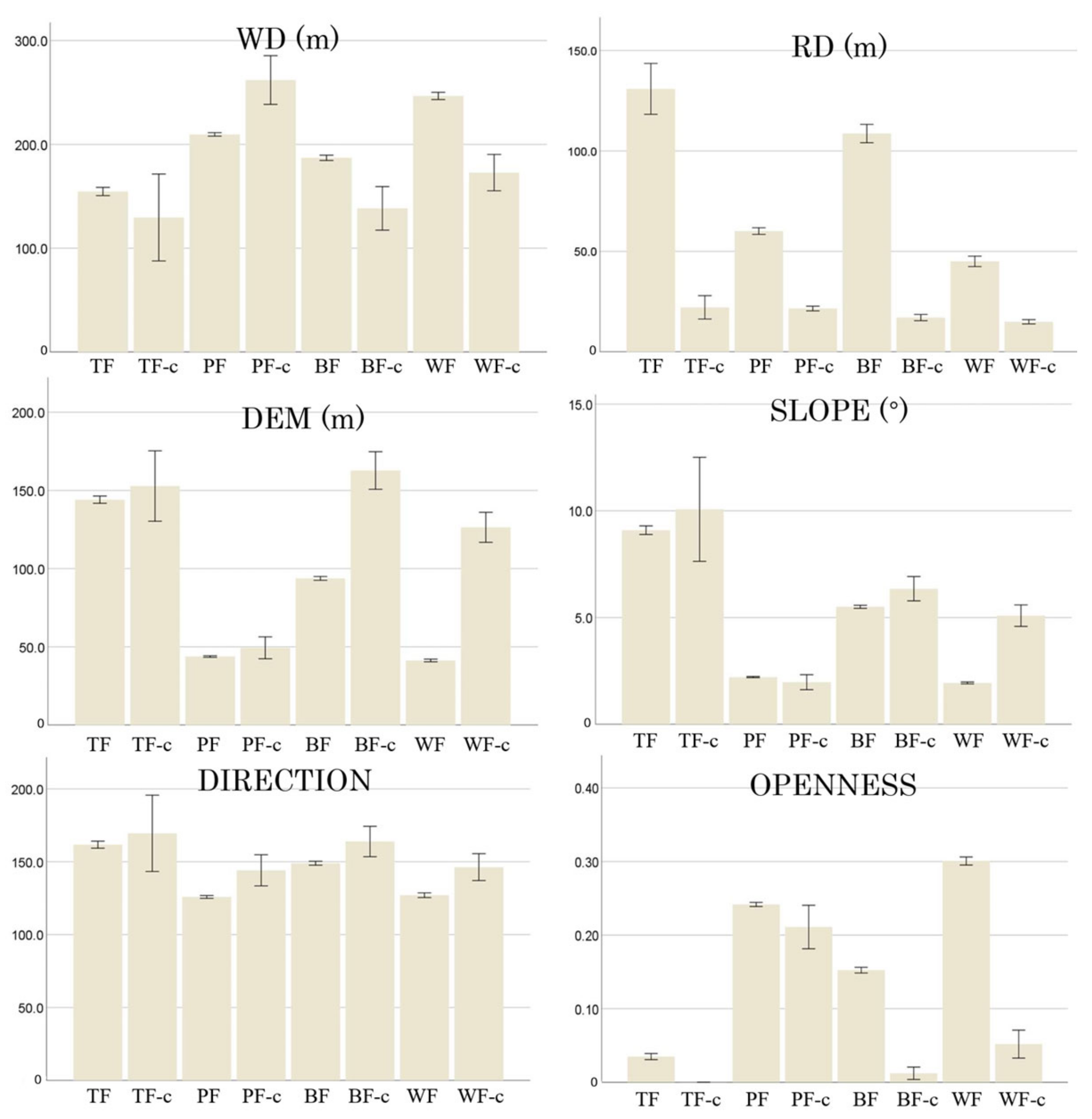
3.3. Analysis of GEO-Motives for Conversion of Farmland

The ANOVA showed significant (at 0.01 level) geographical differences between converted land and all farmlands Table 4).
These significant differences suggest that geographical features are key in farmland conversion. To understand their specific impact (positive or negative), we compared the average values of these features for both converted and unconverted farmlands. As shown in Figure 8 and Table 5, average values were calculated for farmland and converted land based on various geographical features, as follows:
(1)
Water source distance (WD): converted TFs, BFs, and WFs are closer to the average distance to water sources than PF, which is 20% further.
(2)
Road distance (RD): converted lands are generally closer to roads, usually less than 25 m away.
(3)
Elevation (DEM): both BF and WF conversions seem influenced by elevation, with WF conversions more common in higher-elevation areas.
(4)
Slope: WFs show a relationship with slopes, indicating more conversions in steeper areas.
(5)
Slope direction (DIRECTION): there is no clear trend, but converted lands often face southeast.
(6)
Openness (OPEN): this impacts BF, WF, and TF conversions, with converted lands typically having lower average openness values, affecting factors like sunlight duration.
By analyzing the relationships between farmland conversion and geographical factors, we identified the positive and negative factors influencing the conversion of each type of farmland (Table 6). “PST” represents the fact that larger values of the geographic factor have a positive impact on the farmland in terms of its conversion to PV systems. “NGT” representing the larger values have a negative impact on farmland in the conversion to a PV. “/” means that the corresponding factor has no effect on the farm’s conversion.
Then, we calculated the annual solar radiation for all types of farmland and conversion sites (Table 7). The results show that the annual total solar radiation that the conversion sites receive is 2,265,092 W/m2, surpassing both the average for the entire Kushida River basin (1,916,778 W/m2) and the average for all types of farmland (1,961,580 W/m2). Furthermore, the conversion sites even exceed the average solar radiation of existing PV systems (1,959,251 W/m2) by 15%. This suggests that solar radiation is an important factor in the conversion of farmland into PV systems.

3.4. Social Factors Related to the Conversion of Farmland

In our study, we found that 68 villages (a total of 345 villages) experienced farmland conversion between 2016 and 2021, with FCR ranging from 0.1% to 38% (Figure 9a). During these five years, the PFR in the study area decreased by 29.1% overall, with 224 villages experiencing a PFR change, with changes in the villages ranging from a decrease of 83% to an increase of 11% (Figure 9b).
The results of our multiple regression analysis (Table 8) show that the significance probability is less than 0.01, indicating the significance of the model. The R-squared value is 0.244, indicating that the variables in this model explain 24% of the variation in the FCR. Moreover, the significance of each variable could be determined based on the significance probability (P), and we found that the four variables in this model could be studied using the beta value, where the greater the value of beta is, the greater its effect on the dependent variable is. The slope direction, slope angle, elevation (DEM), and distance to roads (RDs) are significant explanatory variables (p < 0.05, beta >0.1 or <−0.1). However, no correlation was found between the personal farming rate (PFR) and the farmland conversion rate (FCR).

4. Discussion

This study classified farmland based on crop type and examined the tendency of each type to be converted into PV systems.

4.1. Current Land Use after Farmland Conversion

In this study, about 78 ha of the farmland was converted into PV systems within 5 years. Most of the farmland conversions were spread out near the river. Regarding the conversion tendencies of different types of farmlands, the conversion rate was highest for WFs (1.7%) and lowest for TFs (0.66%). PFs and TFs, which are considered the main local crops, have the lowest rates of conversion into PV systems.

4.2. Relationship between Farmland Conversion and GEO-Motives

Furthermore, we found that the conversion of each type of farmland is influenced by its geo-characteristics and cultivation environment. In general, all types of farmlands closer to roads tend to have higher chances of conversion. This could be attributed to the exhaust and dust from vehicles on roads, which may negatively affect crop quality, encouraging people to convert their own farmland; also, being close to the road makes maintenance and repair more convenient. From the tendency to convert each type of farmland, we obtained the following conclusions. (1) The conversion of WFs is closely related to each geo-characteristic except the direction. This is likely due to the higher labor demand for WFs compared to other types of farmlands, making it economically unfeasible to allocate labor and income in areas with harsh conditions, such as high-elevation areas in mountainous regions. (2) Since BFs and WFs are both dryland crops, their growing conditions are not very different. Therefore, the geo-characteristics of conversion land are almost the same for both except for the slope angle. This is because there are quite a few terraces in the local BF, and the significance of terraces in mitigating the influence of slope angle on crop cultivation has far-reaching implications for sustainable agriculture and land use management. Terraces, as a cultural and environmental heritage of the local landscape, are constrained and protected in terms of land use 0. Therefore, the inclination of the land does not affect the cultivation of BF. Similarly, TFs and PFs are not affected by slopes for the same reason. (3) PFs tend to be more easily converted when they are situated further away from waterways, which can be attributed to their unique cultivation environments and the need for water resources in PFs. Our on-site interviews with PF farmers revealed that irrigation-related tasks, such as pump installation and water channel maintenance, incurred significant management costs, making natural gravity-fed irrigation the most convenient method. Thus, the tendency of PFs to be converted aligns with their distance from water sources. Additionally, there was almost no correlation found between the slope direction of farmland and its conversion into land for PV systems. (4) The conversion of TFs as a high-value crop is influenced by RD while also correlated with openness.
When considering the conversion of all types of farmlands, it was observed that farmland conversion primarily occurred in localized settlements along rivers. In particular, only the northern side of the river was utilized for conversion in the downstream and middle reaches (where elevation is lower than 200 m). When combined with the analysis of solar radiation, it could be inferred that the location of farmland along rivers and in the middle and lower reaches provides longer exposure to sunlight, maximizing the efficiency of PV system utilization.

4.3. Relationship between Farmland Conversion and Social Detective

In this study, when we analyzed a village unit level, no direct relationship was found between the conversion rate of farmland and the increase or decrease in the number of farmers. It is possible that individual farmers own multiple plots of land and do not convert all of them. Factors such as the aging of agricultural operators and changes in the surrounding environment should also be considered. Additionally, the number of farmland plots owned by a single farmer varies, and future research should also take these factors into account.

4.4. Relative Research about PV Location Character

From a macro-planning perspective, solar energy utilization significantly shows characteristics of resource dependence and policy-driven aspects, with varying driving factors across different study scales and regions. Studies based on urban and mixed areas suggest that PV site selection is often determined by investment costs and economic benefits [52,53,54]. Our research indicates that in watershed areas, geographical factors like elevation, slope, and solar radiation are key drivers for PV site selection, while social factors like population change have little impact. This aligns with the findings by SUN [55] in plains and macro areas. In some studies on PV site selection in mountainous areas [56], proximity to roads is considered a positive factor, which is consistent with our findings that farmlands converted to PV are mostly near roads.

4.5. The Potential Impacts on the Environment

The conversion of farmland to PV may have significant effects on the surrounding environment. Changing land use from farmland to PV implies a loss of permeable layers and an increase in impermeable surfaces. Such changes undoubtedly affect the local ecological environment. Some studies suggest that constructing PV in desert areas increases the soil moisture content, but in watershed regions, this change may exacerbate the risk of flooding. Although, there may be alterations in the infiltration and retention of water within the soil. This could potentially exacerbate drought conditions by reducing soil moisture availability for agricultural activities and natural vegetation. With less vegetation to intercept rainfall and facilitate evapotranspiration, there could be increased surface runoff and reduced groundwater recharge. This disruption to the natural water balance might contribute to a decline in water availability during dry periods, exacerbating drought conditions in the watershed.
Additionally, the presence of large arrays of solar panels can create localized warming effects, known as the “heat island” effect, due to the absorption and re-radiation of solar energy. These elevated temperatures can further exacerbate drought conditions by increasing evaporation rates and intensifying water stress on vegetation and soil moisture.

4.6. Limitations and Prospects

Our proposed methodological framework fills a gap in identifying the spatial distribution of farmland conversion to PV in watershed regions and is a strong reference for modeling farmland conversion and land use changes. This framework can also be applied to other regions or countries, aiding in more accurately identifying suitable areas for PV and site selection criteria. However, this work has limitations, such as a limited number of samples involved, which should be increased for macro studies. Additionally, the accuracy of the model and the limited number of dependent variables should be expanded in future research to consider more detailed influencing factors.

5. Conclusions

This study conducted a classification survey of farmland within a watershed area, revealing that the factors influencing the conversion of these lands to PV systems vary based on the type of agricultural land. The results indicate that, over a span of five years, a total of 77.93 ha (0.64%) of agricultural land was converted to PV systems, with most of the locations concentrated near streams. While the PFs in the study area were converted the most overall, in terms of the percentage, WFs were converted close to one percent of the area. Conversion factors were found to be influenced by geographical conditions specific to each agricultural land type, with the distance to roads and annual solar radiation directly affecting the conversion of almost all types of agricultural land. Furthermore, the impact of population change was almost negligible in relation to the conversion to PV. By combining a Random Forest (RF) model with the one-way analysis of variance (ANOVA) method, this study analyzed changes in different types of agricultural land, revealing various driving factors and suggesting the complexity of causal relationships controlling watershed land use change. Through the comparative analysis of influencing factors across diverse topographic zones, we shed light on the nuanced dynamics of land use change in varied geographical contexts. The findings of this study hold relevance beyond the specific watershed examined, providing valuable insights into the broader mechanisms driving agricultural land conversion. Since most of the data used in the study are from public websites, we believe that the methodology used in the study can still be applied to non-specific areas on a global scale. Such methods are instrumental in guiding future research and policymaking endeavors aimed at sustainable land management and renewable energy integration.

Author Contributions

Conceptualization, Z.X. and C.T.; methodology, Z.X.; software, Z.X.; validation, Z.X. and C.T.; formal analysis, Z.X.; investigation, Z.X. and S.M.A.U.; resources, C.T.; data curation, Z.X. and C.T.; writing—original draft preparation, Z.X. and C.T.; writing—review and editing, S.M.A.U.; visualization, Z.X.; supervision, C.T. and S.M.A.U.; project administration, Taktori; funding acquisition, C.T. All authors have read and agreed to the published version of the manuscript.

Funding

This work was supported by the Japan Science and Technology Agency SPRING Project (grant number JPMJSP2136), the Japan Science and Technology Agency RISTEX Project (grant number JPMJRX20B3), and also supported by JSPS KAKENHI Grant-in-Aid for Scientific Research (B) (grant number 23H01584).

Data Availability Statement

Raw data used in this research were generated at USGS, ESA and MAFF. Derived data supporting the findings of this study are available from the corresponding author Chika Takatori on request.

Conflicts of Interest

The authors declare no competing interests.

References

  1. Kim, J.Y.; Koide, D.; Ishihama, F.; Kadoya, T.; Nishihiro, J. Current Site Planning of Medium to Large Solar Power Systems Accelerates the Loss of the Remaining Semi-Natural and Agricultural Habitats. Sci. Total Environ. 2021, 779, 146475. [Google Scholar] [CrossRef]
  2. Yang, Y.; Hobbie, S.E.; Hernandez, R.R.; Fargione, J.; Grodsky, S.M.; Tilman, D.; Zhu, Y.-G.; Luo, Y.; Smith, T.M.; Jungers, J.M.; et al. Restoring Abandoned Farmland to Mitigate Climate Change on a Full Earth. One Earth 2020, 3, 176–186. [Google Scholar] [CrossRef]
  3. Zhou, Y.; Chen, T.; Feng, Z.; Wu, K. Identifying the Contradiction between the Cultivated Land Fragmentation and the Construction Land Expansion from the Perspective of Urban-Rural Differences. Ecol. Inform. 2022, 71, 101826. [Google Scholar] [CrossRef]
  4. Goto, S.; Angchaisuksiri, P.; Bassand, J.-P.; Camm, A.J.; Dominguez, H.; Illingworth, L.; Gibbs, H.; Goldhaber, S.Z.; Goto, S.; Jing, Z.-C.; et al. Management and 1-Year Outcomes of Patients with Newly Diagnosed Atrial Fibrillation and Chronic Kidney Disease: Results from the Prospective GARFIELD-AF Registry. J. Am. Heart Assoc. 2019, 8, e010510. [Google Scholar] [CrossRef]
  5. Nozu, T. Analysis on Farmers’ Willingness of Implement to Combinations of Solar Photovoltaic and Food Crops. J. Rural. Plan. Assoc. 2018, 37, 304–311. [Google Scholar] [CrossRef]
  6. Pascaris, A.S.; Schelly, C.; Burnham, L.; Pearce, J.M. Integrating Solar Energy with Agriculture: Industry Perspectives on the Market, Community, and Socio-Political Dimensions of Agrivoltaics. Energy Res. Soc. Sci. 2021, 75, 102023. [Google Scholar] [CrossRef]
  7. Qerimi, D.; Dimitrieska, C.; Vasilevska, S.; Alimehaj, A. Modeling of the Solar Thermal Energy Use in Urban Areas. Civ. Eng. J. 2020, 6, 1349–1367. [Google Scholar] [CrossRef]
  8. Agostini, A.; Colauzzi, M.; Amaducci, S. Innovative Agrivoltaic Systems to Produce Sustainable Energy: An Economic and Environmental Assessment. Appl. Energy 2021, 281, 116102. [Google Scholar] [CrossRef]
  9. Kumpanalaisatit, M.; Setthapun, W.; Sintuya, H.; Pattiya, A.; Jansri, S.N. Current Status of Agrivoltaic Systems and Their Benefits to Energy, Food, Environment, Economy, and Society. Sustain. Prod. Consum. 2022, 33, 952–963. [Google Scholar] [CrossRef]
  10. Carbon Neutrality | Global Issues-JapanGov. Available online: https://www.japan.go.jp/global_issues/carbon_neutrality/ (accessed on 24 January 2024).
  11. Adeh, E.H.; Selker, J.S.; Higgins, C.W. Remarkable Agrivoltaic Influence on Soil Moisture, Micrometeorology and Water-Use Efficiency. PLoS ONE 2018, 13, e0203256. [Google Scholar] [CrossRef]
  12. Kenyon, W.; Hill, G.; Shannon, P. Scoping the Role of Agriculture in Sustainable Flood Management. Land Use Policy 2008, 25, 351–360. [Google Scholar] [CrossRef]
  13. Posthumus, H.; Hewett, C.J.M.; Morris, J.; Quinn, P.F. Agricultural Land Use and Flood Risk Management: Engaging with Stakeholders in North Yorkshire. Agric. Water Manag. 2008, 95, 787–798. [Google Scholar] [CrossRef]
  14. Kehoe, L.; Senf, C.; Meyer, C.; Gerstner, K.; Kreft, H.; Kuemmerle, T. Agriculture Rivals Biomes in Predicting Global Species Richness. Ecography 2017, 40, 1118–1128. [Google Scholar] [CrossRef]
  15. Wang, C.-J.; Wan, J.-Z.; Fajardo, J. Effects of Agricultural Lands on the Distribution Pattern of Genus Diversity for Neotropical Terrestrial Vertebrates. Ecol. Indic. 2021, 129, 107900. [Google Scholar] [CrossRef]
  16. Ajiki, K. Changes in the Structure of Industries and Reduction of Agriculture in Mountain Villages of Mie Prefecture, Japan since the 1990s. Jinbun Ronso Bull. Fac. Humanit. Law Econ. 2020, 37, 1–13. [Google Scholar]
  17. Yamada, S.; Okubo, S.; Kitagawa, Y.; Takeuchi, K. Restoration of Weed Communities in Abandoned Rice Paddy Fields in the Tama Hills, Central Japan. Agric. Ecosyst. Environ. 2007, 119, 88–102. [Google Scholar] [CrossRef]
  18. Kamigawara, K.; Yuichiro, M. Regulation on Location of Solar Photovoltaic Stations by Local Ordinances to Regulate Location of Renewable Energy Power Stations. Pap. Environ. Inf. Sci. 2020, 34, 323–328. [Google Scholar]
  19. Kazuki, K.; Kunihiko, M.; Masanori, S. Validity of Ordinances that Control Developments of Solar Panels on the ground for Location and Landscape Conservation. J. City Plan. Inst. Jpn. 2018, 53, 1313–1319. [Google Scholar] [CrossRef]
  20. Abdulkarim, H.T.; Sansom, C.L.; Patchigolla, K.; King, P. Statistical and Economic Analysis of Solar Radiation and Climatic Data for the Development of Solar PV System in Nigeria. Energy Rep. 2020, 6, 309–316. [Google Scholar] [CrossRef]
  21. Krishnan, P.; Ramakrishnan, B.; Reddy, K.R.; Reddy, V.R. Chapter Three—High-Temperature Effects on Rice Growth, Yield, and Grain Quality. In Advances in Agronomy; Sparks, D.L., Ed.; Academic Press: Cambridge, MA, USA, 2011; Volume 111, pp. 87–206. [Google Scholar]
  22. Song, Y.; Wang, C.; Linderholm, H.W.; Fu, Y.; Cai, W.; Xu, J.; Zhuang, L.; Wu, M.; Shi, Y.; Wang, G.; et al. The Negative Impact of Increasing Temperatures on Rice Yields in Southern China. Sci. Total Environ. 2022, 820, 153262. [Google Scholar] [CrossRef]
  23. Alcantara, C.; Kuemmerle, T.; Prishchepov, A.V.; Radeloff, V.C. Mapping Abandoned Agriculture with Multi-Temporal MODIS Satellite Data. Remote Sens. Environ. 2012, 124, 334–347. [Google Scholar] [CrossRef]
  24. Friedl, M.A.; Brodley, C.E. Decision Tree Classification of Land Cover from Remotely Sensed Data. Remote Sens. Environ. 1997, 61, 399–409. [Google Scholar] [CrossRef]
  25. Minghua, W.; Yueming, H.; Hongmei, W.; Guangsheng, L.; Liying, Y. Remote Sensing Extraction and Feature Analysis of Abandoned Farmland in Hilly and Mountainous areas: A Case Study of Xingning, Guangdong. Remote Sens. Appl. Soc. Environ. 2020, 20, 100403. [Google Scholar] [CrossRef]
  26. Anusha, B.N.; Babu, K.R.; Kumar, B.P.; Kumar, P.R.; Rajasekhar, M. Geospatial Approaches for Monitoring and Mapping of Water Resources in Semi-Arid Regions of Southern India. Environ. Chall. 2022, 8, 100569. [Google Scholar] [CrossRef]
  27. Gautam, V.K.; Gaurav, P.K.; Murugan, P.; Annadurai, M. Assessment of Surface Water Dynamicsin Bangalore Using WRI, NDWI, MNDWI, Supervised Classification and K-T Transformation. Aquat. Procedia 2015, 4, 739–746. [Google Scholar] [CrossRef]
  28. Xu, H. Modification of Normalised Difference Water Index (NDWI) to Enhance Open Water Features in Remotely Sensed Imagery. Int. J. Remote Sens. 2006, 27, 3025–3033. [Google Scholar] [CrossRef]
  29. Mcfeeters, S.K. The Use of the Normalized Difference Water Index (NDWI) in the Delineation of Open Water Features. Int. J. Remote Sens. 1996, 17, 1425–1432. [Google Scholar] [CrossRef]
  30. Townshend, J.R.G.; Justice, C.O. Analysis of the Dynamics of African Vegetation Using the Normalized Difference Vegetation Index. Int. J. Remote Sens. 1986, 7, 1435–1445. [Google Scholar] [CrossRef]
  31. M, S.K.; Jayagopal, P. Delineation of Field Boundary from Multispectral Satellite Images through U-Net Segmentation and Template Matching. Ecol. Inform. 2021, 64, 101370. [Google Scholar] [CrossRef]
  32. Toosi, A.; Javan, F.D.; Samadzadegan, F.; Mehravar, S.; Kurban, A.; Azadi, H. Citrus Orchard Mapping in Juybar, Iran: Analysis of NDVI Time Series and Feature Fusion of Multi-Source Satellite Imageries. Ecol. Inform. 2022, 70, 101733. [Google Scholar] [CrossRef]
  33. Zhao, Y.; Feng, Q.; Lu, A. Spatiotemporal Variation in Vegetation Coverage and Its Driving Factors in the Guanzhong Basin, NW China. Ecol. Inform. 2021, 64, 101371. [Google Scholar] [CrossRef]
  34. Ghosh, A.; Sharma, R.; Joshi, P.K. Random Forest Classification of Urban Landscape Using Landsat Archive and Ancillary Data: Combining Seasonal Maps with Decision Level Fusion. Appl. Geogr. 2014, 48, 31–41. [Google Scholar] [CrossRef]
  35. Hengl, T.; Nussbaum, M.; Wright, M.N.; Heuvelink, G.B.M.; Gräler, B. Random Forest as a Generic Framework for Predictive Modeling of Spatial and Spatio-Temporal Variables. PeerJ 2018, 6, e5518. [Google Scholar] [CrossRef] [PubMed]
  36. Jiang, Z.; Yang, S.; Liu, Z.; Xu, Y.; Xiong, Y.; Qi, S.; Pang, Q.; Xu, J.; Liu, F.; Xu, T. Coupling Machine Learning and Weather Forecast to Predict Farmland Flood Disaster: A Case Study in Yangtze River Basin. Environ. Model. Softw. 2022, 155, 105436. [Google Scholar] [CrossRef]
  37. Nussbaum, M.; Spiess, K.; Baltensweiler, A.; Grob, U.; Keller, A.; Greiner, L.; Schaepman, M.E.; Papritz, A. Evaluation of Digital Soil Mapping Approaches with Large Sets of Environmental Covariates. Soil 2018, 4, 1–22. [Google Scholar] [CrossRef]
  38. Wang, Y.; Chen, X.; Gao, M.; Dong, J. The Use of Random Forest to Identify Climate and Human Interference on Vegetation Coverage Changes in Southwest China. Ecol. Indic. 2022, 144, 109463. [Google Scholar] [CrossRef]
  39. Breiman, L. Random Forests. Mach. Learn. 2001, 45, 5–32. [Google Scholar] [CrossRef]
  40. Probst, P.; Boulesteix, A.-L. To Tune or Not to Tune the Number of Trees in Random Forest. J. Mach. Learn. Res. 2018, 18, 18. [Google Scholar]
  41. Chen, L.-C.; Papandreou, G.; Kokkinos, I.; Murphy, K.; Yuille, A.L. Semantic Image Segmentation with Deep Convolutional Nets and Fully Connected CRFs. arXiv 2014, arXiv:1412.7062. [Google Scholar]
  42. Chen, L.-C.; Papandreou, G.; Kokkinos, I.; Murphy, K.; Yuille, A.L. DeepLab: Semantic Image Segmentation with Deep Convolutional Nets, Atrous Convolution, and Fully Connected CRFs. IEEE Trans. Pattern Anal. Mach. Intell. 2017, 40, 834–848. [Google Scholar] [CrossRef]
  43. Afaq, Y.; Manocha, A. Fog-Inspired Water Resource Analysis in Urban Areas from Satellite Images. Ecol. Inform. 2021, 64, 101385. [Google Scholar] [CrossRef]
  44. Liu, Z.; Li, N.; Wang, L.; Zhu, J.; Qin, F. A Multi-Angle Comprehensive Solution Based on Deep Learning to Extract Cultivated Land Information from High-Resolution Remote Sensing Images. Ecol. Indic. 2022, 141, 108961. [Google Scholar] [CrossRef]
  45. Brown, G.; Rhodes, J.; Dade, M. An Evaluation of Participatory Mapping Methods to Assess Urban Park Benefits. Landsc. Urban Plan. 2018, 178, 18–31. [Google Scholar] [CrossRef]
  46. Chen, W.; Zhang, F.; Luo, S.; Lu, T.; Zheng, J.; He, L. Three-Dimensional Landscape Pattern Characteristics of Land Function Zones and Their Influence on PM2.5 Based on LUR Model in the Central Urban Area of Nanchang City, China. Int. J. Environ. Res. Public Health 2022, 19, 11696. [Google Scholar] [CrossRef] [PubMed]
  47. Leul, Y.; Assen, M.; Damene, S.; Legass, A. Effects of Land Use Types on Soil Quality Dynamics in a Tropical Sub-Humid Ecosystem, Western Ethiopia. Ecol. Indic. 2023, 147, 110024. [Google Scholar] [CrossRef]
  48. Pandey, R.; Rawat, M.; Singh, R.; Bala, N. Large Scale Spatial Assessment, Modelling and Identification of Drivers of Soil Respiration in the Western Himalayan Temperate Forest. Ecol. Indic. 2023, 146, 109927. [Google Scholar] [CrossRef]
  49. Grünauer, A.; Vincze, M. Using Dimension Reduction to Improve the Classification of High-Dimensional Data. arXiv 2015, arXiv:1505.06907. [Google Scholar]
  50. Omer Fadl Elssied, N.; Ibrahim, O.; Hamza Osman, A. A Novel Feature Selection Based on One-Way ANOVA F-Test for E-Mail Spam Classification. Res. J. Appl.Sci. Eng. Technol. 2014, 7, 625–638. [Google Scholar] [CrossRef]
  51. Dutta, R.; Chanda, K.; Maity, R. Future of Solar Energy Potential in a Changing Climate across the World: A CMIP6 Multi-Model Ensemble Analysis. Renew. Energy 2022, 188, 819–829. [Google Scholar] [CrossRef]
  52. Bradbury, K.; Saboo, R.; Johnson, T.L.; Malof, J.M.; Devarajan, A.; Zhang, W.; Collins, M.L.; Newell, R.G. Distributed Solar Photovoltaic Array Location and Extent Dataset for Remote Sensing Object Identification. Sci. Data 2016, 3, 160106. [Google Scholar] [CrossRef]
  53. Hasti, F.; Mamkhezri, J.; McFerrin, R.; Pezhooli, N. Optimal Solar Photovoltaic Site Selection Using Geographic Information System–Based Modeling Techniques and Assessing Environmental and Economic Impacts: The Case of Kurdistan. Sol. Energy 2023, 262, 111807. [Google Scholar] [CrossRef]
  54. Singh, S.; Powar, S. Putting into Practice a Decision-Making Framework for a Thorough Performance and Location Evaluation of Solar Photovoltaic Plants in India from Distinctive Climate Zones. Energy Strategy Rev. 2023, 50, 101202. [Google Scholar] [CrossRef]
  55. Sun, Y.; Zhu, D.; Li, Y.; Wang, R.; Ma, R. Spatial Modelling the Location Choice of Large-Scale Solar Photovoltaic Power Plants: Application of Interpretable Machine Learning Techniques and the National Inventory. Energy Convers. Manag. 2023, 289, 117198. [Google Scholar] [CrossRef]
  56. Kocabaldır, C.; Yücel, M.A. GIS-Based Multicriteria Decision Analysis for Spatial Planning of Solar Photovoltaic Power Plants in Çanakkale Province, Turkey. Renew. Energy 2023, 212, 455–467. [Google Scholar] [CrossRef]
Figure 1. Research site.
Geographies 04 00014 g001
Figure 2. Workflow used in this research.
Geographies 04 00014 g002
Figure 3. (a) MNDWI value change pattern between PFs and other farmlands. (b) PF selection with irrigated time.
Geographies 04 00014 g003
Figure 4. (a) RF model training data set for NDVI changes with three types farmland. (b) RF model prediction results for NDVI changes.
Geographies 04 00014 g004
Figure 5. Locating the agricultural land conversion PV system.
Geographies 04 00014 g005
Figure 6. (a) Results of farmland classification. (b) Distribution of different types of farmlands.
Geographies 04 00014 g006
Figure 7. (a) Number and density of converted farmland. (b) Area density of converted farmland.
Geographies 04 00014 g007
Figure 8. The relationship between the average values of geographical features and different types of farmland conversion.
Geographies 04 00014 g008
Figure 9. (a) The FCR in each village, which represents the farmland conversion rate in each village; (b) The PFR in each village, which represents the rate of an increase/decrease in the farmer population in each village.
Geographies 04 00014 g009
Table 1. Research area’s social and nature resource information.
YearPopulationFarmland AreaAgricultural OutputAnnual Rainfall
2010218,000116.5 km28,840,000,000 ¥1794 mm
2015209,000114.2 km28,630,000,000 ¥1757 mm
2020196,000109.2 km28,190,000,000 ¥1839 mm
Data from government statistical offices website: http//:www.e-stat.go.jp (accessed on 10 March 2024)
Table 2. Confusion matrix.
Predicted
TFsBFsWFs
ActualTFs4420
BFs5472
WFs1448
Table 3. Results of farmland conversion to PV.
PFsTFsBFsWFsTotal
Total Number58,197486224,11019,339106,508
Total Area (ha)9646.8393.31177.71019.711,237.5
Conv Number437322463371052
Conv Area (ha)45.522.139.5620.7277.93
Conv Number %0.75%0.66%1.02%1.74%0.98%
Conv Area %0.47%0.54%0.81%0.93%0.64%
Table 4. Results of one-way ANOVA.
WDRDDEMSLOPEOPENDIRECTION
2 PF—PFc_Sig<0.00100.9720.9960.7090.025
4 WF—WFc_Sig<0.00100000.02
3 BF—BFc_Sig<0.001000.10600.144
1 TF—TFc_Sig0.99800.498101
F184.16159.12380.923096.87568.67159.71
DF777777
Table 5. Results of the mean for each parameter for each crop and the converted and non-converted PVs.
WD (m)RD (m)DEM (m)SLOPEOPENDIRECTION
PFsPF209.660.143.82.210.241125.8
PF-conv262.0321.549.31.960.211144.1
WFsWF246.74541.21.930.3127
WF-conv172.814.9126.45.080.051146.3
BFsBF187.1108.693.75.50.152149
BF-conv138.417162.76.350.012163.9
TFsTF154.6130.91449.10.034161.7
TF-conv129.722.1152.810<0.001169.5
Table 6. Factors influencing the conversion of each type of farmland.
WDRDDEMSLOPEOPENDIRECTION
PFsNGTPST////
WFsPSTPSTNGTNGTNGT/
BFsPSTPSTNGT/NGT/
TFs/PST//NGT/
Table 7. Results of the total annual solar radiation analysis.
Study AreaAll PV SystemConv PV SystemAll Farmland
Solar Radiation
Avg
1,916,778
W/m2/year
1,959,251
W/m2/year
2,265,092
W/m2/year
1,961,580
W/m2/year
Table 8. Results of regression analysis.
DirectionOpennessDEMAngleWDRDPFR
P*0.0140.31600.050.6130.0840.517
B0.0050.0020.016−0.007−0.001−0.0030.001
Beta0.1800.0690.578−0.244−0.034−0.1120.040
*P represents the significance probability of each factor, B and Beta represent the extent to which the factor influences the model.
Disclaimer/Publisher’s Note: The statements, opinions and data contained in all publications are solely those of the individual author(s) and contributor(s) and not of MDPI and/or the editor(s). MDPI and/or the editor(s) disclaim responsibility for any injury to people or property resulting from any ideas, methods, instructions or products referred to in the content.

