Machine Learning Approach to Identify Important Parameters Influencing Pumping Load Shift in a Complex Dewatering System of a Deep-Level Mine

Abstract

This study investigated the application of machine learning to optimise the pumping load shift of a complex dewatering system in a deep-level mine, aiming to reduce energy costs associated with the dewatering process, which consumes an average of 14% of the mine’s electricity. Traditional practices, reliant on human control and simulations, often lead to inconsistent savings and occasional losses. The study employed multivariate linear regression (MLR) and extreme gradient boosting (XGBoost) on a mine dewatering system, to identify important parameters influencing the pumping load shift performance. Critical parameters significantly impacting the energy consumption of the dewatering system were identified by the best-performing model, XGBoost. Implementing a pumping schedule based on XGBoost insights resulted in consistent load shifting and enhanced energy cost savings. These findings highlight the potential of machine learning in comprehending and optimising complex systems in deep-level mines, with the case study approach proving effective in quantifying and validating real-world impacts. This approach could offer substantial energy savings through data-driven decision-making.

1. Introduction

The mining sector is one of the most significant contributors to the South African economy and one of the major consumers of energy [1,2]. The Witwatersrand Basin in South Africa holds over half of the world’s gold reserves [3]. As gold mines deepen, they become more energy-intensive and complex [4,5].

Due to electricity crises and rising electricity costs in South Africa, the mining sector is compelled to find ways to be more energy-efficient and energy cost-conscious [6,7]. In South Africa, energy tariffs vary according to the time of use (TOU). TOU is divided into peak, standard, and off-peak periods, with peak tariffs significantly higher in winter [8]. Implementing energy-saving measures, such as demand side management (DSM), is crucial for mines to remain financially viable [9]. By reducing operational costs through efficient energy use, mines can cope with the increased energy demands of deeper mining [10]. Additionally, this approach assists with reducing the overall strain on the electricity grid during high demand [11].

The mining industry consumes a significant portion (14% to 30%) of the total energy supplied by the South African power producer (Eskom) [12]. A substantial part of a mine’s electricity usage (approximately 41%) is attributed to the dewatering and refrigeration systems. The dewatering system is particularly complex in deep-level gold mines, due to multiple water lift stages and numerous system parameters.

Simulations and metaheuristic algorithms have been developed and implemented to solve optimisation problems or to improve system efficiencies. In a complex dewatering system, simulation models become limited due to the number of system parameters, data availability, and the time required to develop the simulation model. Metaheuristic algorithms are computational intelligence methods primarily employed for tackling complex optimisation problems [13]. Computational intelligence is commonly referred to as machine learning, which is a process a computer system learns when fed historical data [14]. Machine learning may assist in better understanding and optimising a complex dewatering system to achieve improved energy load shifts.

Load shifting is an electricity load management strategy put into place to realise energy cost savings by shifting most of the energy load out of Eskom’s peak billing hours to off-peak hours, where the TOU tariff is lower [15]. Recent advances in machine learning models might prove valuable for the optimisation of energy efficiency, feature selection, and the optimisation of operational performance [16]. Machine learning utilises data analysis and automates analytical model building using computational algorithms developed from linear algebra, basic mathematical equations, and probability, which iteratively learn from the dataset. Machine learning algorithms are used by computers to find hidden insights without being explicitly programmed where to look. The algorithms adaptively improve their performance as the number of data entries for learning increases [17].

Supervised machine learning algorithms train a model to make predictions or classifications based on labelled datasets, known as inputs and outputs. Additionally, it compares predicted outputs with correct outputs from the training data and modifies itself accordingly to minimise the difference or the error [17]. Machine learning presents novel solutions to address limitations encountered by traditional statistical methods.

There are various machine learning algorithms, each employing a distinct learning approach. Selecting the appropriate algorithm for a given problem relies on factors such as the data size and type, the desired insights from the data, how these insights will be used, and, to some extent, trial and error [18]. Techniques such as dynamic programming (DP), linear programming (LP), and non-linear programming (NLP) were employed to tackle pump scheduling problems [19,20]. Non-linear approaches have proven to be difficult as computational complexity increases with the size of the problem; that is, the more variables and constraints, the higher the computational complexity, which is usually the case in real-world scenarios [21].

Some researchers have thus opted for linear approaches [22,23] in an attempt to simplify the problem; however, the solution’s reliability and validity then become questionable. Metaheuristic algorithms such as ant colony optimisation (ACO), particle swarm optimization (PSO), and genetic algorithm (GA) were applied as a solution to non-linear problems by some researchers [24,25,26]. However, Bagloee et al. [21] highlighted that the application of their proposed method to real-world scenarios remains to be seen.

The concept of pump scheduling optimisation focuses on defining the pump status throughout the day. This is achieved by defining whether a specific pump is switched on or off at a particular time to keep the dam levels within a specific range. Mackle [27] applied a metaheuristic algorithm for this kind of technique in early 1995, and the study resulted in 8% energy cost savings.

The future recommendations of Abiodun and Ismail [28] suggest that a technique to solve the pump scheduling problems, considering the electricity and maintenance costs of the pumps concurrently, is imperative. However, it is expected that this will add complexity to the computational time of the algorithm. The selection of important parameters is crucial for convergence and computational time, either using the dam levels, energy consumption, and/or pump scheduling approaches.

The issue revolves around the need for the South African mining industry to improve energy efficiency in complex dewatering systems and lower expenses, amid challenges stemming from deteriorating electricity infrastructure and increasing energy costs. Focusing on pumping load shift, particularly during winter, is crucial for realising significant electricity cost savings. While traditional approaches involving expert knowledge and simulation models have been used, the limitations of these methods in complex dewatering systems, such as data constraints and time-intensive processes, have led to inconsistent results and improper decision-making.

Machine learning, known for efficiently handling large datasets and missing data, could solve these challenges. However, despite its success in other fields, the efficacy of applying machine learning models to optimise complex dewatering systems in the mining industry remains unexplored. Understanding how machine learning can identify important parameters influencing pumping load shifts in a complex dewatering system of a deep-level mine is essential for improving energy cost savings and promising practical benefits for the electricity grid.

The problem statement is therefore that, despite the capabilities of simulation models and expert knowledge, simulations are limited in optimising complex dewatering systems to reduce energy costs with limited data. Additionally, the complexity of dewatering systems makes it challenging to determine highly influential sub-systems to the energy cost.

This study aims to perform exploratory data analysis and apply a machine learning approach to identify important parameters influencing pumping load shift in a complex dewatering system of a deep-level mine. The identified important parameters will be used to improve the pumping schedule to ensure consistency of energy cost savings. The cost savings results will then be compared to the cost savings before the identification of important parameters.

A deep-level gold mine with a complex dewatering system will be used as a case study. The case study mine already implemented pumping load shift using a real-time energy management system; however, there were no consistent energy cost savings. Since the winter season promises the most energy cost savings based on higher tariffs, the dataset was limited to the winter season. Linear regression and gradient boosting machine learning techniques will be applied to identify important parameters influencing the pumping load shift. The results will then be used to improve the pumping schedule.

2. Materials and Methods

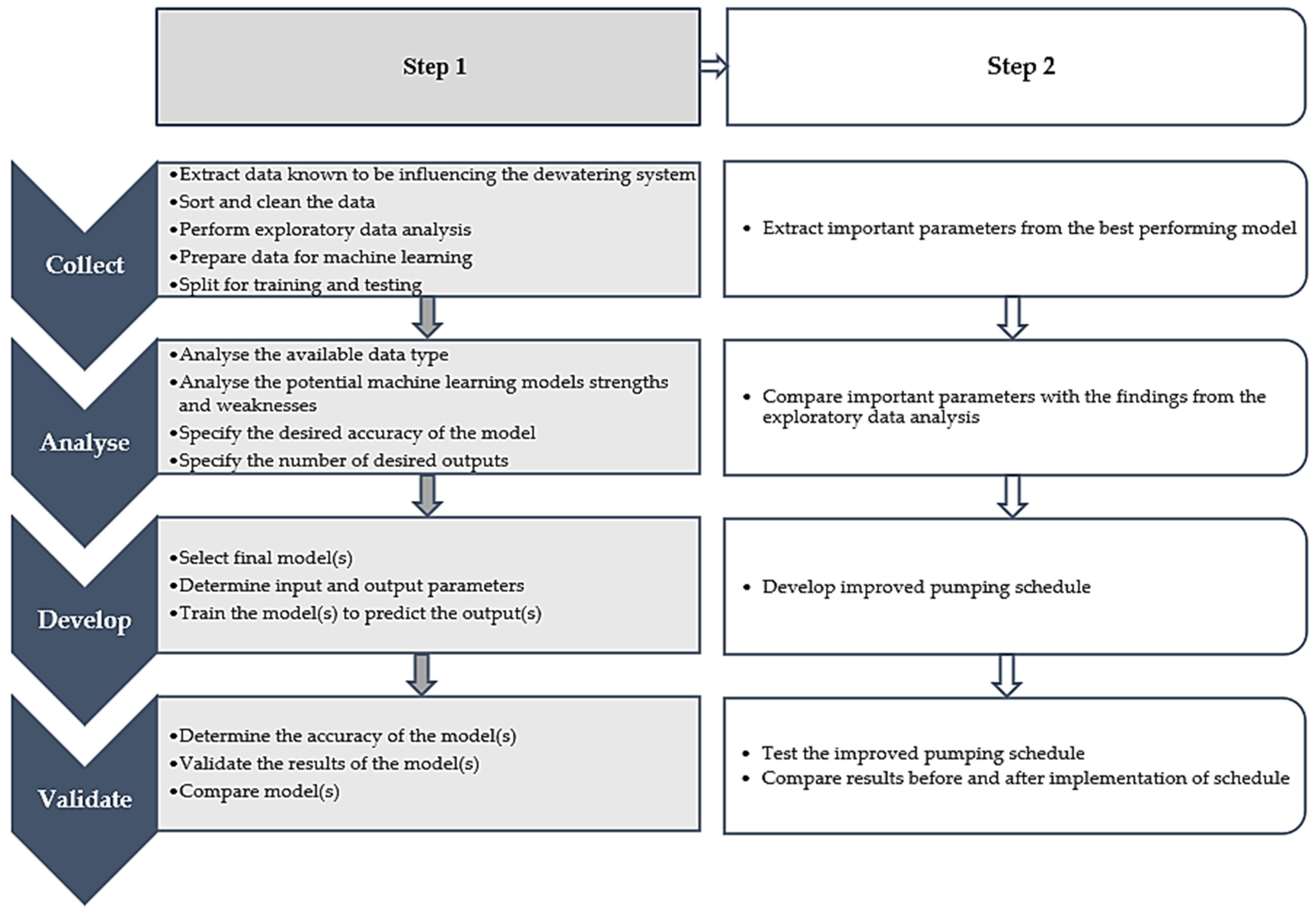
The primary focus of the developed method is to explore machine learning as an approach to identifying important parameters influencing pumping load shifts in a complex dewatering system of a deep-level mine. Figure 1 aims to describe the development of a solution that was applied in addressing the problem statement.

The four main steps to implement a solution were collecting, analysing, developing, and validating [29]. The focus of step 1 was on analysing a complex dewatering system in deep-level mines using advanced techniques such as machine learning algorithms. The emphasis of step 2 was to develop an improved schedule to test the efficacy of using machine learning models to address the problem statement.

Sahoo et al. [30] used Python to perform data cleaning, build a machine learning model, and visualise the study results. Predicting the power consumption during days with ideal pumping load shift was also achieved using Python programming to perform data cleaning, building machine learning models, and visualising the results of this study. The important features were extracted from the best-performing model to indicate important parameters that significantly affect the power consumption of a complex dewatering system during peak billing periods.

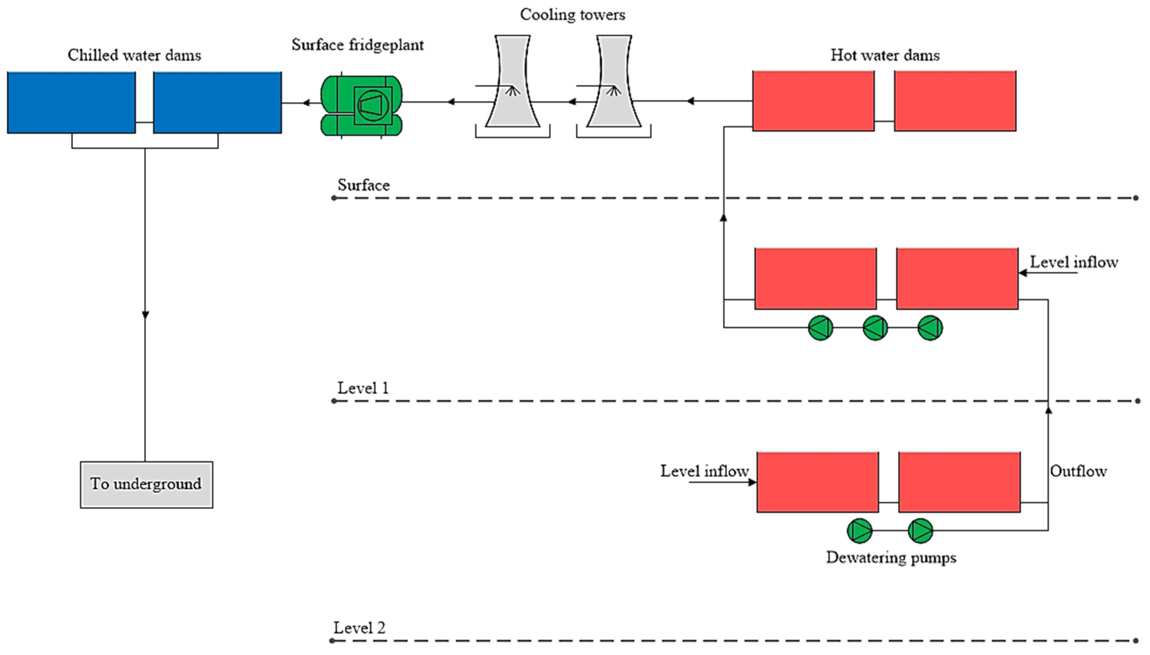
2.1. Complex Dewatering System of a Deep-Level Mine

A complex dewatering system in deep-level mines involves a cascading system of dams and pumps to move water from underground levels to the surface. The water is then cleaned, cooled, and returned underground for artificial cooling. The system incorporates data-acquiring components like dam level sensors, flow meters, and programmable logic controllers (PLCs). Data from this field equipment are transmitted to the PLC, which further communicates with industrial control systems like supervisory control and data acquisition (SCADA) for monitoring and management. The methodology was developed for a complex dewatering system with multiple working levels, dams, pumps, pipelines, and cooling systems, as depicted in Figure 2.

2.2. Data Collection

Data for the dewatering system were sourced from reports, observations, industrial control systems, and a real-time energy management systems database. Datasets from field equipment were typically stored in the SCADA or the historian. The initial step involved extracting data from these systems to establish a baseline before implementing any optimisation solutions. Validation procedures were employed to ensure the reliability and accuracy of the extracted data, focusing on factors such as zero values, flat-lining datasets, and unrealistic values [31]. Following validation, a baseline for power consumption was constructed.

2.3. Baselining

The baseline serves as a profile illustrating the energy usage trend under normal operating conditions. Baselining is a method used to establish a profile that defines a measured system’s demand over a specified period, ranging from 24 h to 12 months, depending on the analysis context [32]. For this manuscript, 12 months was employed to create both winter and summer baselines, further categorised into weekdays, Saturdays, and Sundays, due to differing energy consumption trends and billing tariff structures.

The analysis focused on weekday data, since weekdays are the only days that include peak billing periods, then averaged based on timestamps and seasons to generate winter and summer average power consumption profiles. The variance between power consumption profiles and the baselines was used to quantify the impact of the implemented energy management project. Additionally, the baseline profiles facilitated daily monitoring of system changes, with variations indicating factors such as production increases or system inefficiencies like water misuse or pipe leaks [33].

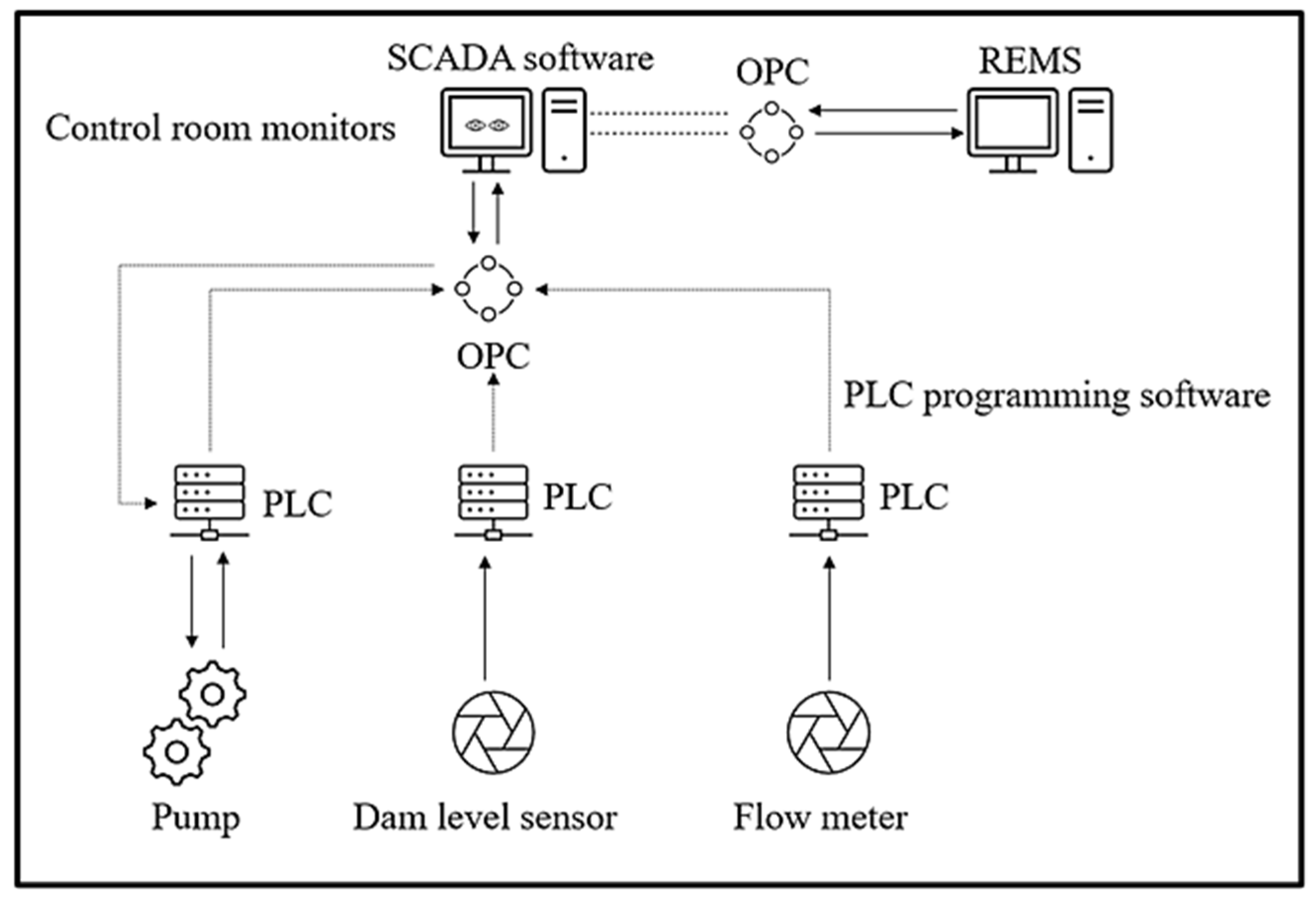
2.4. Real-Time Energy Management System (REMS)

A real-time energy management system (REMS) can automate the control of field equipment on surface and underground by sending signals to the SCADA system [34,35]. However, control operators often prefer manual control of critical equipment. In such cases, the REMS can send signals to the operators for guidance on starting or stopping pumps. The signal flow between SCADA, REMS, and field equipment is illustrated in Figure 3.

To optimise energy cost savings during peak billing hours, a load-shifting project was initiated using the REMS to minimise the number of pumps running [36]. Despite the benefits, the REMS may face challenges with sudden system changes, such as pump breakdowns. A thorough analysis of the dewatering system was conducted to enhance the baseline profile for more significant energy savings. Machine learning algorithms were employed to narrow down the systems or field equipment that required control, improving the potential for load shifting.

2.5. Data Preparation

Data acquisition marks the initial step in machine learning model building, involving gathering data from diverse sources and in various file formats. These formats, including pictures, text files, and Excel spreadsheets, need preprocessing to facilitate readability and analysis. Excel and programming languages like R and Python are commonly employed [37,38]. While Excel has limitations for large datasets, R and Python excel in handling them [38]. Python was utilised for data wrangling and building machine learning models in this context.

SCADA data were transformed into a data frame, and its statistical description was explored. Before constructing a machine learning model, expert knowledge was applied to clean, process, and analyse the data. Column names were renamed, and data were processed to eliminate anomalies like missing values for better comprehension. Statistical analysis provided additional insights into the complexities of the dewatering system. The quantitative data were then prepared for machine learning applications by ensuring that only the dataset from days where the pumping load shift was good was included in the data frame; that is, the average power consumption during peak billing periods was less than 20% of the maximum power consumption.

2.6. Computational and Machine Learning Models

Scikit-learn library in Python was used for multiple linear regression (MLR) model development. The dataset underwent preprocessing, including scaling and normalisation, using MinMax and Standard Scaler to address variable unit differences. Performance metrics like mean absolute error (MAE), mean absolute percentage error (MAPE), mean squared error (MSE), root mean squared error (RMSE), and the Pearson correlation coefficient ($R^2$) were introduced for model evaluation [39].

Cross-validation, specifically k-fold cross-validation, was employed to assess the model’s generalisation ability and prevent overfitting [40]. The extreme gradient boosting (XGBoost) model was then introduced as a non-linear alternative capable of handling complex relationships in input and output data. The process of developing the XGBoost model, including hyperparameter tuning using GridSearchCV, was detailed. Feature importance analysis was highlighted as crucial in understanding the model’s decision-making process and informing control strategies. The study concluded by emphasising the consideration of the dataset with successful load shifting for model evaluation and further analysis.

2.7. Implementation of Improved Pumping Schedule

The operation scheduling problem of a pumping system can be formulated as a cost optimisation problem, of which the objective is to maximise the energy cost saving while the system constraints are satisfied. In formulating the improved pumping schedule, 30 min intervals were used to avoid the repeated starting and stopping of pumps, since this can cause the pump to overheat and undergo excessive stress, which leads to premature failure [11], thus resulting in increased maintenance costs [41].

The historical data from REMS control during days where the pumping load shift was good and machine learning results were used to improve the pumping load shift. A schedule was devised from these data, whereby daily average profiles of water flow rates, pump energy consumption, and dam levels were analysed and used in 30 min intervals. Additionally, the most efficient pumps were suggested to be the only pumps that can be started during peak hours should a need arise to start a pump.

The schedule was then tested for a few days with experts monitoring the performance. When the schedule underperformed, the model was retrained, tested, and verified to increase the model’s accuracy. Once the performance was deemed good, the new schedule was implemented to achieve improved energy cost savings. The energy cost savings from the implemented schedule were calculated as the difference between energy cost savings from REMS control (before machine learning) and after the implementation of the machine learning model.

The area under the power consumption curve over a specific period is the energy consumption by the dewatering system. Since the cost of electricity differs throughout the day due to peak, standard, and off-peak billing periods, the total cost of energy consumption can be calculated as follows:

$$C_{pumping}={{\displaystyle \int }}_{t=0}^{t=48}P{\left(t\right)}_{baseline}\times T\left(t\right) dt$$

(1)

where $C_{pumping}$ is the electricity cost due to pumping, $P{\left(t\right)}_{baseline}$ is the baseline power consumption throughout the day in 30 min intervals as a function of time, and $T\left(t\right)$ is the tariff as a function of time. To estimate the cost impact of the REMS control and machine learning implementation, this equation can be represented as a matrix, as follows:

$$C_{pumping}={\left[\overline{E}\times \overline{T}\right]}_{baseline}$$

(2)

where $\overline{E}$ is the energy consumption matrix in $\mathrm{kWh}$ and $\overline{T}$ is the tariff matrix in $\mathrm{c}/\mathrm{kWh}$, such that the following are true:

$$\overline{E}=\left[\begin{array}{c}{E}_1\\ ⋮\\ E_{48}\end{array}\right].$$

(3)

$$\overline{T}=\left[\begin{array}{c}{T}_1\\ ⋮\\ T_{48}\end{array}\right]$$

(4)

The interval is from 1 to 48, since the time is from 00:00 to 23:30 over a day at 30 min intervals; thus, 48 data points. The energy cost savings from REMS control can then be represented as follows:

$$C_{savings\_1}={\left[\overline{E}\times \overline{T}\right]}_{baseline}-{\left[\overline{E}\times \overline{T}\right]}_{REMS}$$

(5)

and the energy cost savings as a result of this study can be quantified as follows:

$$C_{savings\_2}={\left[\overline{E}\times \overline{T}\right]}_{baseline}-{\left[\overline{E}\times \overline{T}\right]}_{REMS}-{\left[\overline{E}\times \overline{T}\right]}_{REMS\_ML}$$

(6)

where $\overline{T}$ is also a constant. The above formulation is a concise way to articulate improved energy cost savings.

3. Case Study: Application on a Complex Dewatering System of a Deep-Level Mine

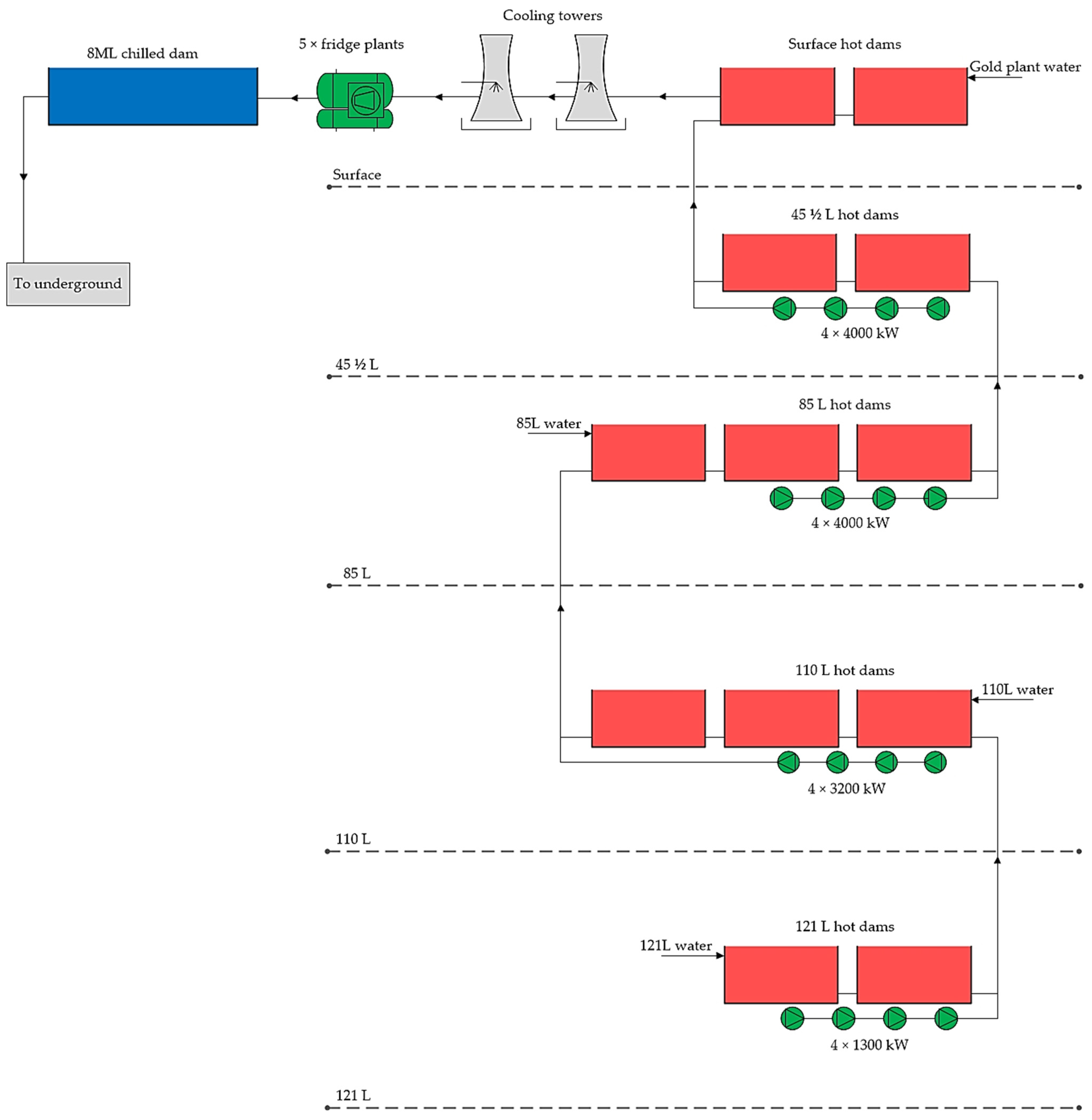
Figure 4 shows a simplified layout of the complex dewatering system of the case study mine. The mine is situated in the gold fields of the Witwatersrand Basin in South Africa. The complexity of Mine A is a result of the gold mine being one of the deepest mines in the world, with a depth greater than 4 km. Due to increasing temperatures underground, artificial cooling systems are required to ensure that the working conditions are safe for mine workers. In most cases, deep-level mines use water as a medium for heat transfer to cool down the air underground [42].

At Mine A, the water is cooled down to $3 °C$ using five industrial fridge plants on the surface. Once the water is cooled to the desired temperature, it is stored in a chilled dam with a volume of eight megalitres (8 ML dam). The 8 ML dam is a buffer dam to ensure that the chilled water demands underground are met throughout the day, as the demand is not constant, due to different mining activities conducted through different shifts [43]. The artificial cooling systems used at Mine A are bulk air coolers (BACs) and mobile cooling units (MCUs).

The chilled water is passed through a series of coils in BACs and MCUs, and the hot underground air is blown into the artificial cooling system using fans. This results in heat loss in the air and heat gain in the water. The warm water is then further used for mining activities such as cooling down the drill bits of the rock drills, dust suppression, moving the ore fines, etc. The hot water then moves through a series of sumps, filters, and spindle pumps, until it reaches the dewatering dams, which are also referred to as hot dams.

The case study mine is divided into levels. The naming convention of the levels is derived from the British imperial and United States customary system of measurement, feet (ft). The water used on and below 12,100 ft or 3.69 km underground is stored on the 121 level (121 L), which is 12,100 ft underground. The level depicts the depth of the area underground; hence, 121 L is $121\times {10}^2$ ft below surface. The hot water is pumped through a cascading system of dams and pumps until it reaches the surface, where it is cleaned and cooled.

For Mine A to adhere to Mine Health and Safety Act regulations regarding flooding of the mine, prevention of flooding, flooding precautions, drains and rock passes, and communication to surface, the dewatering system consists of many dams and pumps (see

Table 1. Dewatering system dams of Mine A.

Area	System Name	Quantity	Total Capacity (ML)
Surface	Round and square dam	2	9
45.5 L	45.5 L hot dam	2	4.8
85 L	85 L hot dam	3	4.8
110 L	110 L hot dam	3	4.8
121 L	121 L hot dam	2	4.8

and

Table 2. Dewatering system pumps of Mine A.

Level	System Name	Quantity	Flow per System (L/s)	Power Rating (kW)
45.5 L	45.5 L pump	4	245	4000
85 L	85 L pump	4	230	4000
110 L	110 L pump	4	270	3200
121 L	121 L pump	4	245	1300

).

The dewatering system is equipped with actuators, sensors, and flow meters to allow for the operation of valves and pumps from surface using the industrial control system. The operators can observe and monitor the conditions of field equipment on the surface and underground from the SCADA system. Decisions can then be made to start and stop the pumps, open and close flow control valves, etc., to ensure safe mining and meet underground demands. The AVEVA Plant SCADA 2020v2 software allows for alarms to be set for value limits and trends of previous data to be viewed to ease the control and condition monitoring process. Previous data of the tags are stored in a historical database to allow for the analysis of the data at a later stage when needed.

The appointed engineers and management of Mine A devised a pumping and flooding procedure that needs to be adhered to. This process and procedure (P&P) document was compiled as a guideline to manage surface and underground pumping. The objective of the pumping and flooding procedure document is to prevent harm to personnel, damage to property, loss of production, and to conserve energy. The control room operators mostly use their discretion from training and experience to adhere to the document.

From the document, a schedule was devised for the operators as a guideline for the dewatering process. Among others, the operator’s supervisor can access the SCADA software remotely using an OPC connection. Client servers can use an OPC connection to extract historical data from the SCADA software historian.

3.1. Data Collection

The power consumption data of the dewatering system were extracted from one of the historians of Mine A. The historian allows for data extraction in different formats such as Excel, csv, and pdf files. The preferred method of extraction was the Excel format, since the extracted data ranged from June 2019 to May 2021 and were not too large for Excel. The data were extracted in 30 min intervals and consisted of 21,648 rows and 83 columns. The power consumption data were filtered to only include weekdays, to form a weekday baseline. Since it is imperative that the data correlate with Eskom data for billing purposes, it can be assumed that the data were of high quality.

A quick statistical analysis was performed on the data to check the minimum, maximum, and average power consumption by the dewatering system. A rule of thumb for estimating the power consumption by a pump is as follows:

$$P_{theoretical}=\eta \times P_{design}$$

(7)

where $P_{theoretical}$ is the theoretical power consumption, $\eta$ is the pump efficiency, and $P_{design}$ is the design power rating.

Table 3. Theoretical and actual power consumption by the dewatering system of Mine A.

Theoretical Power (kW)			Actual Power (kW)
Minimum	Average	Maximum	Minimum	Average	Maximum
0	21,000	42,000	3930	17,577	25,803

shows the theoretical and actual power consumption of the dewatering pumps.

Theoretically, if no pump is running, the energy usage will be close to 0 kWh. However, as seen in Table 3, there is never a 30 min interval where no pump is running during the week, due to the complexity of the system and the rate at which the dewatering dams rise. From Equation (7), the maximum theoretical energy usage by the dewatering pumps of Mine A is approximately 42,000 kWh. However, when investigating the dewatering system, it was found that the pumps are connected to two-meter panels, namely MP11 and MP12, which are limited to 17,000 kWh each or 34,000 kWh in total without tripping. It is the responsibility of the control room operators to ensure that the mine does not flood, and the meter panels do not trip; hence, a total maximum energy usage of 25,803 kWh is observed from the dataset of the dewatering pumps.

3.2. Baselining

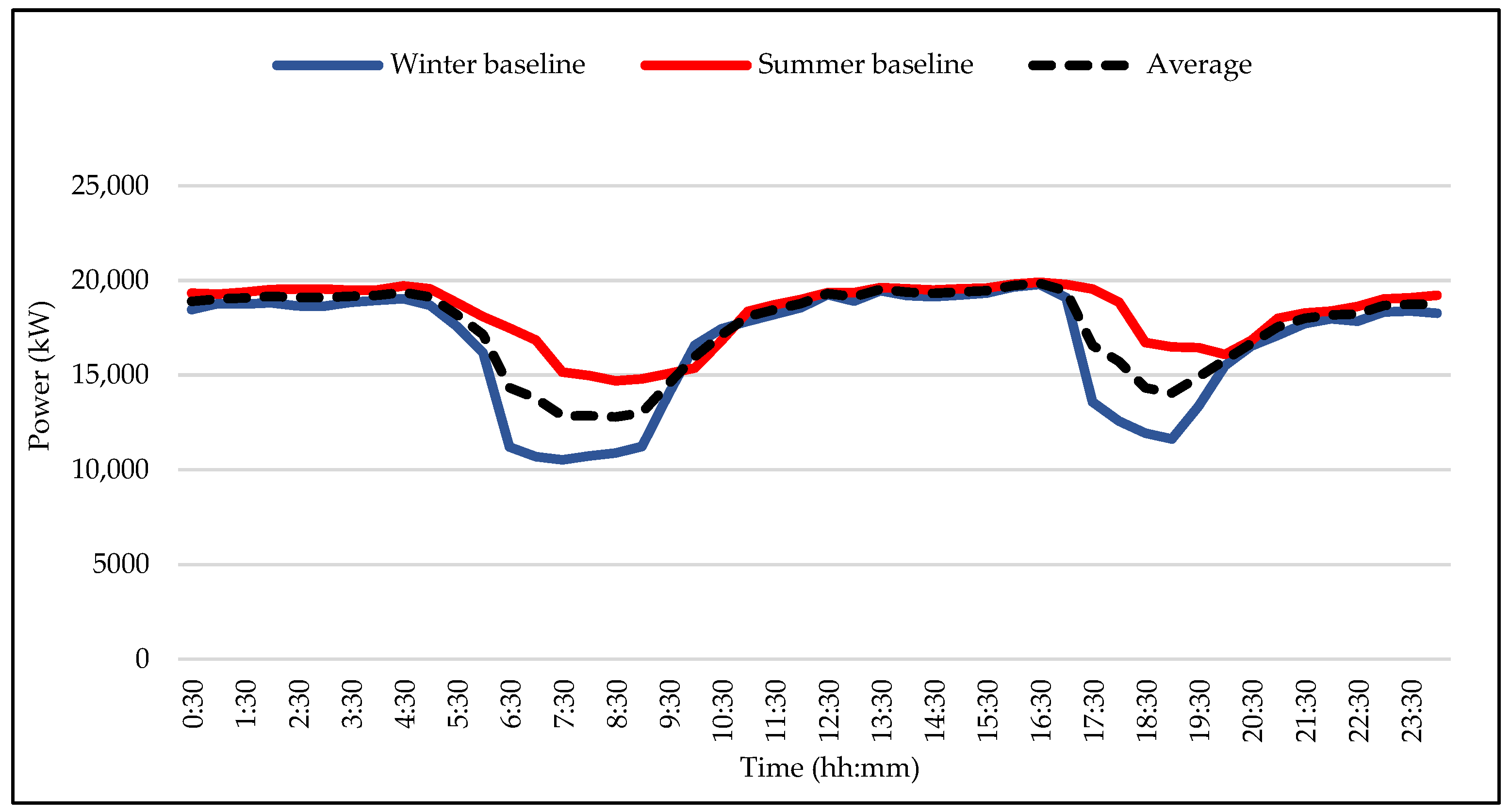
The average energy usage from June 2019 to May 2021 was 17,577 kWh. Since Eskom months are divided into high demand season (winter), which is from June to August, and low demand season (summer), which is from September to May, Figure 5 shows the average power consumption during high demand season (June 2019–August 2019 and June 2020–August 2020) and low demand season (September 2019–May 2020 and September 2020–May 2021), which formed the baseline for winter and summer, respectively.

The baselines in Figure 5 show the trend of energy usage under business-as-usual (BAU) conditions. Due to the nature of dewatering system operations and Eskom tariffs, baselines have been determined separately for winter and summer months, aligned with the tariff structure of Eskom for winter and summer seasons. The baselines need to be adjusted whenever energy performance indicators no longer reflect the system’s energy use or there are major changes to the dewatering process, operational patterns, or energy systems.

3.3. Energy Management System Results

An OPC connection can be established between SCADA and the REMS [44]. This connection can be used for automation of the dewatering system or to allow for alarms and signals to be sent between the SCADA and the REMS. The demand side management (DSM) initiative to implement a pumping load shift was initiated at the case study mine in June 2021 to lower operational costs and realise energy cost savings. REMS v9.1.4.0 software was used to send signals to the SCADA to notify operators which pump to switch on or off. The method followed in programming the REMS was looking into dam levels, the average rate of increase in the dam level, pump availability, dewatering system constraints, and sending a binary signal to SCADA based on predicted dam levels.

The objective was to optimise energy cost savings by shifting most of the pumping load out of Eskom tariff peak hours to standard and off-peak hours. The simulation revealed that, based on real-time data, it is feasible to implement a load shifting initiative on the dewatering system. Figure 6 shows load shifting results of the dewatering system calculated by the REMS.

REMS simulation results allowed the case study mine to achieve USD 6695 energy cost savings on a winter day; however, as seen in Figure 6, pumps had to be started prematurely due to rising dam levels. Additionally, one pump on 121 L experienced a breakdown and was unavailable for eight consecutive months. Even though the energy cost savings target was achieved, the pumping load shift can be further improved by learning from previous data, predicting power consumption based on previous data, realising which systems greatly influence the dewatering system, and better controlling these systems instead of reacting only to dam levels.

Additionally, it was realised that, during days when flow meters were faulty, the REMS simulation tended to perform worse, since it depended on real-time data to make accurate predictions.

3.4. Machine Learning Results

The objective of the pumping load shift initiative was redefined to further improve the load shifting performance and reduce operational costs. The new objective was then to improve the pumping load shift of the complex dewatering system using machine learning to overcome the constraints of mathematical and simulation models.

From the extracted dataset, the days where the pumping load shift performance was good were rigorously analysed. The data initially extracted contained 21,649 rows and 83 columns and was filtered to only include the data where the power consumption during morning and evening peak was less than 4000 kW on average, which equates to only one pump running on either 45.5 L or 85 L. This resulted in 3552 rows and 83 columns. The significant reduction in data points showed that the simulation software was insufficient for ensuring good pumping load shifts during most days. The actual minimum, average, and maximum power consumption of the dewatering system during winter peak hours of the reduced dataset were 0 kW, 3870 kW, and 15,482 kW, respectively. The average power consumption during peak was below 4000 kW, but the maximum consumption was considerably higher. This was taken into consideration when further analysing the reduced dataset.

3.4.1. Data Organising and Pre-Processing

Python programming was used for the data pre-processing, cleaning, and machine learning model building. This process was achieved using a Jupyter notebook v7.0.8. Jupyter notebook is a web application that supports the fast creation of literate programming documents that combine code, text, and execution results with visualisations in an interactive manner [45].

The NumPy, Pandas, Matplotlib, Seaborn, and SciPy libraries were imported into the Jupyter notebook to organise and pre-process the dataset. The csv file was then converted to a data frame. Unnecessary or duplicated columns, such as Timestamp, Date, Months-Calendar, Months-Eskom, Time-Hrs, Year, Month, and Day, were removed from the data frame. The data were pre-processed to produce a new data frame by renaming the columns to more readable column names and combining the water flows, since two pipes are used to deliver water from level to level. Hence, only one column represented water flow from a specific dam.

The data of the pumps were then split according to the electrical meter panels they are connected to (MP11 and MP12), since the meter panels trip if overloaded. A count of missing data points from important columns, such as pump status, was calculated to clean the data. Additionally, rows that had too many missing essential data points were removed, and data points with a few missing important data points were populated using linear interpolation. A statistical table was then produced to see if the remaining dataset made sense from an expert perspective.

The table included the total count of the data points, mean, standard deviation, and five-number summary of the dataset. From being familiar with the case study mine, the unrealistic data points such as dam levels going below 15% were removed from the dataset. The operators confirmed that the dam level is consistently above 15%, since mud usually builds up below 15% of the dam level. If the suction of the pump delivers large quantities of mud, the mud can damage the pump, since it was not designed to pump mud.

Supervised machine learning algorithms were then used to predict the power consumption based on the dewatering system parameters. Once the machine learning model predicts the power consumption to an acceptable level of accuracy, a feature importance table can then be produced to see which parameters highly influence the load shifting potential. Since 3 h in the morning and 2 h in the evening are billing peak hours, better control of important parameters during the 19 h of dam preparations can allow operators to better perform the pumping load shift.

3.4.2. Multivariate Linear Regression Model

Linear regression (LR) is a standard statistical data analysis technique that was used to predict power consumption. Instead of fitting a linear regression model for every input to every output, multivariate linear regression (MLR) accommodates multiple inputs and a single output to produce a single model. Hence, for power consumption by the dewatering system, two models were computed. One model was expected to predict the power consumption based on the time of use, dam levels, dam temperatures, fridge plant flows, and dewatering pump statuses. The other model was expected to do the same without the dewatering pump statuses.

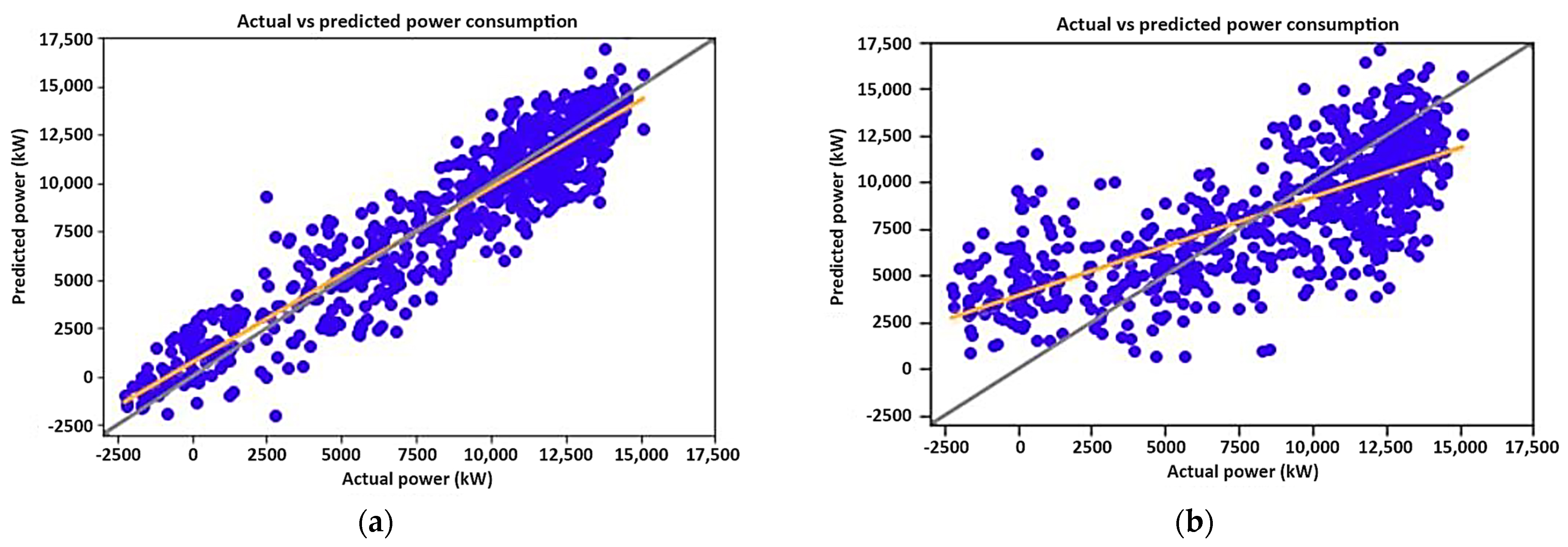
A linear regression model assumes that there is a linear relationship between the inputs and the outputs, and the results of the two models are presented in Figure 7.

Figure 7 shows the performance of the MLR model in predicting the power consumption as scatter plots. The orange line among the scatter points is the line of best fit, which is the best approximation of the scatter points. The grey diagonal line is a one-to-one line that shows the best prediction if the line of best fit or scatter points were to perfectly lie on it. The closer the line of best fit and the scatter points are to the one-to-one line, the better the performance of the model.

Figure 7a shows that the model performed well when given pump statuses as inputs with an $R^2$ value of 0.88, while it performed poorly without pump statuses with an $R^2$ value of 0.53. This is due to the dewatering system’s power consumption directly being caused by pump statuses, hence the linear relationship with power consumption. Figure 7b shows that the relationship between other system parameters and actual power consumption is non-linear.

3.4.3. Extreme Gradient Boosting Model

An XGBoost model was then developed using the same dataset but with a different approach for assuming linearity between input and output parameters. The XGBoost model was optimised by tuning the hyperparameters. The hyperparameters that were tuned to improve the performance of the model are described below (See

Table 4. XGBoost hyperparameters tuned (adapted from [46]).

Hyperparameter	Description
learning_rate	Rate at which the model upgrades its weights
max_depth	Maximum depth of the tree
min_child_weight	Minimum sum of weights of all observations required in a child leaf
nthread	Number of cores in the computer system for processing
sub_sample	Ratio of number of samples from total training samples used in each tree

).

GridSearchCV was used in tuning the hyperparameters with five folds. A set of possible values for each parameter was provided for the grid search, and the best combination of hyperparameters was produced as an output from the function. The values provided to GridSearchCV were as follows:

Considered hyperparameters: {‘learning_rate’: [0.03, 0.05, 0.1], ‘max_depth’: [3, 5, 7, 10], ‘min_child_weight’: [2, 4, 6], ‘nthread’: [4], ‘subsample’: [0.5, 0.7, 0.9], ‘colsample_bytree’: [0.6, 0.7, 0.8], ‘n_estimators’: [300,500,700]}

and the results from GridSearchCV were as follows:

Best hyperparameters: {[‘colsample_bytree’: 0.6, ‘learning_rate’: 0.05, ‘max_depth’: 10, ‘min_child_weigh’: 4, ‘n_estimators’: 300, ‘nthread’: 4, ‘subsample’: 0.7]}

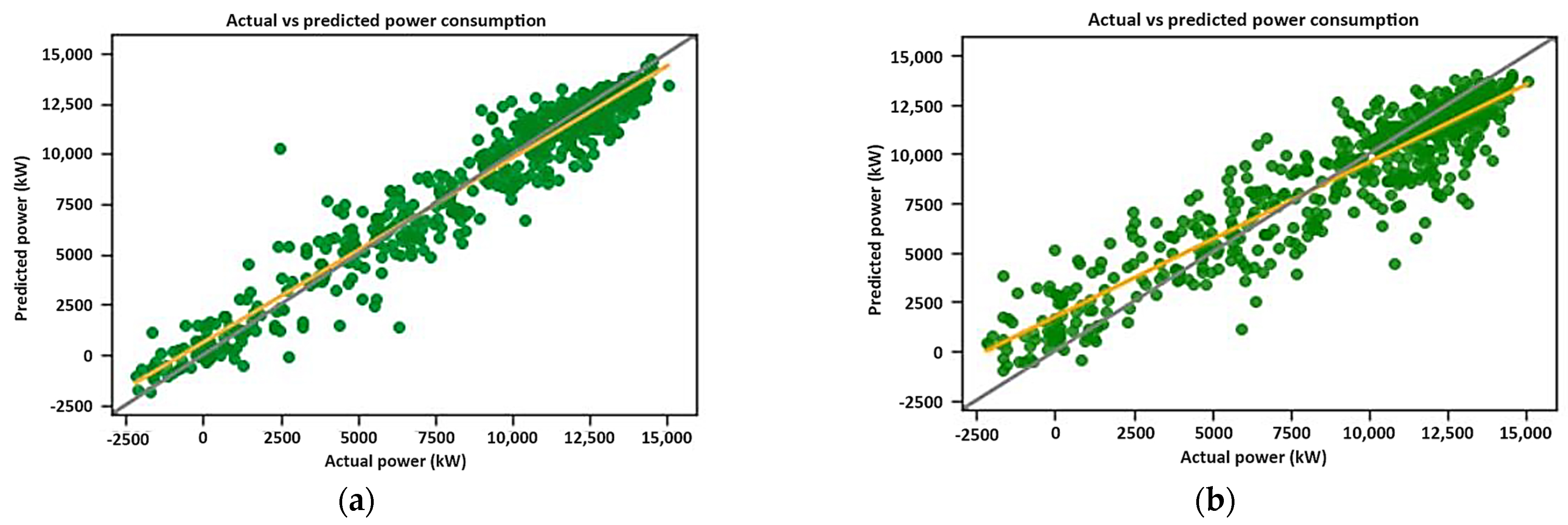
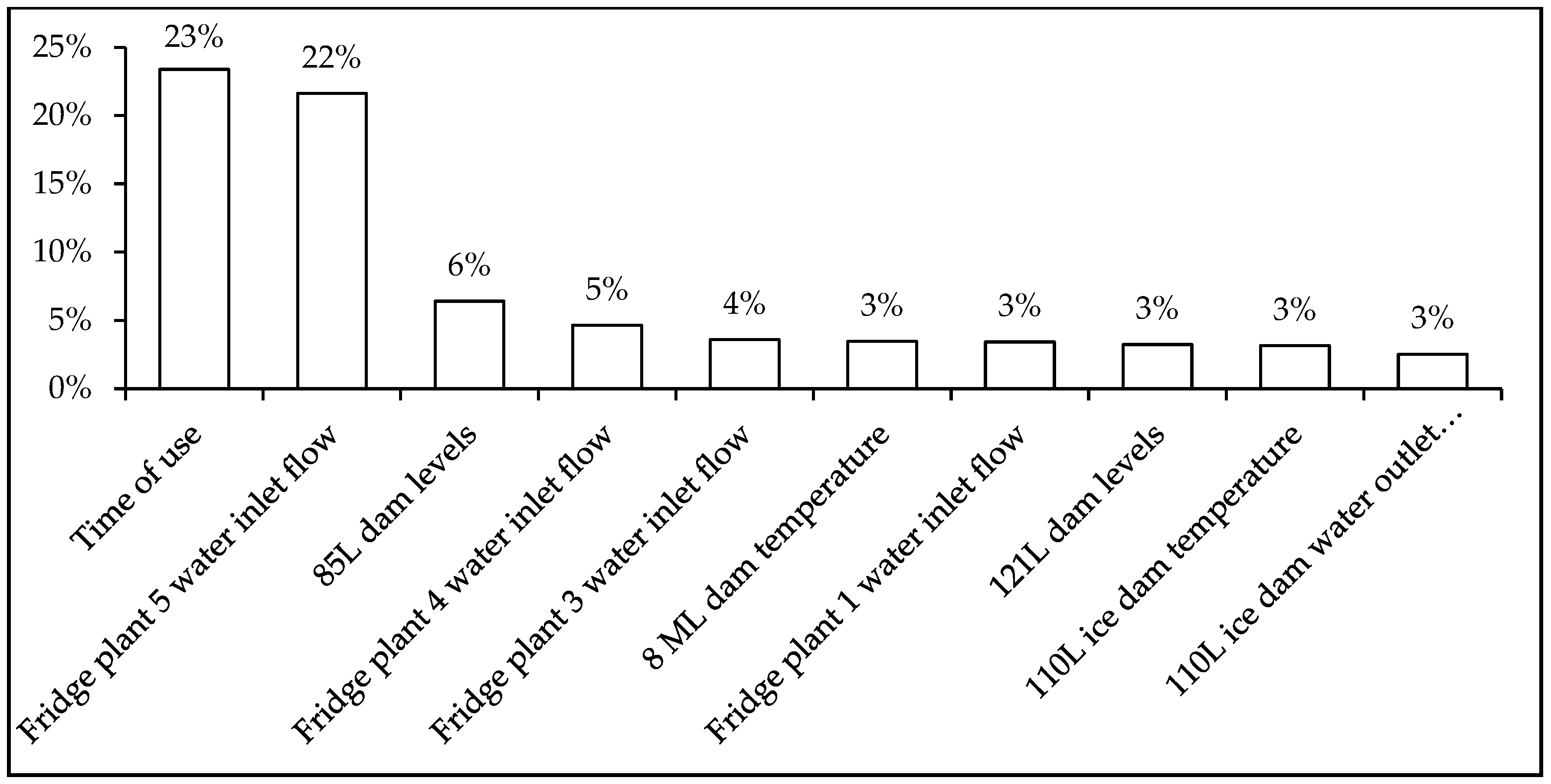
Similarly to the linear regression model, two XGBoost models were built, and the results are represented in Figure 8. Figure 8a,b shows that both models performed well, with $R^2$ values of 0.94 and 0.87, respectively. Looking at the weights of the input parameters, 10 input parameters were identified as important when excluding dewatering pumps and were plotted in Figure 9.

From observation, feature importance shows the time of use, fridge plant inlet flow or surface hot dam outlet flow, and the 85 L dam level being the most important parameters. Since Mine A was already load shifting, time of use was expected to be part of the important features. The operation scheduling of the pumps has a substantial influence on energy costs, since the TOU tariff is different throughout the day [44,47].

Additionally, from feature importance, the inlet flow from the fridge plants is what is draining the round and square dams; hence, low levels of the round and square dams force the operators to start the dewatering pumps. An interesting observation is that the 85 L dam levels are the third important feature. Upon investigation, it was found that two pumps on 85 L had been tampered with. The impellers of these pumps were cut and reduced, since the motors of the pumps tended to overheat regularly. The literature shows that reducing the diameter of a pump impeller reduces the flow rate, head, and power consumption [48].

Furthermore, the 8 ML dam temperature, 121 L dam levels, 110 L ice dam temperature, and 110 L ice dam outlet flow were also found to be the most important parameters influencing a good pumping load shift. The 8 ML dam temperature is the final coldest temperature of the water before it is distributed underground. It is imperative that the overall impact of underground cooling systems cool down the working areas below 32.5/37 °C (wet-bulb/dry-bulb) temperatures to comply with the legal thermal stress limits [49]. To ensure that the artificial cooling system provides sufficient cooling, the dam needs to be as cold as possible without forming ice in the pipes or freezing the pipes.

121 L is the lowest level with sufficiently big pumps to ensure the mine does not flood. Additionally, the water from the neighbouring mine is dewatered from 121 L. However, according to experts, Mine A was not initially designed to pump water from other mines.

The 110 L ice dam is the most important dam that ensures safe mining. The temperature of the 110 L ice dam determines the maximum water temperature of the underground cooling cars below 110 L. If the dam temperature is above the desired temperature, some of the water from the artificial cooling system is distributed to the dewatering dams instead of the ice dam to ensure working areas are below the legal thermal stress limits. This increases the amount of water that needs to be dewatered.

From this insight, time of use, 45.5 L pumps, 85 L pumps, and 121 L pumps were identified as the highest priorities. Time of use determines the cost savings, 45.5 L pumps determine the level of the round and square dams, 85 L pumps are the weakest link due to reduced impeller sizes, and 121 L pumps are under strain due to additional water from the neighbouring mine.

3.5. Improved Pumping Schedule

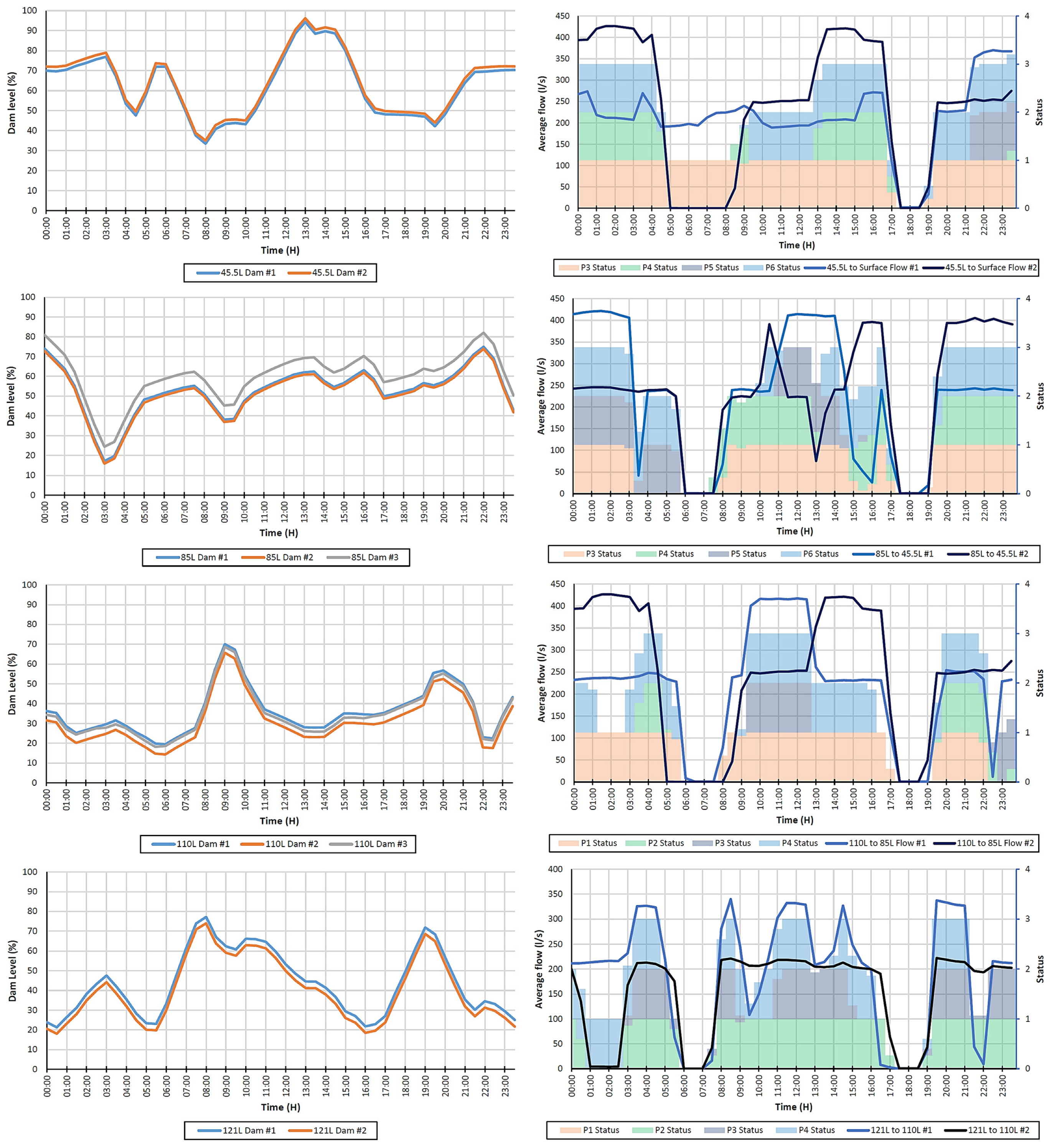
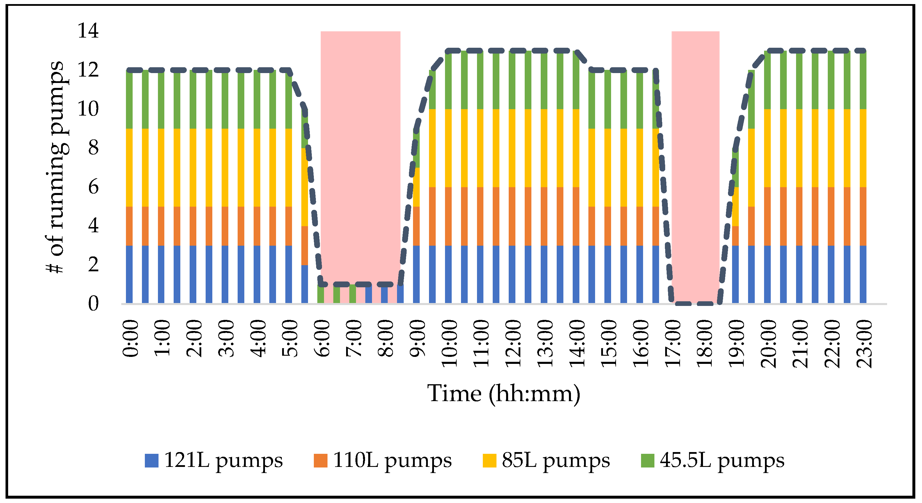
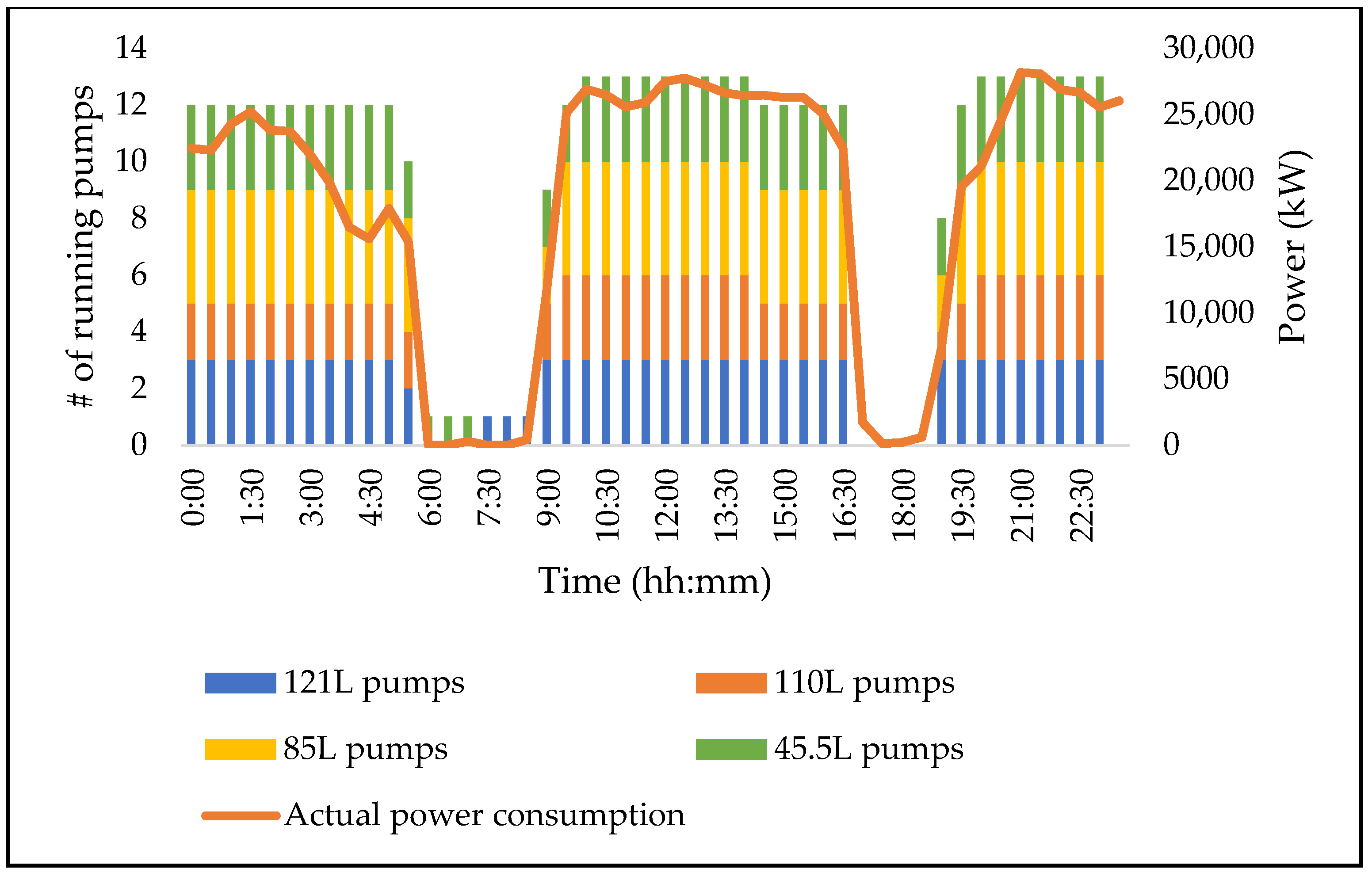
A pumping schedule was then devised based on this analysis of the pumping performance when the pumping load shift performed well. Figure 10 shows a graphical depiction of the proposed pumping schedule.

The new schedule suggested that one pump on 45.5 L must run for 30 min and then be followed by one pump on 121 L during the morning peak. This is due to the presence of power generating systems such as turbines and pumps in reverse operation, also referred to as pump-as-turbine (PAT), present at Mine A. The generated power cancels out the power consumed by these pumps during peak. The new schedule was then trialled for a day where no major breakdowns were present.

The trial was a success, with minor deviations from the schedule between 03:00 and 05:00 in the morning, as shown in Figure 11. The deviation was a result of one 110 L pump that tripped consistently due to high vibrations. As a safety feature, the instrumentation trips the pump to protect the pump from major damage. The deviation, however, had minor to no impact on the load shifting potential, since 110 L hot dams can easily be emptied. This can also be noticed from the results of the machine learning models and the feature importance graph in Figure 9, as the running statuses of 110 L pumps are not part of the top 10 input parameters highly influencing the pumping load shift.

Apart from the deviation between 03:00 and 05:00 in the morning, the operators followed the new schedule as intended, to ensure that the trial results were a true reflection of the schedule’s potential. From the performance of the trial, the cost savings for the day amounted to USD 9451. Furthermore, the load shifting performance greatly improved, as power consumption was close to zero during peak tariff hours.

The new schedule was then approved and distributed to the operators to officially follow and give feedback. The new schedule included additional information such as specific pumps to start should there be unprecedented issues such as a breakdown and the sequence in which to start the suggested pumps. This insight was previously not given to the operators; hence, the operators would tend to partially ignore pumping load shifts in the event of a crisis. 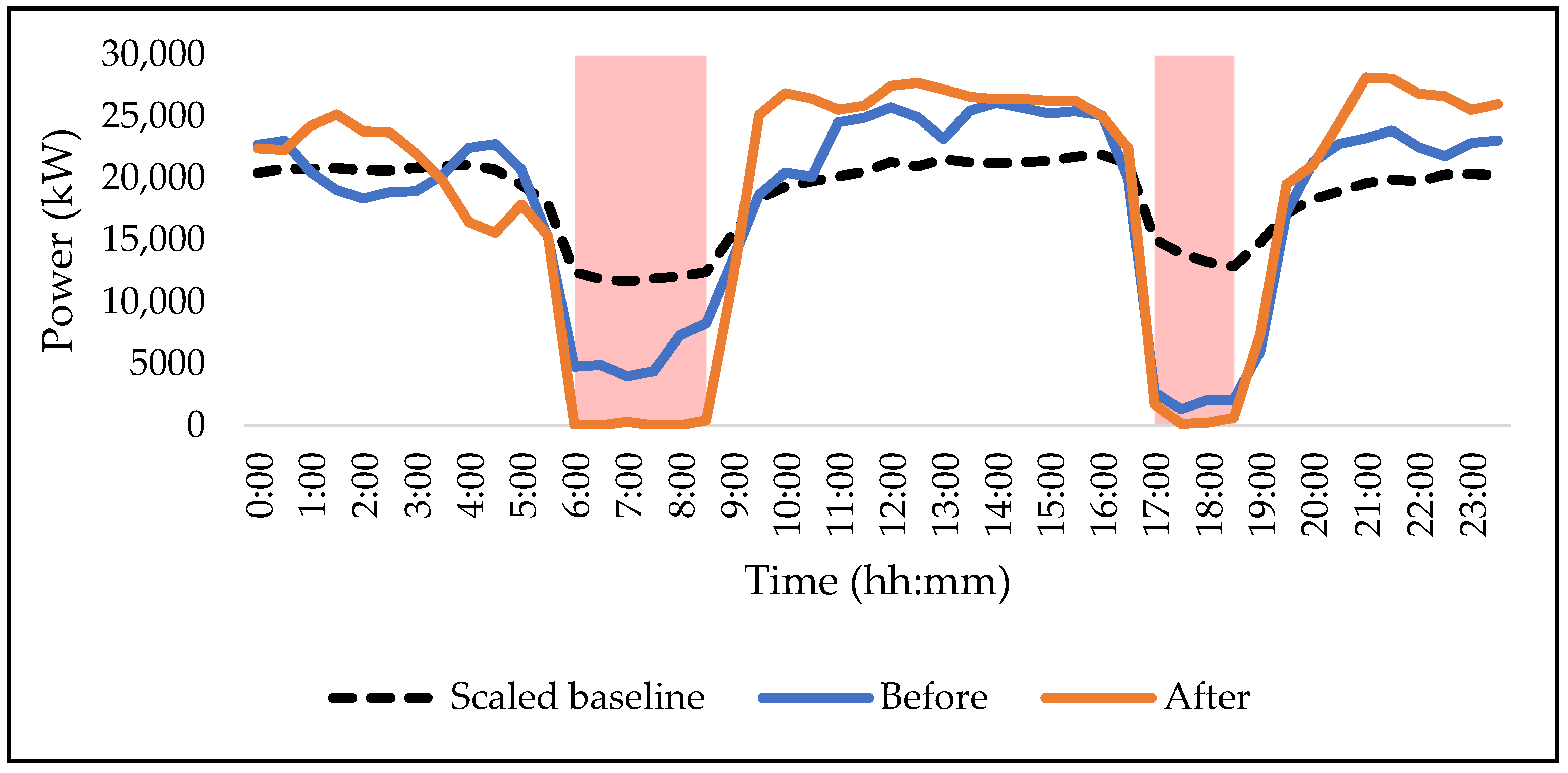Figure 12 shows the average weekly performance of the pumping load shift after machine learning insights.

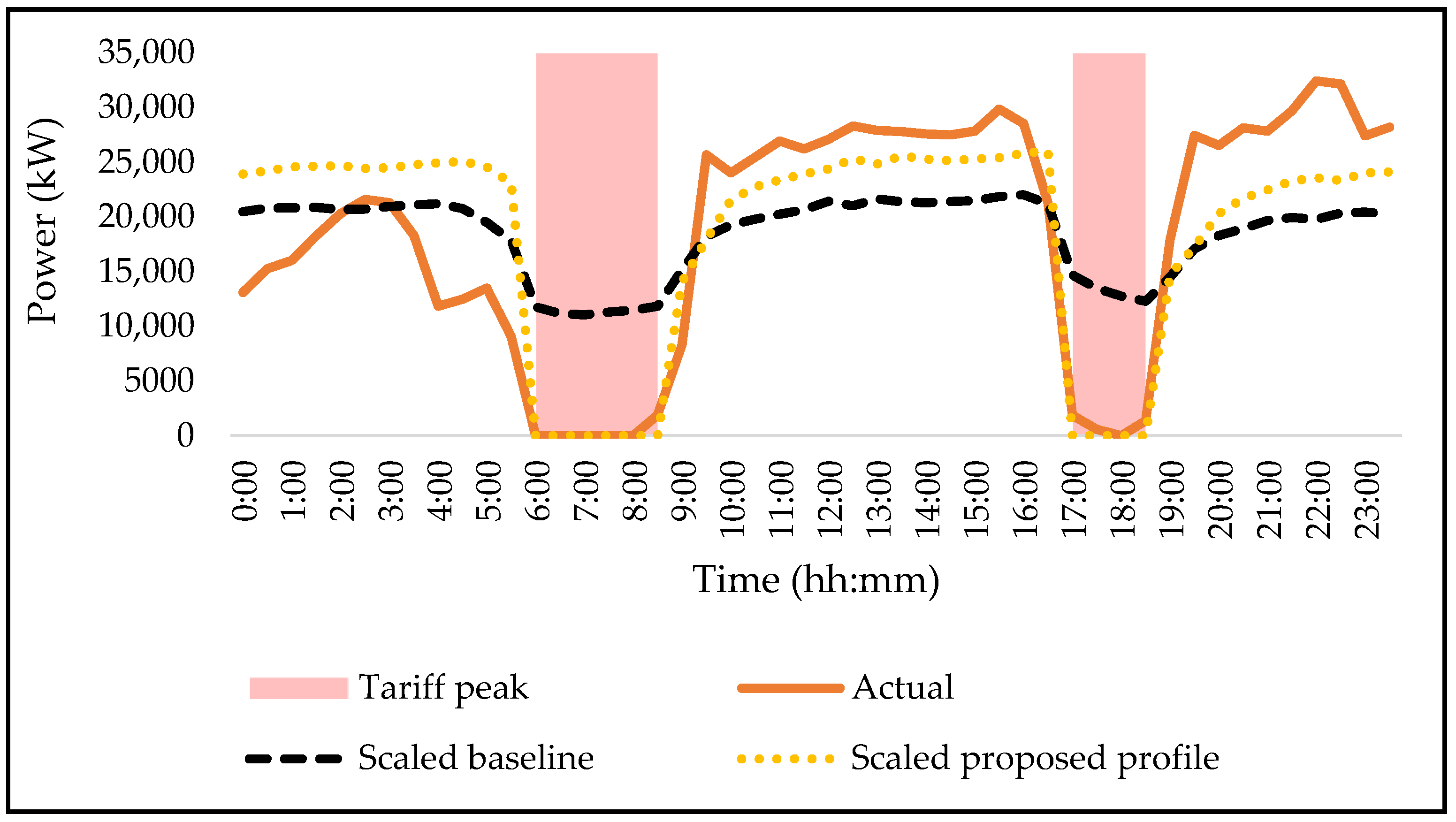
Additional savings of USD 21,548, which were previously missed, were realised after one week. This equates to an estimated additional saving of USD 255,000 per annum at Mine A during the winter season. Since correlation does not necessarily mean causation, Figure 13 was produced to highlight causality.

Figure 13 shows that the proposed running status of the dewatering pumps directly aligned with the power consumption by the system, with minor deviations. The results of Figure 12 and Figure 13 show practical benefits for the electricity grid since, during peak demand, the electricity usage by the mine’s dewatering system was minimal. Additionally, these figures also show financial benefits for the mining industry, since the energy cost savings were improved, thus improving the mine’s profitability.

Hasan et al. [50] tested a combination of different machine learning algorithms as five different ensemble methods to reach a classification accuracy of 89% and concluded that the results indicated that artificial intelligence (AI) could potentially be used to monitor and control mine dewatering systems. In this study, two different machine learning algorithms were tested to reach a predictive accuracy of 94%.

Important features were extracted from the best-performing machine learning model to reduce the optimisation scope of the dewatering system parameters. Additionally, the insight from machine learning improved the energy cost savings at the case study mine. These results indicate that machine learning, which is a subset of AI, can potentially be used to improve control of the mine’s dewatering system, regardless of the complexity of the system. Furthermore, Hyder et al. [51] posed research questions regarding the potential uses of AI and autonomous technologies in the mining industry, and the results of this study confirmed the potential of the use of AI in improving energy cost savings.

4. Conclusions

In this study, supervised machine learning models were employed to identify the 10 most significant subsystems/parameters influencing the energy costs associated with dewatering operations in deep-level mines. Leveraging insights gained from these models, measures were implemented to enhance the control of critical parameters, thus optimising the pumping load shift within a complex dewatering system.

The first model, MLR, was built to predict the power consumption of the dewatering system when the load shifting was well executed. The model performed well when pump running statuses were included as inputs to the model, resulting in an $R^2$ value of 0.88. This is due to the dewatering system’s power consumption directly being caused by the pump statuses, explaining the linear relationship with power consumption. Conversely, without pump statuses as inputs, the model’s predictive capability diminished, resulting in an $R^2$ value of 0.53. The poor performance of the second model showed that the relationship between other system parameters and actual power consumption was non-linear. This resulted in a second model being built. The literature has shown attractive features of the XGBoost model, which was therefore chosen to be the second model.

The XGBoost model demonstrated robust performance, achieving $R^2$ values of 0.94 and 0.87, with and without pump running statuses, respectively. By analysing input parameter weights, crucial factors affecting pumping load shift were identified, facilitating the development of an optimised pumping schedule. The implementation of this schedule resulted in substantial energy cost savings, amounting to USD 9451 during initial testing and an additional USD 21,548 over a one-week period following approval. The implications of these findings extend beyond immediate cost savings, with potential annual savings estimated at USD 255,000 during winter seasons.

Additionally, feature importance findings were found to be interpretable and corresponding to real world observations. The feature importance findings included pumps that are the weakest link in the dewatering system of the case study mine, due to reduced impeller sizes. This addresses the common concern that black box machine learning models are uninterpretable and therefore not suited for practical applications. In this case, the feature importance technique provided real world insights into the system.

The adoption of a case study methodology and quantitative approach proved instrumental in realising these improved energy cost savings, underlining the significance of identifying key parameters within complex dewatering systems. This approach not only enhances cost-effectiveness but also ensures consistency in energy savings over time.

Furthermore, the study highlights the limitations of traditional expert knowledge and simulation models in addressing the complexities inherent in dewatering systems. The transition to machine learning techniques offers a promising avenue for enhancing energy cost savings in deep level mining operations, thereby benefiting both the mining industry and broader energy grid sustainability.

Addressing these challenges contributes to the existing literature and fosters a deeper understanding of complex dewatering systems, paving the way for future advancements in energy management. The success of the study showed that machine learning techniques can be used to improve energy cost savings in complex dewatering systems of deep-level mines.