Ground Subsidence above Salt Caverns for Energy Storage: A Comparison of Prediction Methods with Emphasis on Convergence and Asymmetry

Abstract

Mining-induced subsidence can have significant environmental and infrastructural impacts, making subsidence engineering a crucial consideration. However, the unique nature of salt caverns and the increasing demand for reliable subsidence prediction models in the context of energy storage require special attention. This study provides a comparative analysis of existing prediction models and highlights their advantages and disadvantages to determine the most appropriate approach. The study primarily focuses on theoretically developing an empirical influence function for asymmetrical subsidence prediction. It significantly contributes to the field by correcting and extending the existing method, providing a generalized solution applicable to any type of asymmetrical distribution around the cavern. Future research directions include implementing the proposed model in relation to real-world data. The insights gained from this study can help advance subsidence prediction models in the field of salt cavern energy storage, addressing a significant need in the industry.

1. Introduction

Salt caverns are artificially constructed cavities in a salt formation. There are various methods of salt exploitation, but this study specifically focuses on salt caverns used for storing gas and liquids that are constructed through the leaching method. The mining method involves drilling a well into the rock salt with a diameter of d < 1 m. Several pipes are installed in this well and bonded with cement to the surrounding rock. During the solution mining process, water is injected to dissolve the salt. The produced brine is then transported to the surface [1]. Salt caverns are not only a source of NaCl, but they are also used as storage repositories for liquids and gas. In Germany, they are used for storing large quantities of natural gas (24% of all gas reserves). The reason for the popularity of the type of storage projects is the high flexibility of charging and discharging the gas [2]. A current focus in research is the investigation of the suitability of salt caverns to store hydrogen [3].

The void constructed during the leaching process and later used for energy storage leads to a destruction of the force balance in the surrounding rock mass and results in deformation, manifested by the cavern convergence. The deformation is the reason for ground subsidence. Surface deformations, such as tilt, tension, or compression, can negatively affect objects on the surface, e.g., houses of media pipes, or they can lead to degradation of land quality. To assess the impact on the environment, prevent the damage of objects, or estimate fair compensation, precise ground movement prediction methods are needed.

There are several prediction methods established in practice. This contribution aims to review the main features of the currently used methods in Europe and to estimate their further potential.

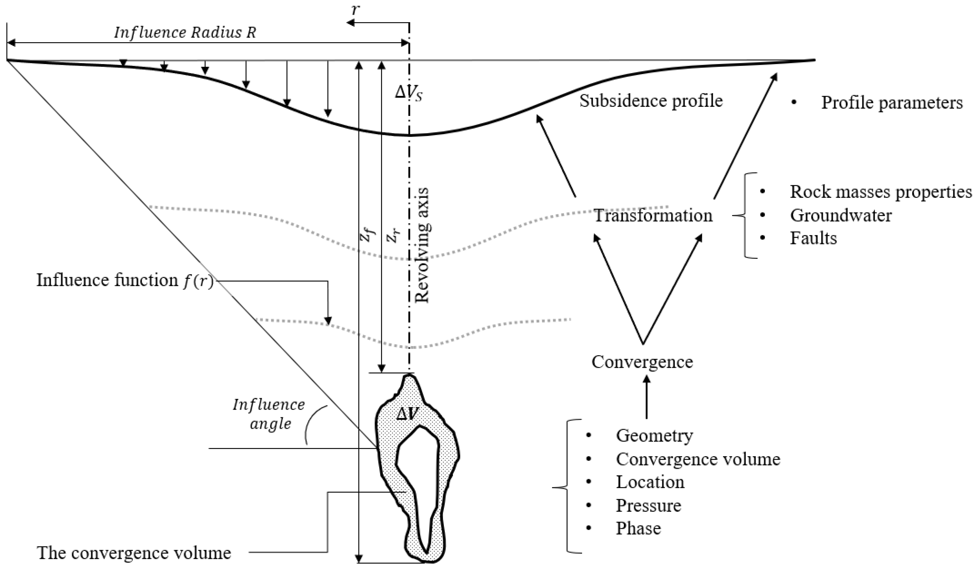
2. Ground Subsidence Prediction Models in the Context of Salt Caverns

Ground subsidence prediction is a field of subsidence engineering that uses and develops methods to describe the state of surface deformation caused by mining activities at a time. In the mid-20th century, the advent of solution mining posed a new challenge for subsidence engineering. Although the scale of mining was comparable to coal mining, there were significant differences in mining method, cavity geometry and depth, exploitation, and other factors, such as the cycles and phases of gas storage caverns due to leaching and filling processes, high geological uncertainty, and surrounding mass creep [4]. As a result, empirical ground subsidence prediction methods are used in coal mining, which are not directly applicable. Thus, predicting surface subsidence above caverns became a new topic within the subsidence engineering field [5]. Despite these differences, the general approach to solving the problem remained the same. In general, subsidence at a surface location can be calculated as the influence of underground elements using Equation (1) [6]. The values used in the equation are independent and can be synthesized in various ways.

$$S=∆V·a·e$$

(1)

where; $a$ is a transmission coefficient; $e$ is an influence factor; and $∆V$ is an underground convergence volume.

Kratzsch [6], Peng [7], and other authors classify ground subsidence prediction methods based on their methodological approaches. The solution to the subsidence prediction problem relies on estimating parameters, which can be performed by using (a) physical methods, based on a physical interpretation of the subsidence process and physical parameters, (b) empirical methods, based on statistical interpretations of the ground subsidence profile’s geometrical parameters, or (c) mixed methods, which combine empirical and physical features. Despite these differences, all the methods can be described using the factors in Equation (1), which are convergence $∆V$, transmission coefficient a, and influence factor e.

2.1. Convergence

The International Society for Rock Mechanics (ISRM) defines convergence in rock mechanics as “the time dependent closure of a fractured rock mass under compressive stress, often as a result of excavation, and usually measured perpendicular to the excavation face” [8]. Despite the definition in the subsidence engineering field, particularly for cavern fields, convergence refers to the volume change in the cavern, according to the boarders’ displacement. The meaning of transformation appeared as part of the development of subsidence prediction methods [9]. The convergence process can be described by different parameters, such as in the article regarding the convergence volume at the given time t s, which is denoted as $∆V\left(t\right)$.

In contrast to classical mining, the processes inside a cavern used for gas storage are not directly observable, therefore geomechanic models have been established. The cavern’s pressure state is dynamic during long-term operation and depends on the mining phase, the operational mode, and the physical processes occurring inside the cavern. Gas cavern storage involves periodic variations in operation, including low-pressure operation, gas injection and pressurization, high-pressure operation, and gas recovery and depressurization stages. Another complexity of estimating convergence is related to the lack of ability to continuously measure the cavern during exploitation, and, thus, this results in difficulty in defining the strain of the salt under pressure. For example, one of the complexities is related to the creep process, which is described by different models, depending on various factors, including microstructure and NaCl content in the rock mass. The general effect of these factors on the creeping process is described in

Table 1. General tendencies of salt characteristics in relation to the creeping model [10,11,12], where $\epsilon$ defines the strain.

Characteristic	Influence
Confining pressure	An increase in stress increases strain rate over time $\frac{d\epsilon }{dt}$. However, when confining pressure exceeds 4 MPa, the creep behaviour of salt rock is independent of confining pressure.
Temperature	The higher the temperature (T), the faster the creep rate. When the other conditions remain unchanged, the higher the temperature, the faster the creep rate, and, the larger the creep strain, the shorter the creep life.
NaCl content	The decay creep rate and steady creep rate of salt rock increase with the increase in NaCl content.
Water	Water can be formed nearby the grain structure, which can promote the release of elastic energy stored in salt rock and accelerate the creep development process of salt rock. In geomechanics, creep life refers to the amount of time it takes for a material to deform or fail under a constant load or stress.

.

Since many factors are influenced by salt cavern convergence, the modelling or a prediction of the convergence are complicated tasks. There are several models, which were established, to estimate the convergence at a particular time, and the models presented below are divided into groups based on solution approaches.

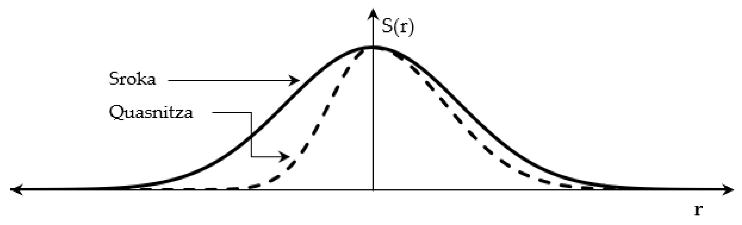
2.1.1. Convergence Models

Physical Models

Physical models, in this context, refer to using physical principles and parameters of the system in mathematical models to estimate the convergence.

Solutions according to Norton’s power law: Norton’s power law describes the strain rate of the rock masses due to the creep deformation. Van Sambeek [13] represents the long-term creep response of a cylindrical cavern based on the material law of Norton-Hoff. This is applied to calculate the convergence rate at a given time in cylindrical coordinates $z$, as well as $a_M$ (Equation (2)).

$$\frac{dV}{dt}=-\frac{3A{e}^{-\frac{Q}{R_{0}T}}{\left(\frac{\sqrt{3}}{n}·\frac{{\gamma }_{salt}-{\gamma }_{brine}}{\mu }·z\right)}^n{a}_M^2}{2r}$$

(2)

where; $a{}_M$ is a radius of cavern (m); z is depth (m), ${\gamma }_{salt} \mathrm{and} {\gamma }_{brine}$ are the stress and pressure gradients (MPa/m) for salt and brine, respectively; Q is the activation energy for salt, 12.9 kcal/mol; $R_0$ is a gas constant equal to 8.31441 kJ/(mol·K⁻¹); A is a material constant that for salt 1.313 × 10⁹, s; T is a rock mass temperature; n is a another material constant that define slope of linear approximation of $\log \left(\frac{d\epsilon }{dt}\right) of \log \left(\sigma \right)$; and $\sigma$ is stress.

The solution of Norton’s power law for the creep shrinkage volume rate of the spherical cavern can be deduced by Equation (3) [4]. The time is implicitly included in the pressure measurements. The creep shrinkage volume rate of the spherical cavern can be calculated based on these measurements. This allows for the determination of the annual volume shrinkage.

$$\frac{dV}{dt}=2a_M^{3}A\left(1-{\nu }_0\right){\left(\frac{3}{2n}\left(P_{\infty }-P_t\right)\right)}^n$$

(3)

where; ${\nu }_0$ is Poisson coefficient of the surrounded rock masses; $P_{\infty }$ is initial in situ ground stress (MPa); and $P_t$ is a gas pressure in the cavern at the time t (MPa).

Dreyer: The cavern convergence defined by Dreyer refers to the convergence of a cavern that is used for storage of natural gas, oil, or other materials. He defines the convergence rate as a function influenced by the factors rock properties, temperature, shape and size of the cavern, and the stress state of the surrounding rock mass. Dreyer approximates the physical influence of the aforementioned factors and provides a solution (Equation (4)) [6], where, for each factor, the power of the influence is estimated from data. The convergence is described by the calibration of different factors: the pressure imbalance, the temperature, and the geometry of the cavern (Equation (4)).

$$∆V\left(t\right)=V·a_D\left[1-\frac{D}{h}\left(1-\frac{D}{2h}\right)\right]{\left(\frac{P_{\infty }-P_t}{P_{ref}}\right)}^{l_D}{\left(1+\frac{\vartheta }{{\vartheta }_{ref}}\right)}^{m_D}{\left(\frac{t_{op}}{t_{ref}}\right)}^{n_D}$$

(4)

where; D is a diameter of the cavern, m; h is a high of the cavern, m; $a_D$ is a rock mass factor in the range from 0.1 to 8.12%, depending on the thickness of the overburden and the rock mass quality; ${\vartheta }_{ref}$—reference— is 273 degrees C; $\vartheta$ is the temperature in the cavern; $m_D$ is the power of the temperature influence in the range from 1.70 to 6.4, depending on the shape and size of the excavation and the geological structure of the rock mass; $P_{\infty }$ is a lithospheric pressure; $P_t$ is an actual pressure in the cavern at the given time t; $P_{ref}$—reference— is the grade (250 bar); $l_D$ is the power of pressure difference influence in the range from 1.2 to 2.95, depending on the depth of the excavation and the mechanical properties of the rock mass, such as the uniaxial compressive strength and the modulus of elasticity; $t_{op}$ is operation time, $t_{ref}$ is the reference grade of one month; and $n_D$ is the power of influence of operation time in the range from 0.32 to 0.94, depending on the level of confinement and the stress state of the rock mass.

Statistical Models

Here, the convergence model is not based on a physical law, but rather empirically inferred from observations. These can be direct or indirect. Direct observations refer to volumetric measurements of the cavern itself at different time intervals. Indirect observations relate to ground deformation monitoring, whose results are used to infer the convergence as a parameter.

Schober and Sroka [9] implement the convergence rate as part of a ground subsidence prediction method and introduce a particular parameter. Additionally, a time delay for the transmission process through the overlaying rock mass is introduced, which is the ground subsidence volume at time t ($V_s\left(t\right)$) (Equation (5)).

$$V_s\left(t\right)=aV\left(1+\frac{f}{{\xi }_S-f}\cdot \exp \left(-{\xi }_S\cdot t\right)-\frac{{\xi }_S}{{\xi }_S-f}\exp \left(-f·t\right)\right)$$

(5)

where; $a$ is a coefficient of volume losses (a = 1.0 is a passage through the rock mass without a volume loss); $V$ is an initial volume of the cavern; ${\xi }_S$ is a relative rate of volumetric convergence (e.g., ${\xi }_S$ = 0.02 year⁻¹ means that the volumetric convergence proceeds at a rate of 2% of the current volume per year); and $f$ is the relative rate of trough passage through the rock mass, which is measured in year⁻¹.

During the process of transmitting the convergence volume on the surface, some of the volume may be lost. This loss of volume leads to a discussion of the transmission coefficient, which is provided in the following chapter.

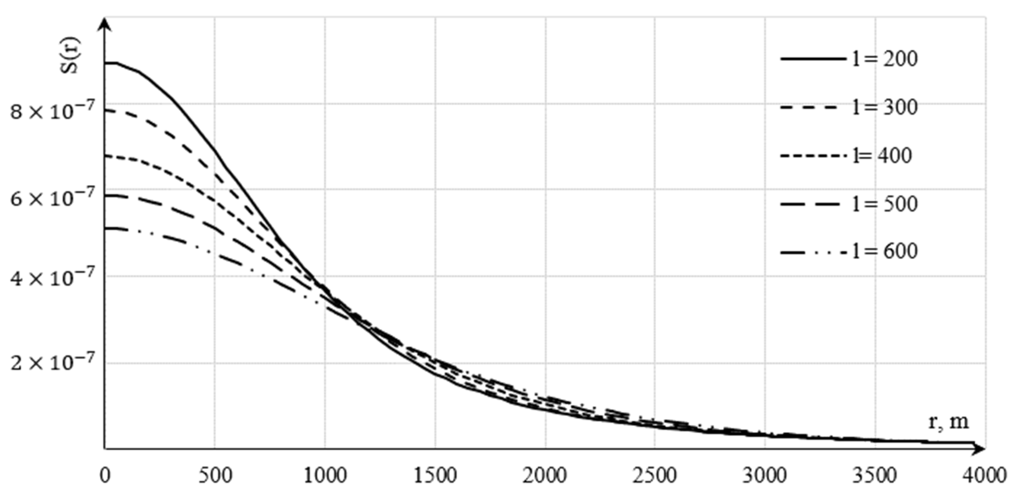
2.2. Transmission Coefficient a

The transmission coefficient is a factor that quantifies the proportion of the convergence volume that ultimately leads to the volume of ground subsidence ($V_s$) over an infinite time horizon. It can be mathematically defined by Equation (6).

$$a=\frac{V_s}{∆V}$$

(6)

The influence of the transmission coefficient and the convergence rate on the timely subsidence process can be strongly overlapping. The precise estimation of the transmission coefficient strictly can only be made in the condition of completed subsidence. In practise, the condition cannot be achieved during exploitation time and years after it. Thus, in the following contribution, the transmission coefficient is assumed to be one [14]. In the following section, the discussion, the transmission coefficient is not further considered.

2.3. Influence Factor e

The influence factor ‘e’ represents the proportion of ground subsidence at a particular location at the surface caused by a unit volume of ground subsidence or convergence beneath that point. This is affected by the distance from the point and the distribution of deformation, which is described by the influence function $f\left(r\right).$ The principle behind the influence function is the ‘volume balance’ concept, where the volume of convergence ($\Delta V$) and volume of ground subsidence $V_s$ should be equal (as shown in Equation (7)).

$$\Delta V=V_s$$

(7)

The volume of the subsidence can be determined by solving the integral beneath the surface of the influence function (Equation (8)). The solution of this equation provides a means to weigh the influence function in a way that satisfies the volume balance condition of the general prediction method (Equation (1), Figure 1).

$$\underset{0}{\overset{2\pi }{\int }}\underset{0}{\overset{\infty }{\int }}f\left(r,\phi \right)rdrd\phi =\Delta V$$

(8)

where; $\phi$ is a horizontal angle between vector r and geographical north direction.

2.3.1. Physical Methods

In subsidence engineering, a mechanical solution is used to determine the deformation by solving static equilibrium equations either analytically or numerically. Although geomechanic tasks are often solved using FEM methods, this topic is not discussed in this article, since the method is not preferred in ground subsidence prediction due to the complexity of the geological conditions and the computational resources required.

One of the earliest methods for predicting subsidence above caverns was developed by Mogi [15], who focused on the influence of underground magmatic caves. Mogi estimated the position of the magma accumulation to predict potential subsidence regions resulting from changes in magma occupancy, using the static equilibrium equation for elastic deformation. The idea of rock deformation as an elastic deformation became a basic physical model for predicting subsidence above caverns. In 2019, Ike provides the solution of the axisymmetric elasticity problems of the homogeneous, isotropic, linear elastic half-space [16].

Ike solution [16]. Later, the solution of Ike is implemented for a case of salt caverns in the form of Equation (9) [4].

$$S\left(r\right)=\frac{(1-v_o)∆V\left(t\right)}{\pi }{\int }_0^{\infty }\left(\frac{k}{1+{k^{3}l}^3}·e^{-kz}{J}_0\left(kr\right)\right)dk$$

(9)

where; $∆V\left(t\right)$ is a convergence volume at the time t; z is depth of the cavern; $l$ is a stiffness radius of the plate (Equation (10)); r is a horizontal distance between centre of a cavern and surface; $v_o$ is a Poisson ratio of the semi-infinite body; $J_0$ is a zero-order Bessel function of the first kind point; k is an integration parameter that takes a value from 0 to infinite; t is a time in years. The variable k varies from zero to infinite and disappears after integration.

$$l=\left(\frac{E{h}^3}{12\left(1-v^2\right)k_l}\right)$$

(10)

where; $E$ is the Young’s Modulus of the slab; $h$ is the thickness of the beam; $v$ is the Poisson’s ratio of the slab; and $k_l$ is the modulus of subgrade reaction.

The model separates the depth (z) and the relative location (r) in the equation. It belongs to the solution for deformation presented by Ike, where strain is divided into horizontal and vertical vectors to obtain the solution. It defines the strength of the material as the stiffness radius. The total convergence defined by material strength property. Figure 2 demonstrates the influence of the estimated strength on subsidence profile. According to the formula (a), an increase in strength of the material in overlaying rocks results in a smaller subsidence volume, and (b) a decrease in the Poisson ratio increases the subsidence volume.

2.3.2. Statistical Methods

The statistical interpretation relates to the approximation of a subsidence profile as a spatial distribution of the mined volume on the surface. It is supposed to be distributed around geometrical centre of the void. The distribution is described by an influence function. In this context, there are several approaches documented.

Sroka and Schober. The method introduced by Sroka and Schober (Equation (11)) [9] uses a Gaussian function to describe the spatial subsidence distribution. Ground observations, e.g., from geometric levelling, are used to estimate the parameters of this influence function. It excludes any physical characteristic and can be used as good prototype for further connection of physical processes.

$$S\left(r,t\right)\cong \frac{∆V\left(t\right)}{R^2}\exp \left(-\frac{\pi r^2}{R^2}\right)$$

(11)

where; R is a radius of maximum influence and is defined as $R=\sqrt{{z_{f}z}_r{\cot }^2\beta }$; $\beta$ is the so-called angle of main influences. Later, ref. [14] suggested some adjustment of the influence radius of roof by adding influence of the cavern roof characteristic c and surface factor n as $R_r\left(z\right)=R{\left(\frac{z-z_r+c}{z_r-z_f+c}\right)}^n$.

Eickemeier’s approach is formulated in Equation (12), where the power ($\delta$) of the relative position ($\frac{r}{R}$) defines the shape and, thus, the inclination of the subsidence trough wings [16]. The difficulty related to this solution is in finding the integral of the volume under the rotated function because there are no analytical solutions available for arbitrary parameters $\delta$.

$$S\left(t,r\right)=-\frac{\xi \delta }{2{\pi }^{1-\frac{2}{\delta }}{R}^2\Gamma \left(\frac{2}{\delta }\right)}\exp \left(-\pi {\xi }^{\frac{\delta }{2}}\frac{r^{\delta }}{R^{\delta }}\right)·V_{conv}\left(t\right)$$

(12)

where; $\xi$ is called by the author “a parameter to consider a time effect”. In praxis, it should be used for a fine calibration of the maximum subsidence; $\delta$ is a form parameter that describes a change in the curvature of the influence function (range from 1.5 to 3); $\Gamma$ is a gamma function that normalizes the function with respect to the convergence volume. The effect of the variables on the subsidence can be seen in Figure 3.

The difficult part of the solution is the consideration of the volume balance and variety of the definition of the influence radius. This creates problems to use $\delta$ as a parameter that is to be estimated from observations.

Quasnitza proposed a mathematical solution to describe an asymmetrical shape of the subsidence trough (Equation (13)) [17]. For this propose, R is presented as a function of horizontal angle $\phi$ between profile line and the geodetic north direction. The volume of the shape depends on the function $R\left(\phi \right)$. The distribution is provided in Figure 4.

$$S\left(r,\phi \right)=\frac{a∆V}{z_r{z}_f·ctg{\gamma }_{max}·ctg{\gamma }_{min}}{e}^{-\frac{\pi r^2}{R^2\left(\phi \right)}}$$

(13)

where; ${\gamma }_{max}$ and ${\gamma }_{min}$ are influence angels in the direction of asymmetry (in the context of the influence radius shown in Figure 5); $z_r{ \mathrm{and} z}_f$ denotate the depth of the roof and floor of the cavern, respectively.

As a demonstration, a synthetic example based on an asymmetric function $R\left(\phi \right)=R+\frac{1}{3}R\ast \cos (\phi (X,r)+\frac{1}{3}\pi )$ is shown in Figure 4, Figure 5 and Figure 6. The distribution of R is provided in Figure 5 in profile Y = 0, as well as in Figure 6, in three dimensions. Another factor to consider is that the Quasnitza solution does not appropriately account for convergence volume, which is addressed and corrected in the related chapter.

2.4. Conclusions

There are two types of models used to describe the convergence behaviour of caverns: physical models and statistical models. However, empirical models are more often used in practice due to the need for a sufficient amount of sample data to estimate physical parameters. In the specific case of caverns used for storage, it is crucial to include pressure data in the convergence part of the subsidence equation.

Regarding the influence function, the Gaussian distribution is considered the basic subsidence shape. However, Eickemeier suggests that the shape of the distribution can vary and introduces additional shape parameters. Quasnitza extends Sroka’s approach to cover asymmetry, but the original approach requires an adjustment to consider volume balance. As the need to cover asymmetrical subsidence shapes was identified [18], the correction of the Quasnitza solution is discussed, including the generalization of bivariate limits.

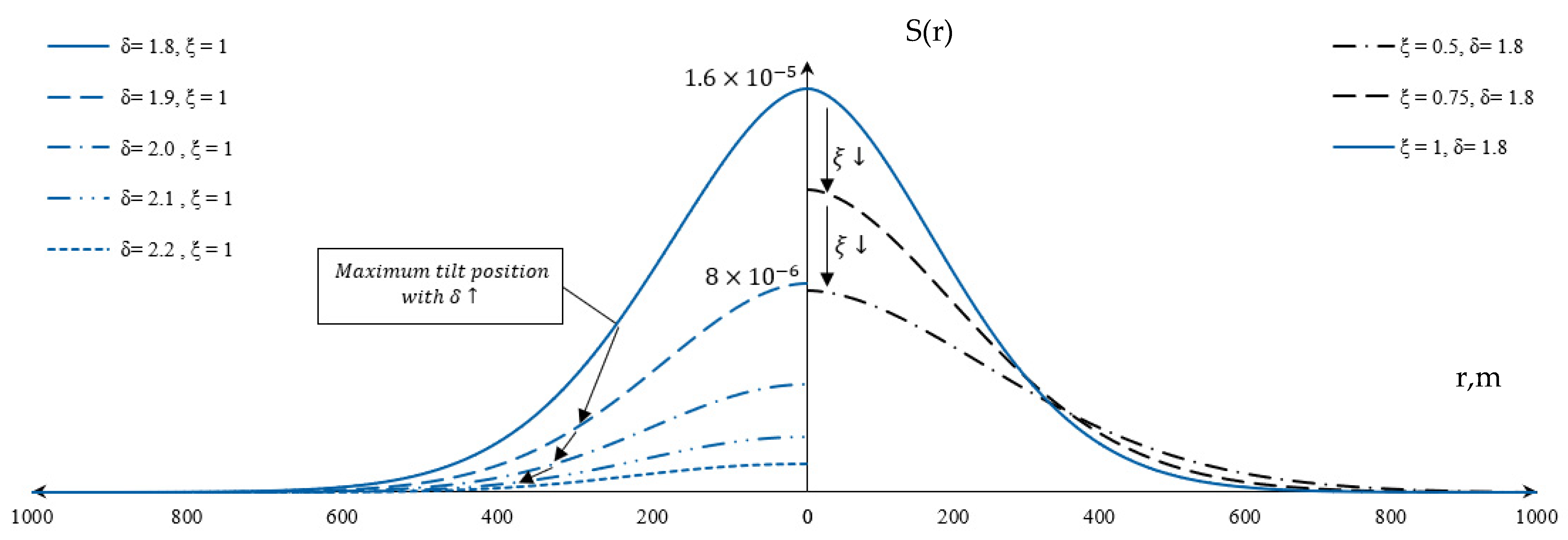
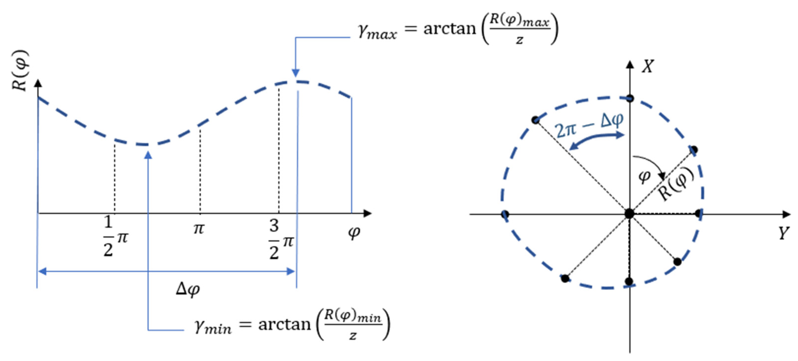
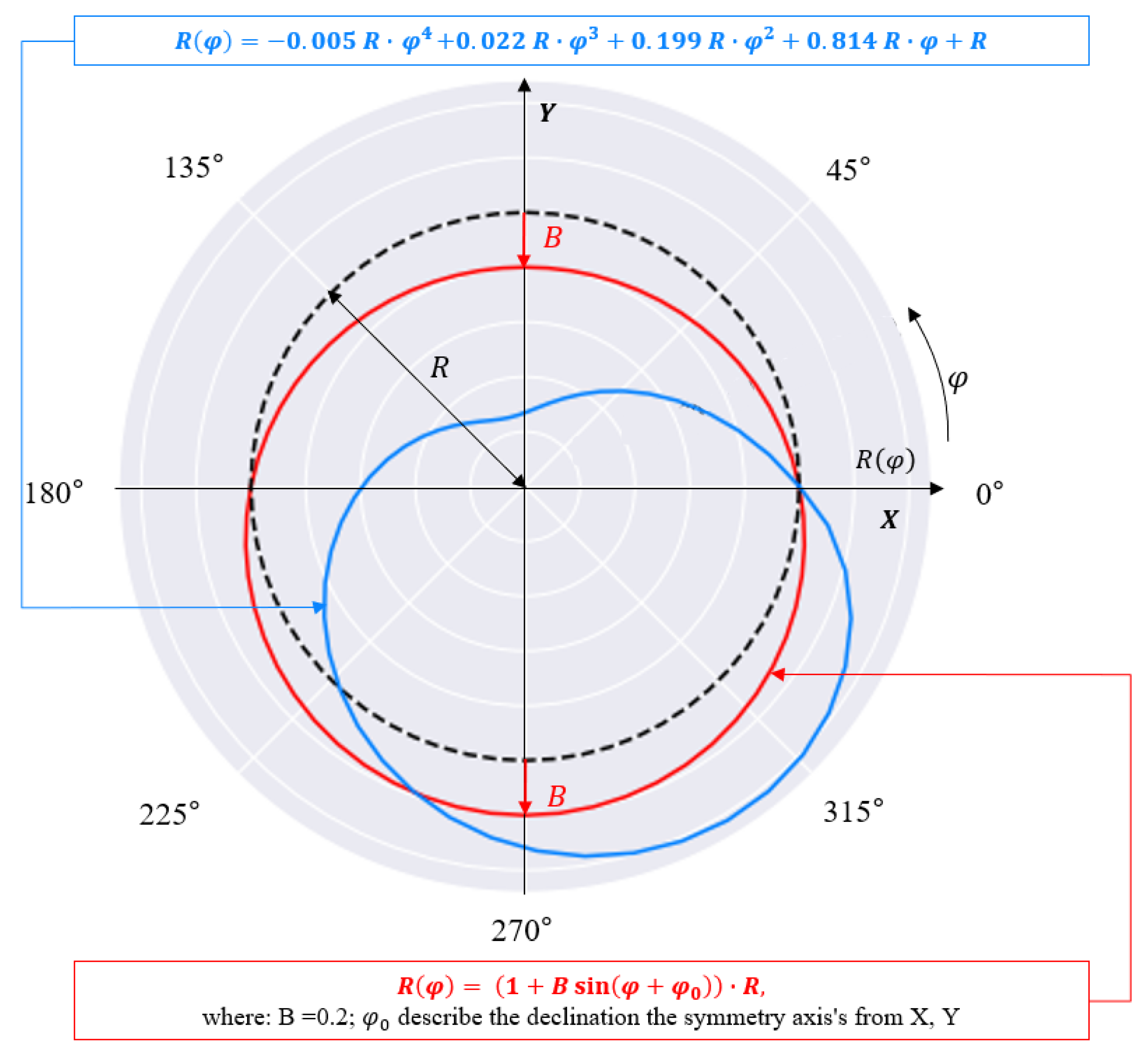
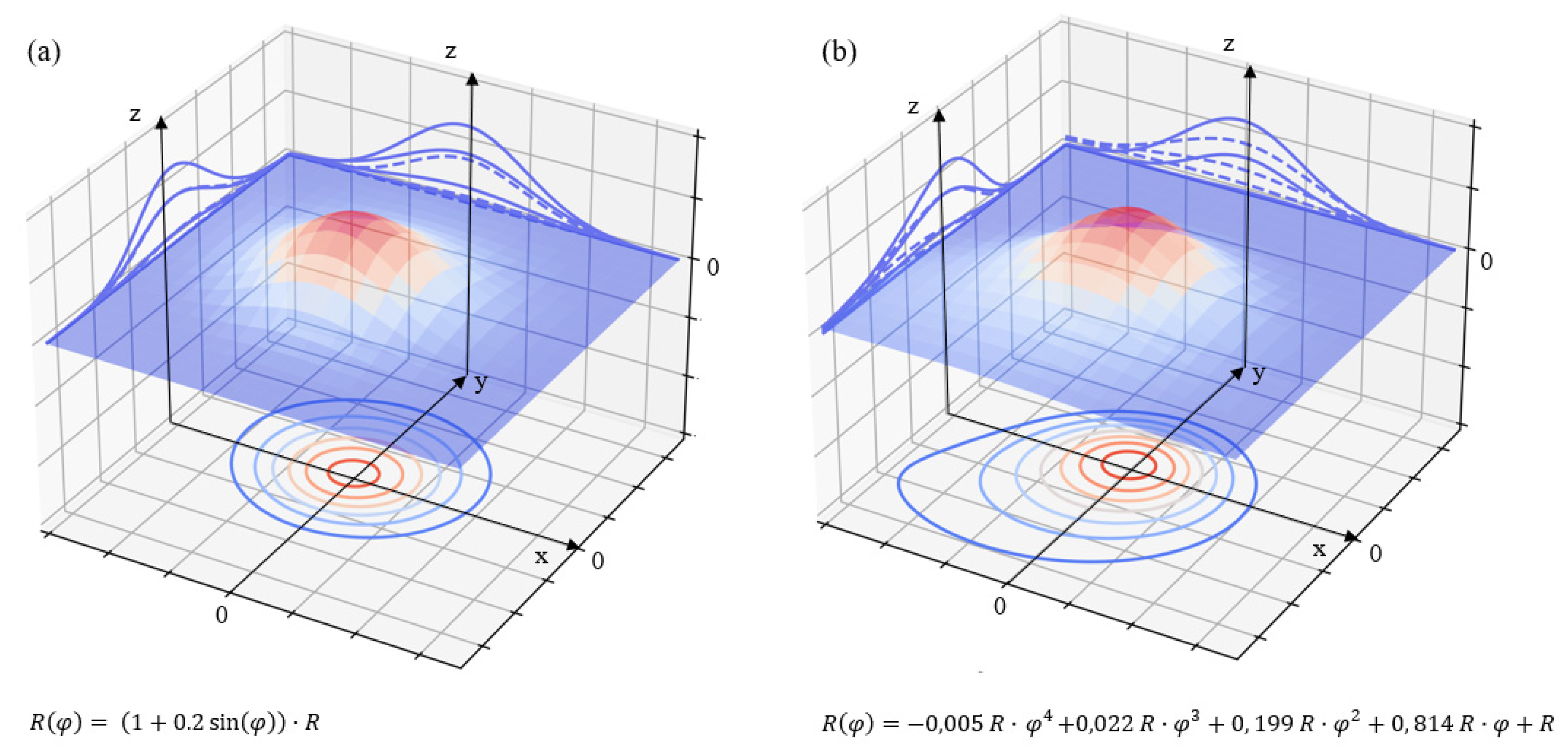
3. Introducing Asymmetry in the Model

Around the world, numerous instances of asymmetrical subsidence are being observed, often associated with stress-related factors [18]. For instance, asymmetric subsidence and the formation of subsidence bowl shapes have been documented in various countries, such as Sweden [19], the USA [20], Canada [21], Ghana [22], China [23,24], among others. These examples emphasize the considerable potential for mathematically correcting the asymmetrical extensions and developing a generalized approach for predicting ground subsidence that can effectively account for asymmetry.

The influence function is a crucial component of subsidence prediction models, as it describes the spatial distribution of subsidence and how it varies with distance from the cavern. The function is regulated by the influence radius R, which is defined in Equation (14).

$$R=z cot \left(\gamma \right)$$

(14)

where; $z$ is a depth of the cavern; $\gamma$ is an influence angle.

To simplify matters, this paper utilizes the term “influence radius”, as it is proportional to the influence angle and depth. However, in practical applications, estimating the influence angle is more significant, since the depth of caverns may differ. To introduce asymmetry, the influence function should be direction-dependent. The direction is defined as the angle φ in Equation (15), which is the horizontal angle between vector r and the North direction on the X–Y axis.

$$\phi =arcctg\left(\frac{∆y}{∆x}\right)$$

(15)

To express the asymmetry of the subsidence bowl, a continuous function should be implemented in R that depends on 𝜑 and is defined between 0 and 2π to describe a closed contour. In the symmetric case, $R\left(\phi \right)$ is described as a constant with a constant value. For each specific asymmetrical case, it is important to meet the requirement of volume balance between the convergence volume and subsidence volume. Therefore, the solution of Equation (9) takes the shape shown in Equation (16).

$$\underset{0}{\overset{2\pi }{\int }}\underset{0}{\overset{\infty }{\int }}\exp \left(-\mathsf{\pi }\frac{{\mathrm{r}}^2}{{R\left(\phi \right)}^2}\right)r dr d\phi =\underset{0}{\overset{2\pi }{\int }}\frac{{R\left(\phi \right)}^2}{2\pi }d\phi =\frac{1}{2\pi }\underset{0}{\overset{2\pi }{\int }}{R\left(\phi \right)}^{2}d\phi$$

(16)

The value of $R\left(\phi \right)$ can be defined by any equation meeting the above-mentioned requirements. Examples of such functions are provided in Equations (17) and (18) and illustrated in Figure 7 and Figure 8. These examples use trigonometric and polynomic function.

$$R\left(\phi \right)=\left(1+B\sin \left(\phi \right)+\Delta \mathsf{\phi }\right)·R$$

(17)

$$R\left(\phi \right)=-0.005R·{\phi }^4+0.022R·{\phi }^3+0.199R·{\phi }^2+0.814R·\phi +R$$

(18)

where; R is some average meaning of the influence radius estimated by influence angle for several directions. Δφ is an angle from the North direction to state the direction of asymmetry. In the example, Δφ is assumed to be 0.

In both cases (using either a trigonometric function or a polynomial function), it is important to estimate the influence angle in order to obtain the property of influence radius:

• For the trigonometric function, the influence angle should be estimated either in the two directions of asymmetry: Δφ and Δφ + 1/2 π, or if they are unknown (usually) in three directions. Alternatively, the difference in direction should be concluded beforehand. In the case, R represents an average of $z·ctg\left(\gamma \right)$ in these two directions.
• For the polynomial function, the influence angle should be estimated in five different directions in order to estimate the polynomial function. The value of R in this case is the same, as in the sin function case, i.e., an average of $z·ctg\left(\gamma \right)$.

To calibrate the new function according to Equation (8), Equation (16) must be solved. In the case of R(φ) being defined as a function by Equation (17) or Equation (18), an analytical solution is provided in Equations (19) and (20), respectively. Both models are presented in Figure 7.

$$\begin{array}{r}S\left(r,\phi \right)=\frac{\Delta V}{\frac{1}{2\pi }{\int }_0^{2\pi }{\left(R+RBsin\left(\phi \right)\right)}^{2}d\phi }·\exp \left(-\frac{\pi r^2}{R{\left(\phi \right)}^2}\right)=\\ \frac{\Delta V}{\frac{1}{2}{R}^2\left(2+B^2\right)}·\exp \left(-\frac{\pi r^2}{R{\left(\phi \right)}^2}\right) \end{array}$$

(19)

$$\begin{array}{r}S\left(r,\phi \right)=\dots =\frac{\Delta V}{\frac{1}{2\pi }{\int }_0^{2\pi }{R\left(\phi \right)}^{2}d\phi }·\exp \left(-\frac{\pi r^2}{{\left(R\left(\phi \right)\right)}^2}\right)=\\ =\frac{2\pi \Delta V}{96.5229R^2}·\exp \left(-\frac{\pi r^2}{{\left(R\left(\phi \right)\right)}^2}\right) \end{array}$$

(20)

The demonstration of the aforementioned definition for $R\left(\phi \right)$ in Equation (19) (Figure 7) is provided in Figure 8a. The demonstration of the aforementioned definition for $R\left(\phi \right)$ in Equation (20) (Figure 7) is provided in Figure 8b.

The presented example demonstrates that the asymmetry of the subsidence trough can be described if the distribution of R or $\gamma$ is known. However, in practice, the value of R is estimated from subsidence measurements. Thus, the complexity of the subsidence trough in terms of the parameters number is limited by the availability of reliable measurement points and computational power (due to operation of the matrix transforming), as solving an equation with n unknown parameters requires n + 1 statistically independent data points. Pre-estimation of the shape of the trough as a simple figure with one asymmetrical direction, such as a sine function, an ellipsoid, etc., can be applied in cases of anisotropic uniformly distributed horizontal stress, simple anisotropies, geological structures, significant changes in the landscape, etc. Some of the aspects of this topic have been investigated in the research of tectonic stress influence on the subsidence profile parameters [17], they are beyond the scope of this study.

4. Conclusions

Since salt caverns are used for storing natural gas and liquids, subsidence prediction methods must be adapted to the unique conditions of salt cavern exploitation. In general, this research provides a deep understanding of the factors involved in subsidence prediction and estimates standards and directions for quality development. It emphasizes that the solution should be chosen for each particular case, depending on the availability of data and the potential for parameter estimation. The potential of subsidence prediction lies in the unifying solution that encompasses deviations from normal distribution and defines convergence, especially in relation to the time function. The study primarily focuses on two aspects: convergence and asymmetry of the influence function, with a particular emphasis on correcting the asymmetrical extension proposed by Quasnitza.

The suggested method extends the coverage to include any type of asymmetry, in contrast to the originally proposed unilateral asymmetry and corrects the mathematical aspects of the original solution to ensure volume equilibrium. Therefore, the article ex-tends theoretical bases on the ground that subsidence prediction methods for asymmetrical cases are presented.

As an outlook of the study, the implementation of head pressure in the convergence estimation models and the estimation of the necessity of shape deviation from Gaussian can be considered.

References

1. Crotogino, F. Traditional bulk energy storage—Coal and underground natural gas and oil storage. In Storing Energy, 2nd ed.; Elsevier: Amsterdam, The Netherlands, 2022; pp. 831–847. ISBN 9780128245101. [Google Scholar] [CrossRef]
2. Wolf, E. Electrochemical Energy Storage for Renewable Sources and Grid Balancing; Elsevier: Amsterdam, The Netherlands, 2015. [Google Scholar]
3. Warnecke, M.; Röhling, S. Untertägige Speicherung von Wasserstoff—Status quo. Z. Dt. Ges. Geowiss. 2021, 172, 641–659. [Google Scholar]
4. Ye, L.; Chen, F.; Ma, H.; Shi, X.; Li, H.; Yang, C. Subsidence above rock salt caverns predicted with elastic plate theory. Environ. Earth Sci. 2022, 81, 123. [Google Scholar] [CrossRef]
5. Del Greco, O.; Garbarino, E.; Oggeri, C. A Multidisciplinary Approach for the Evaluation of the “Bottegone” Subsidence (Grosseto, Italy). In Engineering Geology for Infrastructure Planning in Europe; Hack, R., Azzam, R., Charlier, R., Eds.; Lecture Notes in Earth Sciences; Springer: Berlin/Heidelberg, Germany, 2004; Volume 104. [Google Scholar] [CrossRef]
6. Kratzch, H. Bergschadenkunde; Deutscher Markscheider-Verein e. V.: Bochum, Germany, 2013. [Google Scholar]
7. Peng, A. Surface Subsidence Engineering: Theory and Practice; CRC Press: Boca Raton, FL, USA, 2020. [Google Scholar]
8. Ulusay, R. The ISRM Suggested Methods for Rock Characterization, Testing and Monitoring: 2007–2014; Springer International Publishing: Berlin/Heidelberg, Germany, 2015. [Google Scholar]
9. Sroka, A.; Schober, F. Die Berechnung der maximalen Bodenbewegungen über kavernenartigen Hohlräumen unter Berücksichtigung der Hohlraumgeometrie. Kali U. Steinsalz 1982, 8, 273–277. [Google Scholar]
10. Hunsche, U.; Hampel, A. Rock Salt—The Mechanical Properties of the Host Rock Material for a Radioactive Waste Repository. Eng. Geol. 1999, 52, 307–321. [Google Scholar] [CrossRef]
11. Zhang, Q.; Song, Z.; Wang, J.; Zhang, Y.; Wang, T. Creep Properties and Constitutive Model of Salt Rock. Adv. Civ. Eng. 2021, 2021, 8867673. [Google Scholar] [CrossRef]
12. Holdsworth, S. Constitutive Equations for Creep Curves and Predicting Service Life. In Creep-Resistant Steels; Woodhead Publishing Series in Metals and Surface Engineering; Woodhead Publishing: Sawston, UK, 2008; pp. 403–420. ISBN 9781845691783. [Google Scholar] [CrossRef]
13. Van Sambeek, L. Evaluating Cavern Tests and Surface Subsidence Using Simple Numerical Models. In Proceedings of the Seventh Symposium on Salt, Kyoto, Japan, January 1992; Volume I, pp. 433–439. [Google Scholar]
14. Tajduś, K.; Sroka, A.; Misa, R.; Tajduś, A.; Meyer, S. Surface Deformations Caused by the Convergence of Large Underground Gas Storage Facilities. Energies 2021, 14, 402. [Google Scholar] [CrossRef]
15. Mogi, K. Relations between the Eruptions of Various Volcanoes and the Deformations of the Ground Surfaces around Them. Bull. Earthq. Res. Inst. 1958, 36, 99–134. [Google Scholar]
16. Eickemeier, R. Senkungsprognosen über Kavernenfeldern—Ein Neues Modell-.34; Geomechanik-Kolloquium: Leipzig, Germany, 2005. [Google Scholar]
17. Quasnitza, H. Eine Strategie zur Kallibrierung Markscheiderischer Bewegungsmodelle und zur Prädiktion von Bewegungselementen. Doctoral Dissertation, Technical University Clausthal, Lower Saxony, Germany, 1988. (In German). [Google Scholar]
18. Babaryka, A.; Benndorf, J. Investigation about the Contribution of Tectonic Conditions to Mining Subsidence Parameters. Min. Sci. 2022, 29, 105–118. [Google Scholar] [CrossRef]
19. Jones, T.; Nordlund, E.; Wettainen, T. Mining-Induced Deformation in the Malmberget Mine. Rock Mech. Rock Eng. 2019, 52, 1903–1916. [Google Scholar] [CrossRef] [Green Version]
20. Favorito, D.A.; Seedorff, E. Laramide Uplift near the Ray and Resolution Porphyry Copper Deposits, Southeastern Arizona: Insights into Regional Shortening Style, Magnitude of Uplift, and Implications for Exploration. Econ. Geol. 2020, 115, 153–175. [Google Scholar] [CrossRef]
21. Sepehri, M.; Apel, D.; Hall, R. Prediction of mining-induced surface subsidence and ground movements at a Canadian diamond mine using an elastoplastic finite element model. Int. J. Rock Mech. Min. Sci. 2017, 100, 73–82. [Google Scholar] [CrossRef]
22. Magambo, I.; Dikgang, J.; Gelo, D.; Tregenna, F. Environmental and Technical Efficiency in Large Gold Mines in Developing Countries. University of Johannesburg. 2021. Available online: https://mpra.ub.uni-muenchen.de/108235/ (accessed on 6 March 2023).
23. Khanal, M.; Qu, Q.; Zhu, Y.; Xie, J.; Zhu, W.; Hou, T.; Song, S. Characterization of Overburden Deformation and Subsidence Behavior in a Kilometer Deep Longwall Mine. Minerals 2022, 12, 543. [Google Scholar] [CrossRef]
24. Xia, K.; Chen, C.; Liu, X.; Fu, H.; Pan, Y.; Deng, Y. Mining-induced ground movement in tectonic stress metal mines: A case study. Bull. Eng. Geol. Environ. 2016, 75, 1089–1115. [Google Scholar] [CrossRef]
Figure 1. Ground subsidence above salt cavern, where z r and z f are depths of a roof and a floor of the cavern;  V is convergence volume;  Vs is subsidence volume; r is a horizontal distance between centre of a cavern and surface. Similar to convergence, there are physical and empirical methods to define an influence factor.
Mining 03 00020 g001
Figure 2. Calculated ground subsidence influence profile, with input data z = 1000 m and ∆V = 1, which is calculated according different subsidence profiles and relative convergence.
Mining 03 00020 g002
Figure 3. Demonstration of the influence of ξ and δ parameters on the influence function by Eickemeier.
Mining 03 00020 g003
Figure 4. Demonstration of Quasnitza’s influence function and Sroka’s on a synthetic example, where R φ = R + 1 3 R cos ( φ ( X , r ) + 1 3 π ) .
Mining 03 00020 g004
Figure 5. Sketch of the R φ function on the X–Y axis.
Mining 03 00020 g005
Figure 6. Demonstration of Quasnitza’s influence function on a synthetic example in three dimensions, where R φ = R + 1 3 R cos ( φ ( X , r ) + 1 3 π ) .
Mining 03 00020 g006
Figure 7. Definition of R φ as a function and discrete relative to the mean value.
Mining 03 00020 g007
Figure 8. Subsidence trough with asymmetry on example of the radius distribution demonstrated in Figure 7. (a) demonstrates the sinus-based distribution. (b) polynomial-based distribution.
Mining 03 00020 g008