Article

Monitoring Horizontal and Vertical Components of SAMARCO Mine Dikes Deformations by DInSAR-SBAS Using TerraSAR-X and Sentinel-1 Data

1
National Institute for Space Research (INPE), São José dos Campos, São Paulo 12227-010, Brazil
2
Sarmap S.A., Via Stazione 52, 6987 Caslano, Switzerland
*
Author to whom correspondence should be addressed.
Mining 2022, 2(4), 725-745; https://doi.org/10.3390/mining2040040
Submission received: 19 August 2022 / Revised: 28 October 2022 / Accepted: 31 October 2022 / Published: 10 November 2022

Abstract

:
This article presents an investigation of ground movement measurements based on a combination of TerraSAR-X and Sentinel-1 data, in opposite tracks, aiming to detect ground de-formation of the remaining dikes of Germano mine, after the Fundão dam collapse. The differential interferometry technique SBAS (Small Baseline Subset) was applied to obtain the deformation of the surface in different Line of Sight (LoS), in order to carry out the vector decomposition and generate the deformation measurements in the vertical and horizontal directions. A set of 37 single-look complex (SLC) images of TerraSAR-X (TSX), acquired during the period from 19 February 2016 to 15 May 2017, and 37 SLC images of Sentinel-1, acquired from 8 February 2016 to 15 May 2017, were used to perform this investigation. For the TerraSAR-X interferometric processing, a coherence threshold of 40%, 4 looks in range and 2 looks in azimuth, 1200 m of atmospheric filter, and 10 % of max normal baseline of the critical were used. For the Sentinel-1 interferometric processing a coherence threshold of 26%, 8 looks in range and 2 looks in azimuth, 1200 m of atmospheric filter, and 20% of the of max normal baseline of the critical were used. For both sensors a digital elevation model generated by Pleiades 1-A was used for removing the topographic phase component. The final results were consistent with the topographic in situ measurements, providing key information to make crucial decisions regarding risks, or even mitigation, repairs or emergency response, as well as for a better understanding of the on-going instability phenomena affecting the dikes and dams.

Graphical Abstract

1. Introduction

Currently, mining is one of the main economic activities in Brazil, which produces and exports more than 50 types of minerals. Among these, iron ore is the most prominent in the country, with Brazil being the second largest exporter of iron ore in the world market in 2020, producing 400 million metric tons of iron ore.
In turn, the activities of an iron mining company can be basically divided into the mining process, the extraction of iron ore from its place of origin, and the ore beneficiation process, which is characterized by chemical and physical operations aimed at ore treatment so that it achieves the desired commercial characteristics. Both process-es, however, generate unwanted waste.
During the mining process, materials that do not possess the desired physico-chemical characteristics are called sterile. Tailings result from processing, since the final product obtained represents only a portion of all the material extracted, and this is stored in tailings dams as the final destination of these residues.
According to the Brazilian National Mining Agency (ANM), there were 769 tailings dams identified in Brazil at the beginning of 2019, with an accumulation of 3.5 billion m3 of mining waste, and 84 tailing dams were raised using the upstream method [1]. This method is the cheapest but the least resilient of all construction types, due to the fact that water is the primary instability agent [2].
The most frequent causes of failures are overtopping and overflows, slope foundation problems including slope settlement and instability, internal erosion and infiltration, the materials used in construction and inadequate maintenance [3]. Slope failures occur in a wide range of conditions and environments and the precursor signs before a failure may not be evident.
Different procedures for monitoring tailings dams’ stability have been applied using different geotechnical instruments such as total station, piezometers, strain gauges, shape array accelerometers, inclinometers, water level indicators, and ground radars, etc. [4], providing real-time data from fast movements (mm/day to a few tens of cm/day) to very slow movements (mm/month to mm/year). Despite the accuracy and reliability of the data provided by these instruments, many precursor signals of the failures cannot be detected due to several factors, such as field measurements restricted to points or sectors of the structure, field work that can be expensive and time consuming, adverse weather conditions, accessibility restrictions, inadequate instrument field of view, and economic restrictions, etc. With the advent of differential interferometric synthetic aperture radar (A-DInSAR) technologies [5], it was possible to perform surface displacement measurements with data from radar satellites, with individual measurements’ precision better than 5 mm depending on the radar system, without field work or ground equipment, providing a dense measurement grid and synoptic view of the area of interest [5,6,7,8]. Many studies have obtained relevant results using the A-DInSAR to monitor the displacement of open pit mines [8,9,10,11,12,13,14,15,16,17,18,19,20,21,22,23] as well as underground mines [24,25,26,27,28,29,30,31].
Near Mariana city, in Minas Gerais State (southeast of Brazil) there is an iron mine complex called Germano, in which, on the afternoon of 5 November 2015, one tailings dam (Fundão dam) collapsed, and 32.6 million cubic meters of mining waste material spilled from the dam and caused the Bento Rodrigues village to be totally flooded by mudslides, with human losses and great environmental impact [3].
The most likely cause of Fundão dam collapse was due to liquefaction of the sandy tailings of the base of the dam, impairing its mechanical strength [3]. A set chain of events and conditions related to the dam construction and operations caused the collapse, such as: the original starter dike became damaged due to the increased saturation, the slimes were deposited in areas not planned, the dam rose over the slimes due to the structural problems with a concrete pipe, and a series of three small seismic shocks that happened 90 min before the collapse [32]. After the dam col-lapse, the mudflow reached the Gualaxo and Doce River, and traversed 600 kilometers before spilling into the Atlantic Ocean on the north coast of Espírito Santo state, causing huge environmental damage due to the mud plume’s effects on marine life [33,34]. Germano iron mining complex is owned and operated by SAMARCO Mineração S.A., that is a joint venture between and the Brazilian Vale S.A. and the Australian–British BHP Billiton Brazil Ltd.
Some studies using different DInSAR techniques were carried out with the objective of detecting the stability of the dam of the Germano iron mining complex, using data from TerraSAR or Sentinel-1 [14,17,18,20] satellites. The results of the measurements were obtained in the line of sight (LoS) of the satellite, which allowed for estimating for the estimation of the vertical deformation projected in the LoS, but the deformations in the horizontal direction could not be estimated with the data in a single view.
The use of radar data on opposing acquisition geometries (ascending and descending orbits) can provide more accurate measurements of vertical and horizontal displacements, using data from the same satellite for this procedure. In turn, the possibility of combining interferometric data from different sensors to perform the vertical and horizontal vector decomposition is feasible, since open access data can be used to compose both geometries. With the open access availability of data from the Sentinel-1 SAR mission, with systematic and regular survey, and its ability to perform interferometric processing [35,36,37,38,39], it is interesting as a complementary source with other radar satellites such as Cosmo-Skymed and TerraSAR, etc.
In this work, the results and the evaluation of the combination of TerraSAR-X and Sentinel-1 data are presented and discussed, in opposite tracks, aiming to detect horizontal and vertical components of the ground deformation of the remaining dikes of the Germano mine, after the Fundão dam collapse, as a novelty. The SBAS technique (small baseline subset) was used to obtain the deformation of the surface in different LoS, in order to carry out the vector decomposition and generate the deformation measurements in the vertical and horizontal directions.

2. Materials and Methods
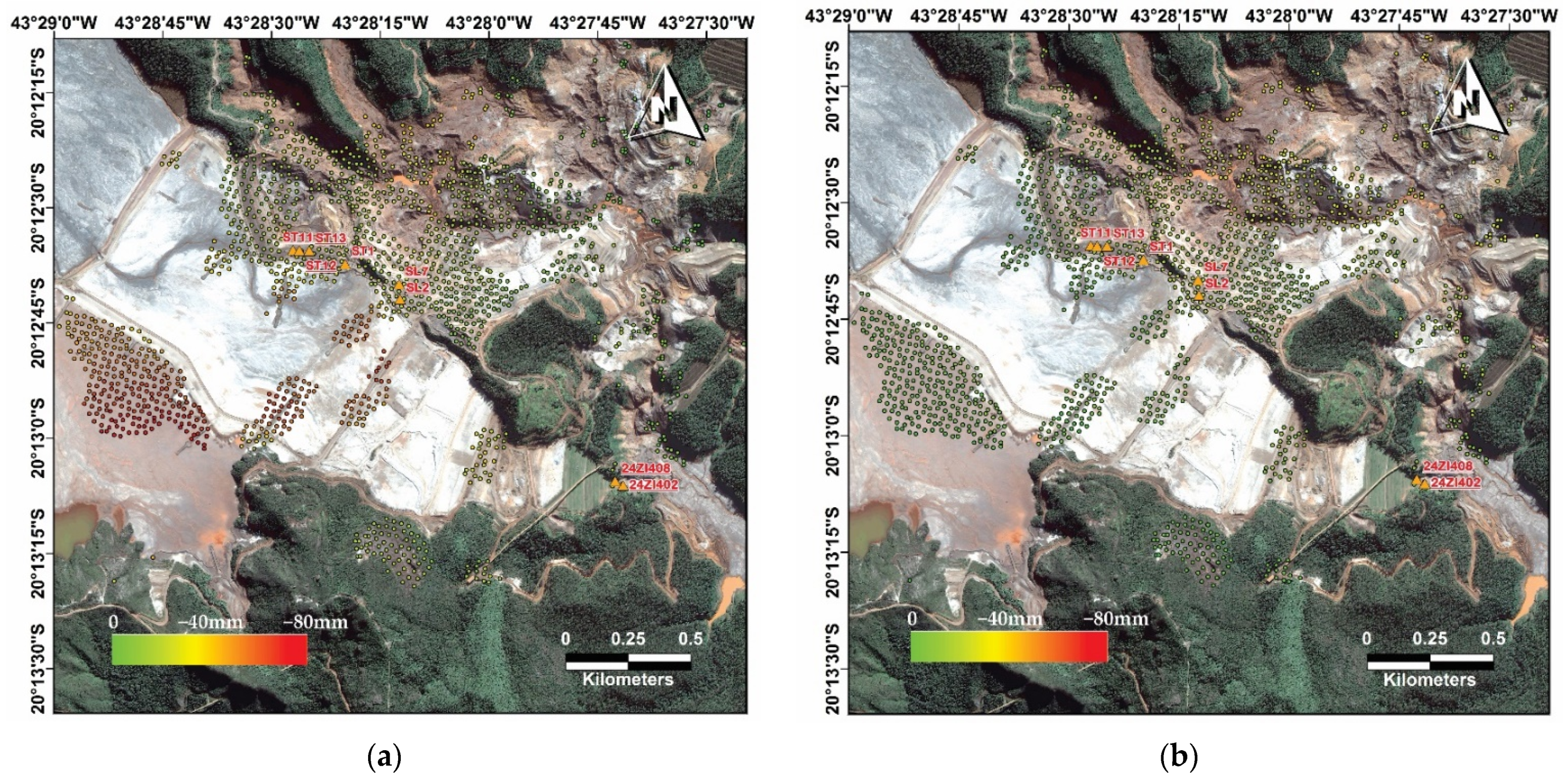
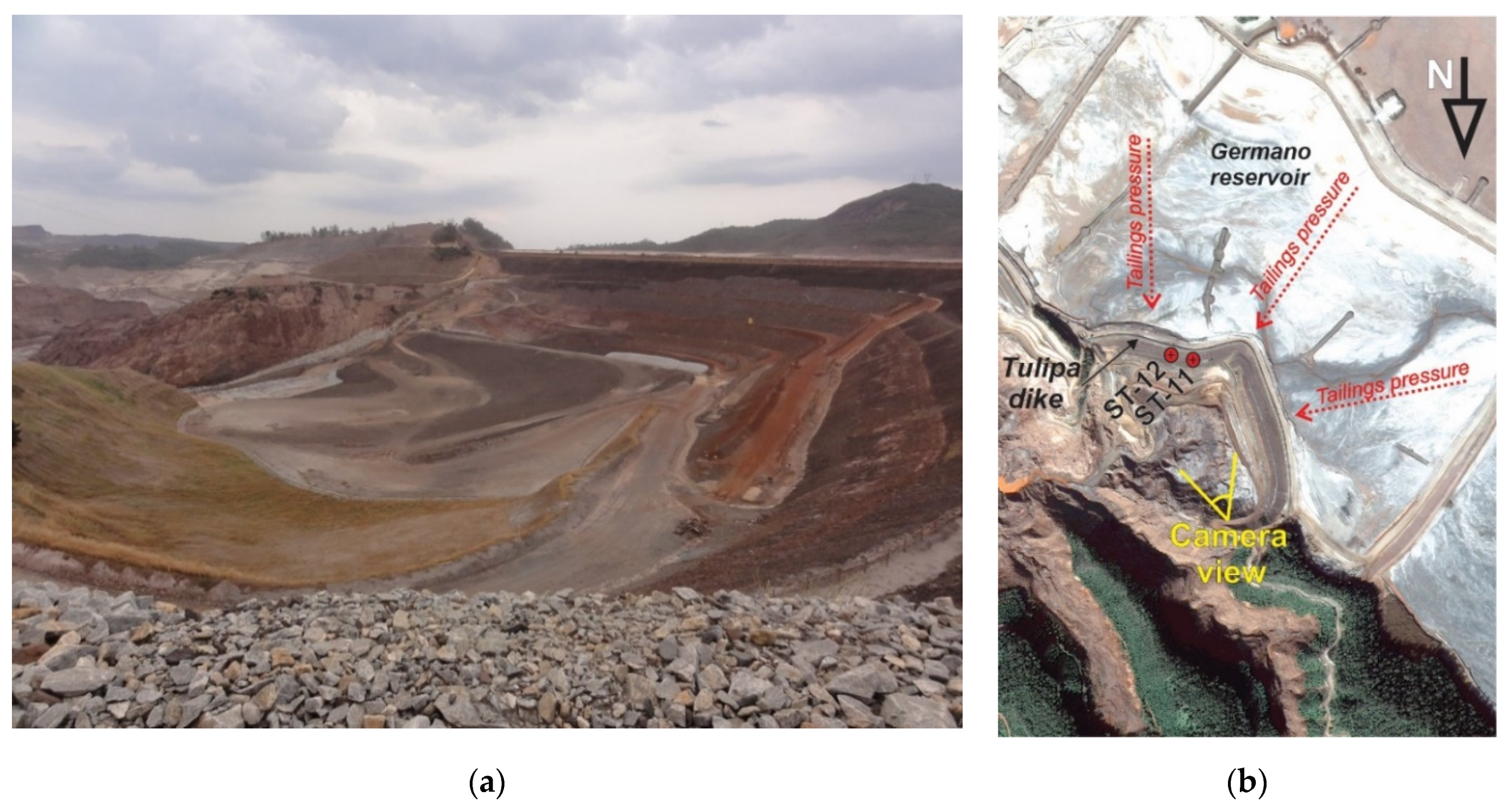
In this section, we describe the test site and the methodological approach used in this paper. This approach consists of SBAS processing and validation.

2.1. Study Area

Our experiment was performed in the Germano Iron Complex, which is located in the southern border of the São Francisco Craton, easternmost portion of the Iron Quadrangle (Quadrilátero Ferrífero—QF). This area is characterized by hilly to mountainous reliefs, diversified vegetation cover, intense anthropogenic activity (rural and urban) and mineral exploration by open pit iron mines, some already in the process of deactivation. The QF is located in the southern portion of the São Francisco Craton [40]. This geotectonic unit comprises a cratonic core stabilized in the Lower Proterozoic. Folding bands, generated in the Brasiliano cycle, limit and define the current contour of the São Francisco Craton. The QF constitutes part of the craton basement and can be characterized as follows: Metamorphic complexes; Archean volcano-sedimentary sequences of the “greenstone belt” type encompassed in the Rio das Velhas Supergroup; and platform sedimentary covers of Paleoproterozoic ages represented by the Minas Supergroup and Itacolomi Group [41].
Currently, the Germano Iron Complex is explored by the Brazilian SAMARCO Mineração S.A., with open pit mines, waste piles, industrial plants, pipelines, and tailings dams. The first tailings dam was Germano, which was installed in 1976 using the upstream method of construction with the implantation of a start dike with 70 m height. Upstream tailings dams are built progressively “upstream” of the starter dam by incorporating tailings materials into the dam for support through the controlled deposition. While using tailings materials to build the dam reduces construction costs, upstream tailings dams are more susceptible to cracking, liquefaction and erosion. This type of construction tends to be less stable than other dam design in the occurrence of seismic events, because tailings materials may liquefy and lose their strength.
This iron mining complex is an important iron producer in Brazil, and it was composed of two huge tailings dams (Germano and Fundão) as well as the auxiliary dikes (Sela, Tulipa, Baia 3, Selinha). On the afternoon of 5 November 2015, the Fundão tailings dam collapsed, which contained around 55 million cubic meters of tailings materials. Due to this, 32.6 million cubic meters of tailings spilled from the dam and reached the Bento Rodrigues village, 2.5 km away, which was completely flooded and destroyed by the mudslides [42]. In addition, the mud waves eroded the base of the Germano dam, as well as causing damage to the Sela, Tulipa, and Selinha dikes. Figure 1 shows the Germano mining complex after the collapse of Fundão dam, with the highlighted mining structures, which were monitored by A-DInSAR technique.

2.2. Methodological Approach
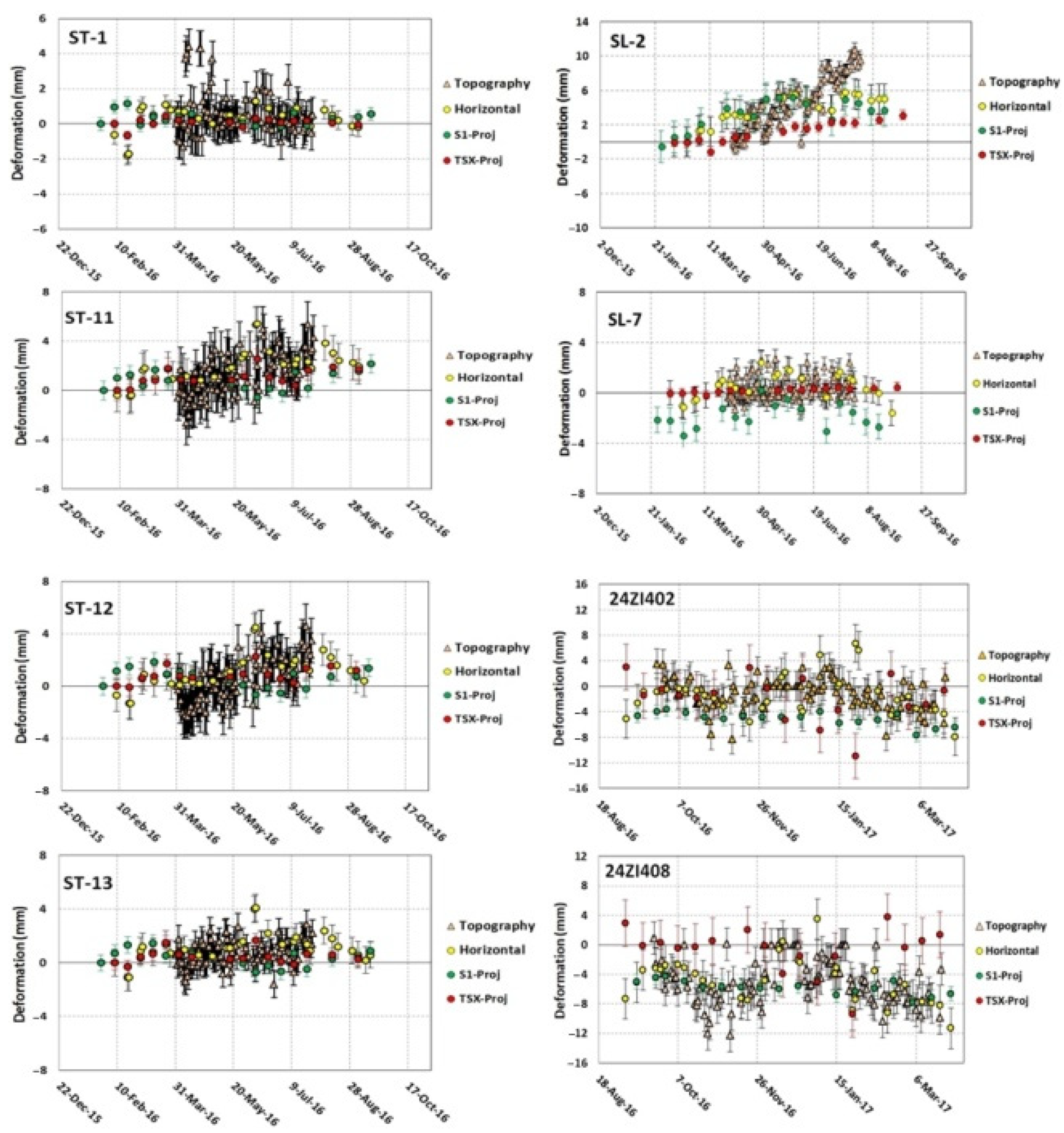
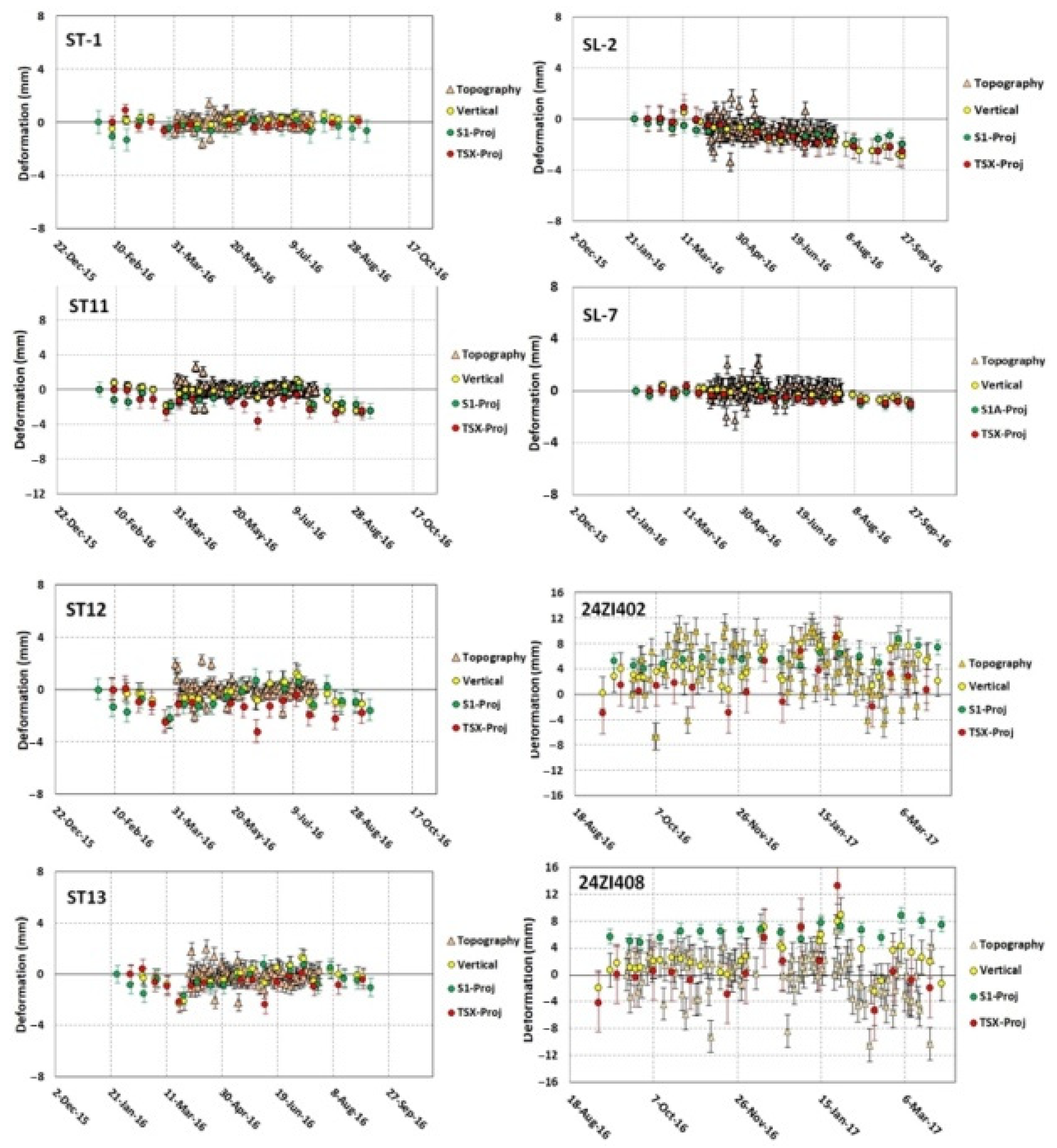
The A-DInSAR analysis was carried out using the SBAS technique [7] using SARSCAPE software version 5.4.1. The differential interferometric phase is the result of the contribution of five phase components related to: topography, displacement, atmosphere, orbit error, and noise [43]. The topographic phase can be partially re-moved using a known digital elevation model (DEM), and the others phase components (atmosphere, orbit error, and noise) can be estimated and removed by proper image stack processing, leaving the phase component referring to the displacement. The phase components of the differential phase can be represented by:
Δ t ( x , r ) = d i s p ( x , r ) + t o p ( x , r ) + a t m ( x , r ) + o r b ( x , r ) + n ( x , r ) ,
where x and r are the azimuth and slant range coordinates, d i s p is the phase shift due to the displacement of the pixel in LoS direction, t o p is the topographic phase error, a t m is the atmospheric phase delay, o r b is the residual phase due to orbit errors and n is due to the phase noise.
In our experiment, the digital elevation model (DEM) used was generated using the rational polynomial coefficients (RPC) model available on the PCI Geomatica OrthoEngine software Version 2018 (PCI Geomatics, Markham, ON, Canada) making full use of the auxiliary parameters of the Pleiades 1-A images acquired on 19 June 2016. This DEM was provided by VISIONA Space Technology Company, with 1 m of spatial resolution, based on triplet of stereoscopic images with spatial resolution of 0.5 m. The methodology used of this procedure is presented in Ostrowski and Cheng [44].
The SBAS approach work with interferograms produced by data pairs characterized by small orbital separation (normal baseline) and small temporal separation (temporal baseline) to limit the spatial and temporal decorrelation effects. The multi-referenced differential interferograms, generated according to the small baseline constraint, are spatially filtered (multi-look) to improve the phase quality to make the process of phase unwrapping easier. The algorithm uses a singular value decomposition (SVD) technique for the inversion to retrieve the average surface deformation velocity and residual topography (First Inversion) and the temporal evolution of surface deformations (Second Inversion) of distributed targets. The availability of a high number of valid interferograms (at least 20) is the basis for the reliability of the estimated products. Figure 2 shows the flow chart of the processing SBAS with TerraSAR-X data and Sentinel-1 data.
The DInSAR data are able to measure variations only in the range direction along the satellite line of sight (LoS). In order to obtain the true displacement component, it is necessary to combine two or more interferometric data stacks acquired over the same area from different geometries. Applying this approach makes it possible to estimate the vertical and horizontal components of the true displacement (def), based on the LoS displacement values (defLoS) and incident angles of both acquisitions for each pixel (Figure 3a) [45,46]. As the satellites move in near polar orbits and the angles of the North–South axis are relatively small, less than 12 degrees, this makes DInSAR too insensitive for measuring components in the North–South direction (Figure 3b), meaning that only deformations in the East–West direction and vertical are feasible.
The TerraSAR (X-band) and Sentinel-1 (C-band) data were used to measure the displacements along the line of sight (LoS) of the Germano mining structures for a period of 16 months in opposite orbits in order for it to be possible to carry out vector decomposition.
A total of 37 single-look complex (SLC) images from Sentinel-1B (S1B) were used, at IW mode, VV polarization, descending orbits, 41.23° incidence angle, 12-day revisit, looking azimuth ~280 degrees (Figure 4b), over a monitoring period from 8 February 2016 to 15 May 2017. Currently, Sentinel-1 imaging is performed systematically in dual mode, with VV and VH polarizations, VV polarization was chosen because VH polarization would have a lower signal level and would be more related to the volume of vegetation.
For the ascending orbits, 37 TerraSAR-X (TSX) images were used for the period of 19 February 2016 to 15 May 2017. These images were acquired in StripMap mode, looking azimuth ~80 degrees (Figure 4b), revisiting time of 11 days, pixel spacing of 1.91 m × 0.91 m (azimuth and range), incidence angle of 35.22°, and covering 30 × 60 km. Figure 4a shows the acquisition schedule of TSX and S1B data, as well as the topographic surveying carried out in two different periods in the test site.
To evaluate the SBAS results, topographic survey (TS) data in situ were used, acquired by a robotic station Leica TM50 (0.6 mm + 1.0 ppm of nominal accuracy) and reflective prisms. Eight prisms installed in different regions, called: ST-1, ST-11, ST-12, ST-13, SL-2, SL-7, 24ZI402 and 24ZI408, installed on the dikes and dam, were chosen to validate the SBAS results. The TS data were carried out and provided by the geotechnical team of SAMARCO Company.
Taking into account that the prisms to total station distances were around 800 m, and the angular errors of the prisms and station were 2.5 s, the nominal TS measurements error was ±8 mm. Since, in theory, the zero reading can present the same nominal error, the established limit of two times the nominal error (accumulated error totalizing 16 mm) was considered as the safety limit for the detection of movements, according to the geotechnical team of the SAMARCO Company.
The TS measurement provided vertical and horizontal values of deformation in different time periods when compared to the TSX and S1B acquisitions. Figure 4a illustrates the different time set of the data, and Figure 4b shows an example of a prism installed in the study area.
For statistical analysis, the Wilcoxon test was performed to verify whether 2D decomposed DInSAR results had similar values to the geotechnical measurements. Wilcoxon is, essentially, a statistical nonparametric test that compares two paired groups and calculates the difference between each set of pairs. This procedure verifies whether two data populations have the same median value and, therefore, can be considered statistically similar. Therefore, if the measurement showed similarity, the SBAS 2D decomposed data may be presumed to be representative of the surface displacement expressed by prism values. This non-parametric statistical test was chosen considering the lack of knowledge of the data distribution and small number of samples.

3. Results

3.1. SBAS Analysis

The TerraSAR-X interferograms were obtained by using a complex multi-look operation with four looks in range and two looks azimuth, normal baseline restriction up to 10% of the critical baseline (6067.34 m) and maximum temporal baseline of 85 days to ensure high interferometric coherence. SBAS processing was performed with a coherence threshold of 0.40, unwrapping using minimum cost flow (MCF) algorithm, and low pass filter (1200 m) for the atmospheric phase removal. The 191 interferograms resulting of the temporal baseline restriction are illustrated in Figure 5a (solid lines). During SBAS processing, 19 interferograms were removed from the 191 generated to achieve better coherence values and lower phase unwrapping errors.
For the SBAS processing of TSX and S1B data, the same distributed ground control points (GCPs) in areas considered stable were used, assuming zero-deformation reference for the refinement/re-flattening of the interferometric phase to perform the second inversion processing. For the refinement and First Inversion processing, 26 distributed GCPs were used, while for the Second Inversion processing, a group of 15 closed GCPs were used, in order to mitigate some linear trends after the first inversion.
For the Sentinel-1 processing data, the maximum normal baseline was 20% of the critical one, and the temporal baseline maximum was 20 days. The multi-looking was performed with eight looks for the range and two for azimuth, the atmospheric low pass filter was 1200 m, and the coherence threshold was 0.26. The 263 interferograms which resulted from the temporal baseline restriction are illustrated in Figure 5b (solid lines). During SBAS processing, 263 interferograms were generated, and 44 of them were removed to have better coherence values and lower phase unwrapping errors. The DEM generated by Pleiades data was used for both TSX and S1 processing. Table 1 shows the acquisition dates of the Reference and Secondary Sentinel-1 data, perpendicular baseline (Bperp) and time interval relative to the Reference image, the Table 2 shows the same information related to the TerraSAR-X data. The processing constraints for both sensors, such as number of looks, atmospheric filter and coherence threshold, were defined after many tests in order to mitigate the phase unwrapping errors.
The displacement rate in the study area can be expressed through the velocity deformation map in LoS (Figure 6) computed with millimetric precision. Positive values correspond to surface motion toward the satellite, negative values correspond to ground motion away from the satellite (red colors), the result is on the Worldview color composite background image. Figure 6 shows the velocity displacement maps of TSX data (Figure 6a) and S1 data (Figure 6b).
The velocity deformation map (mm/y) of TSX data showed a superior number of measured points (MP) (Figure 6a) (2436 MP/km2) compared to the velocity deformation map of Sentinel-1 (Figure 6b) (319 MP/km2). A great part of the study area was stable during the time span of both results showing similar stability behavior of the dikes (greenish colors). A noticeable subsidence was detected by both satellites over the tailings inside of the Baia 3 dike area, with the displacement rate up to −150 mm/year (reddish regions), as well as along the access road on top of Auxiliary Dike 2.
Using the LoS results obtained with the TSX data (ascending orbit) and the S1 satellite (descending orbit), the vector decomposition in the vertical direction as well as in the East–West direction were calculated. The displacement in the vertical direction presented values close to 0 mm on top of the dikes (greenish colors), and close to −80 mm in the tailings inside the Baia 3 dike and the auxiliary dike (reddish regions). The vector decomposition was performed by SARSCAPE software, which considered the MPs closer to the two views to perform the calculations, in this way, the final density of MPs was similar to that of the S1B map. Figure 7 presents the vertical and horizontal displacement maps of the study area obtained by vector decomposition.
The topographic survey (TS) values of vertical and horizontal directions, located on the Selinha dike (SL2, SL7), Sela–Tulipa dikes (ST1, ST11, ST12, ST13), and Germano main dam (24ZI402 and 24ZI408), and the corresponding MPs decomposed, in vertical and horizontal directions (vertical and horizontal) based on the S1 and TSX data, can be seen in the plots of Figure 8 and Figure 9. Additionally, the MPs of S1 and TSX in LoS were projected to the vertical and horizontal directions based on Equations (2) and (3), according to Figure 3a [47], these final values are described as S1-Proj and TSX-Proj in Figure 8 and Figure 9.
v = d e f L o S . cos θ i
h = d e f L o S . sin θ i
where: v = vertical projection, defLoS = deformation value in the line of sight (LoS), θi = incident angle.
The horizontal MP values of the horizontal ground deformation of the prisms locations showed a tendency of deformation of the prisms SL-2, ST-11, ST-12 and ST13 in the East direction (positive values), which the same behavior was noticed of the TS values (Figure 8). The MP values decomposed in the horizontal direction showed a better similarity with the TS horizontal values of the prisms ST-11 and ST-12.
Analyzing the results of the TSX-Proj in the horizontal direction for the prisms SL-2, 24ZI402 and 24ZI408 (Figure 8), it is observed that the MPs’ values did not show good conformity with the TS measurements. In turn, the MPs’ values obtained by the S1-Proj and the horizontal decomposition were closer to the TS data, indicating the dike’s displacement to the East, as observed by in situ survey data.
Figure 9 shows the obtained vertical MPs’ values, corresponding to the crest of the Selinha and Sela–Tulipa dikes, as well as 24ZI402 and 24ZI408 prisms related to the buttress of Germano Dam. In the position of the SL-2 prism (Selinha dike), the TS indicated of subsidence process confirmed by DInSAR results (decomposed and projected).
In turn, all cases on the crest of the Sela–Tulipa dikes, the vertical MPs’ values did not extrapolate the nominal TS measurements error limit (±8 mm) (Figure 9), and thus were considered without the tendency for subsidence or uplift based on this criterion of stability acceptance limit. In SL-7 prism position, the topographic survey (TS) indicated stability in the vertical and horizontal directions, with greater variance in the horizontal direction.
The vertical MPs values obtained by S1-Proj, TSX-Proj and decomposed showed similar results for ST-1, ST11, ST12, ST13, SL-2 and SL7 prisms, with SL-2 presenting a slight tendency to subsidence.
In turn, at 24ZI402 prism position (Germano main dam), the vertical topographic data showed great variability, exceeding the nominal topographic measurements error limit of +/− 8mm. The vertical TSX-Proj MPs showed greater variability and did not agree with the topographic data, while the S1-Proj and vertical decomposition were closer to the topographic data, but not exceeding the error limit.
The vertical TS of 24ZI408 prism (Germano main dam) also showed variability exceeding the nominal topographic measurements error limit of +/− 8mm in four cases. The S1-Proj MPs showed the highest values of surface deformation and uplift. The TSX-Proj MPs showed values close to the topographic data in some cases, but with a great variability. The decomposed vertical values showed a better stability in comparison to the topographic survey during the historical series.
Comparing the mean value of the vertical topographic measurements and the MPs TSX-Proj, S1-Proj and vertical decomposition for each prism, it appears that the mean value of the TSX-Proj (−0.369) was the closest to the TS value (0.408). Analyzing the value of difference between the MPs and the TS reference, it is observed that the vertical decomposed data were the ones that presented the smallest differences between the values (−0.040), and whose mean value was the lowest of the MPs (Table 3).
For the horizontal measurements, it is verified that the mean value of the topographic survey was very low (−0.097), and the horizontal MP TSX-Proj (0.148) was the lower case of radar monitoring. The MPs mean value of the Horizontal Decomposed did not show a value close to the TS (0.610), but this behavior was better than S1-Proj (−0.787). Table 4 shows the comparison of mean values of horizontal deformation obtained by the Horizontal Decomposed and TSX and S1 projected.

3.2. Statistic Test

Wilcoxon test for paired data was carried out for the statistical validation using Statistica v 8.0 software (StatSoft. Inc, Tulsa, OK, USA), in attempt to validate MPS from the decomposition of SBAS measurements with the in situ topographic measurements, represented by eight total stations/prisms measurements (Prism Id). This nonparametric statistical test was chosen due to the small number of samples and the lack of knowledge of the data distribution. Table 5 shows the Wilcoxon results for the decomposed SBAS data (vertical and horizontal decomposition) and the in situ horizontal and vertical deformations, which showed a similarity with the decomposed results and the topographic surveying for all cases analyzed, for 5% significance level.
Analyzing the results of the Wilcoxon statistical test for the vertical projected results obtained TSX-Proj, in 50% of the cases (SL-2, ST1, 24ZI402, 24ZI408) the test indicated similarity with the TS data, considering a significance level of 5% (Table 6). For the results projected in the horizontal direction, the TSX-Proj data presented a better result, with 75% of the cases displaying a similarity with TS (SL-7, ST1, ST11, ST12, ST131 and 24ZI402).
For the vertical results of S1-Proj, in 75% of the cases (SL-2, ST1, ST11, ST12, ST13, and 24ZI402), the Wilcoxon test indicated some similarity with the TS data, considering a significance level of 5%. For the results projected in the horizontal direction, the S1-Proj data showed a similarity with TS in 75% of the cases (SL-2, ST1, ST11, ST12, ST13, and 24ZI408) (Table 7).

4. Discussion

According to statistical validation, the horizontal and vertical measurement points obtained by the vertical and horizontal decomposition provided data compatible with the topographic surveying in situ, and thus can be considered as accurate. Other authors achieved similar success combining different satellite operating data acquired in opposite orbits with the same operating band [47,48,49] and with different bands [46].
In turn, the projected vertical TSX data did not demonstrate a good agreement with the field data of the prisms by the statistical test for most cases, while the projected vertical data S1 obtained a greater degree of acceptance.
For measurements in the horizontal direction, both the projected results of the TSX and S1 showed agreement with the field data, except for two cases, although, all results indicated a similar movement to the East as detected by topographic surveying, mainly for the cases ST-11, SL-2. This deformation in the East direction probably occurred due to the fact that the Germano reservoir was full of tailings, causing pressure on the dikes, while the opposite side was empty after the Fundão dam rupture, thus favoring deformations in this direction. Figure 10a shows the view of the East edge of Tulipa dike, and the Germano reservoir on the opposite side. Figure 10b shows the location and direction from which the photograph was taken, as well as the locations of the prisms ST-11 and ST-12.
It was noticed that the values of the topographic surveying results were very noisy for the prisms 24ZI402 and 24ZI408 (Figure 8 and Figure 9). In both of these prisms, the mean value of the vertical and horizontal decomposed MPs’ measurements followed the TS measurements in great parts of the time series, while the TSX projections did not match with the TS values’ intervals. The S1 projected values overestimated the deformation in the vertical direction (Figure 9).
It is important to emphasize that not all of the MPs’ (projected and decomposed) values obtained exceeded the nominal TS measurements error (±8 mm), reaching the expectations of the geotechnical team of the SAMARCO Company.
The standard deviation values for the vertical decomposition measures showed similar values to the topographic survey. The standard deviation for the TSX-projected measurements was about 64% higher, for the S1-projected vertical measurements the values were lower than the topographic survey.
Analyzing the standard deviation mean values for the decomposed horizontal measurements, the decomposed horizontal, TSX-Proj and S1-proj values were better than those of the topographic survey, due to the multi-looking processing. It is important to point out that the period of November 2016 to February 2017 was in the rainy season in the study region, which reached an accumulated rainfall of 280 mm, which increased the standard deviation values of the topographic survey and the DInSAR results.
In order to analyze the temporal changes and the pluviometry influence, the multitemporal coherence was carried out [50,51], and the prism locations’ values were compared to the local pluviometry. For the Sentinel case, it was noticed that the rainy season affected the coherence behavior (Figure 11), decreasing its values, while in the drought season the coherence values were more stable with higher values.
For the TerraSAR-X case, the behavior of the coherence against the rainfall data was similar, but with a stronger effect for the coherence values during the longer periods of higher rainfall values (Figure 12), causing a significant decrease in coherence. During the dry season, the coherence showed higher values. The difference in resolution and the wavelength between the sensors is likely to be the reason for the more sensitive TerraSAR-X data with the pluviometry.
The vertical deformations detected on the auxiliary dikes may be due to the geomechanical differences between the dikes and dams, associated with the machine traffic on their structure and their continuous maintenance.
Surface vertical displacements were detected on the reservoir of Baia 3, which reached accumulated values up to -80 mm due to the tailings settlement (Figure 7a), since there was no deposition of waste material in the reservoir after the Fundão dam rupture, no horizontal movements were observed inside the Baia 3 reservoir (Figure 7b).

5. Conclusions

The results obtained with the vector decomposition in the vertical and horizontal directions (East–West) based on the LoS measurements from different sensors were similar to the topographic data collected in the field. Due to the satellite acquisition geometry, horizontal deformations in the North–South direction cannot be measured with sufficient accuracy because it not perceptible.
The density of MPs using Sentinel-1 data was lower than using TerraSAR-X data, but it was still possible to obtain coherent measurements in the dikes and dam, which allowed us to perform vector decomposition and estimate the vertical and horizontal deformations.
It should be noted that the Sentinel-1 satellite coverage of the Brazilian territory usually occurs in the ascending or descending orbit, and thus does not have the possibility of a historical series of opposite sight to develop the technique of this article, meaning that the combination of the use of data from another sensor allows its execution. In turn, the measurements projected provide interesting measurements, which, according to the criteria of Samarco’s geotechnical team, met the acceptance interval; despite the theory that the measurements projected are more accurate when the ground deformations occur only in the vertical direction.
Finally, due to the large number of tailings dams in different regions of Brazil, unmonitored or with deficient monitoring systems, there is a significant demand for information on deformations mainly related to the tailings dams due to legal obligations, safety, and environmental monitoring, etc. The use of the A-DInSAR technique using opposite tracks data proved to be an effective tool for providing key information to help make crucial decisions regarding risks, or even mitigation, repairs or emergency response in circumstances that can lead to loss of life and damages to infrastructure and the environment.

Author Contributions

F.F.G. and A.C. were in charge of SAR processing; F.F.G., A.C. and J.C.M. carried out the analysis of results and wrote the manuscript. All authors have read and agreed to the published version of the manuscript.

Funding

This research was funded by Agência Espacial Brasileira (AEB) and Instituto Nacional de Pesquisas Espaciais (INPE).

Data Availability Statement

The Sentinel-1 data was available by the ESA Hub, and the TerraSAR-X data was provided the VISIONA TECNOLOGIA ESPACIAL S.A. and AIRBUS DEFENCE & SPACE companies.

Acknowledgments

The authors are grateful for the support of VISIONA TECNOLOGIA ESPACIAL S.A. and AIRBUS DEFENCE & SPACE companies by providing the TerraSAR-X and Pleiades images for this research, and the SAMARCO Mineração S.A. for providing the topographic data and supporting the field campaign.

Conflicts of Interest

The authors declare no conflict of interest.

Abbreviations

ANMAgencia Nacional de Mineração (Brazilian National Mining Agency)
A-DInSARAdvanced- Differential Interferometric Synthetic Aperture Radar
BperpPerpendicular baseline
DEMDigital elevation model
ENVIEnvironment for Visualizing Images
GCPGround Control Points
LoSLine of sight
MPMeasured points
QFQuadrilátero Ferrífero (Iron Quadrangle)
SARSynthetic Aperture Radar
SBASSmall BAseline Subset
SVDSingular value decomposition
TSTopographic Survey

References

  1. ANM. Tailings Dam Classification and Safety Plan. 2019. Available online: http://www.anm.gov.br/assuntos/barragens/pasta-classificacao-de-barragens-demineracao/plano-de-seguranca-de-barragens (accessed on 9 June 2019).
  2. Kossoff, D.; Dubbin, W.E.; Alfredsson, M.; Edwards, S.J.; Macklin, M.G.; Hudson-Edwards, K.A. Mine Tailings Dams: Characteristics, Failure, Environmental Impacts, and Remediation. Appl. Geochem. 2014, 51, 229–245. [Google Scholar] [CrossRef] [Green Version]
  3. Morgenstern, N.R.; Vick, S.G.; Viotti, C.B.; Watts, B.D. Fundão Tailings Dam Review Panel: Report on the Immediate Causes of the Failure of the Fundão Dam. pp76. 2016. Available online: https://pedlowski.files.wordpress.com/2016/08/fundao-finalreport.pdf (accessed on 2 August 2022).
  4. Jaroz, A.; Wanke, D. Use of InSAR for Monitoring of Mining Deformations. In Proceedings of the Fringe Workshop 2003, Frascati, Italy, 1–5 December 2003. [Google Scholar]
  5. Crosetto, M.; Crispa, B.; Biescas, E.; Monserrat, O.; Agudo, M.; Fernandes, P. Land Deformation Monitoring Using SAR Interferometry: State-of-the-art. Photogramm. Fernerkund. Geoinf. 2005, 6, 497–510. [Google Scholar]
  6. Ferretti, A.; Prati, C.; Rocca, F. Permanent scatterers in SAR interferometry. IEEE Trans. Geosci. Remote Sens. 2001, 39, 8–20. [Google Scholar] [CrossRef]
  7. Berardino, P.; Fornaro, G.; Lanari, R.; Sansosti, E. A new algorithm for surface deformation monitoring based on small baseline differential SAR interferograms. IEEE Trans. Geosci. Remote Sens. 2002, 40, 2375–2383. [Google Scholar] [CrossRef] [Green Version]
  8. Paradella, W.R.; Ferretti, A.; Mura, J.C.; Colombo, D.; Gama, F.F.; Tamburini, A.; Santos, R.A.; Novalli, F.; Galo, M.; Camargo, P.O.; et al. Mapping surface deformation in open pit iron mines of Carajás Province (Amazon Region) using an integrated SAR analysis. Eng. Geol. 2015, 193, 61–78. [Google Scholar] [CrossRef] [Green Version]
  9. Herrera, G.; Tomás, R.; Vicente, F.; Lopez-Sanchez, J.M.; Mallorquí, J.J.; Mulas, J. Mapping ground movements in open pit mining areas using differential SAR interferometry. Int. J. Rock Mech. Min. Sci. 2010, 47, 1114–1125. [Google Scholar] [CrossRef]
  10. Przyłucka, M.; Herrera, G.; Graniczny, M.; Colombo, D.; Béjar-Pizarro, M. Combination of Conventional and Advanced A-DInSAR to Monitor Very Fast Mining Subsidence with TerraSAR-X Data: Bytom City (Poland). Remote Sens. 2015, 7, 5300–5328. [Google Scholar] [CrossRef] [Green Version]
  11. Tang, W.; Motagh, M.; Zhand, W. Monitoring active open-pit mine stability in the Rhenish coalfields of Germany using a coherence-based SBAS method. Int. J. Appl. Earth Obs. Geoinf. 2020, 93, 102217. [Google Scholar] [CrossRef]
  12. Hartwig, M.E.; Paradella, W.R.; Mura, J.C. Detection and monitoring of surface motions in active mine in the Amazon region, using persistent scatterer interferometry with TerraSAR-X satellite Data. Remote Sens. 2013, 5, 4719–4734. [Google Scholar] [CrossRef] [Green Version]
  13. Pinto, C.A.; Paradella, W.R.; Mura, J.C.; Gama, F.F.; Santos, A.R.; Silva, G.G.; Hartwig, M.E. Applying persistent scatterer interferometry for surface displacement mapping in the Azul open pit manganese mine (Amazon region) with TerraSAR-X data. J. Appl. Remote Sens. 2015, 9, 095978-18. [Google Scholar] [CrossRef] [Green Version]
  14. Mura, J.C.; Paradella, W.R.; Gama, F.F.; Silva, G.G.; Galo, M.; Camargo, P.; Silva, A. Monitoring of Non Linear Ground Movement in an Open Pit Iron Mine Based on an Integration of Advanced DInSAR Techniques Using TerraSAR-X Data. Remote Sens. 2016, 8, 409. [Google Scholar] [CrossRef]
  15. Silva, G.G.; Mura, J.C.; Paradella, W.R.; Gama, F.F.; Temporin, F.A. Monitoring of ground movement in open pit iron mines of Carajás Province (Amazon region) based on A-DInSAR techniques using TerraSAR-X data. J. Appl. Remote Sens. 2017, 11, 026027. [Google Scholar] [CrossRef] [Green Version]
  16. Gama, F.F.; Cantone, A.; Mura, J.C.; Pasquali, P.; Paradella, W.R.; Santos, A.R.; Silva, G.G. Monitoring subsidence of open pit iron mines at Carajás Province based on SBAS interferometric technique using TerraSAR-X data. Remote Sens. Appl. Soc. Environ. 2017, 8, 199–211. [Google Scholar] [CrossRef]
  17. Mura, J.C.; Gama, F.F.; Paradella, W.R.; Negrão, P.; Carneiro, S.; Oliveira, C.G.; Brandão, W.S. Monitoring the vulnerability of the dam and dikes in Germano iron mining after the collapse of the tailings dam of Fundão (Mariana-MG, Brazil) using DInSAR techniques with TerraSAR-X data. Remote Sens. 2018, 10, 1507. [Google Scholar] [CrossRef] [Green Version]
  18. Gama, F.F.; Paradella, W.R.; Mura, J.C.; Oliveira, C.G. Advanced DInSAR analysis on dam stability monitoring: A case study in the Germano mining complex (Mariana, Brazil) with SBAS and PSI techniques. Remote Sens. Appl. Soc. Environ. 2019, 16, 100267. [Google Scholar] [CrossRef]
  19. Gama, F.F.; Mura, J.C.; Paradella, W.R.; Oliveira, C.G. Deformations Prior to the Brumadinho Dam Collapse Revealed by Sentinel-1 InSAR Data Using SBAS and PSI Techniques. Remote Sens. 2020, 12, 3664. [Google Scholar] [CrossRef]
  20. Mura, J.C.; Gama, F.F.; Paradella, W.R.; Oliveira, C.G.; Rodrigues, T.G. Ground displacements revealed by A-DInSAR analysis in the Germano iron mining complex before and after the Fundão Dam collapse using Sentinel-1 data. J. Appl. Remote Sens. 2021, 15, 036513-19. [Google Scholar] [CrossRef]
  21. Krishnakumar, V.; Qiu, Z.; Monserrat, O.; Barra, A.; López-Vinielles, J.; Reyes-Carmona, C.; Gao, Q.; Cuevas-González, M.; Palamà, R.; Crippa, B.; et al. Sentinel-1 A-DInSAR Approaches to Map and Monitor Ground Displacements. Remote Sens. 2021, 13, 1120. [Google Scholar] [CrossRef]
  22. Du, Z.; Ge, L.; Ng, A.H.M.; Li, X. Investigation on mining subsidence over Appin–West Cliff Colliery using time-series SAR interferometry. Int. J. Remote Sens. 2017, 39, 1528–1547. [Google Scholar] [CrossRef]
  23. Pawluszek-Filipiak, K.; Borkowski, A. Monitoring mining induced subsidence by integrating differential radar interferometry and persistent scatterer techniques. Eur. J. Remote Sens. 2021, 54, 18–30. [Google Scholar] [CrossRef]
  24. Colesanti, C.; Mouelic, S.L.; Bennani, M.; Raucoules, D.; Carnec, C.; Ferretti, A. Detection of mining related ground instabilities using the Permanent Scatterers technique: A case study in the east of France. Int. J. Remote Sens. 2005, 26, 201–207. [Google Scholar] [CrossRef]
  25. Perski, Z.; Hanssen, R.; Wojcik, A.; Wojciechowski, T. InSAR analyses of terrain deformation near the Wieliczka Salt Mine, Poland. Eng. Geol. 2009, 106, 58–67. [Google Scholar] [CrossRef]
  26. Guéguen, Y.; Deffontaines, B.; Fruneau, B.; Al Heib, M.; Michele, M.; Raucoules, D.; Guise, Y.; Planchenault, J. Monitoring residual mining subsidence of Nord/Pas-de-Calais coal basin from differential and Persistent Scatterer Interferometry (Northern France). J. Appl. Geophys. 2009, 69, 24–34. [Google Scholar] [CrossRef]
  27. Ng, A.-H.M.; Ge, L.; Yan, Y.; Li, X.; Chang, H.-C.; Zhang, K.; Rizos, C. Mapping accumulated mine subsidence using small stack of SAR differential interferograms in the Southern coalfield of New South Wales, Australia. Eng. Geol. 2010, 115, 1–15. [Google Scholar] [CrossRef]
  28. Zhang, Z.; Tang, Y.; Zhang, H.; Wang, C.; Fu, Q. Subsidence monitoring in coal area using time-series InSAR combining persistent scatterers and distributed scatterers. Int. J. Appl. Earth Obs. Geoinf. 2015, 39, 49–55. [Google Scholar] [CrossRef]
  29. Wegmüller, U.; Walter, D.; Spreckels, V.; Werner, C.L. Nonuniform ground motion monitoring with TerraSAR-X persitent scatterer interferometry. IEEE Trans. Geosci. Remote Sens. 2010, 48, 895–904. [Google Scholar] [CrossRef]
  30. Raucoles, D.; Maisons, C.; Carnec, C.; Le Mouelic, S.; King, C.; Hosford, S. Monitoring of slow ground deformation by ERS radar interferometry on Vauvert salt mine (France). Remote Sens. Environ. 2003, 88, 468–478. [Google Scholar] [CrossRef]
  31. Jung, H.C.; Kim, S.-W.; Jung, H.-S.; Min, K.D.; Won, J.-S. Satellite observation of coal mining subsidence by persistent scatterer analysis. Eng. Geol. 2007, 92, 1–13. [Google Scholar] [CrossRef]
  32. Agurto-Detzel, H.; Bianchi, M.; Assumpção, M.; Schimmel, M.; Collaço, B.; Ciardelli, C.; Barbosa, J.R.; Calhau, J. The tailings dam failure of 5 November 2015 in SE Brazil and its preceding seismic sequence. Geophys. Res. Lett. 2016, 43, 4929–4936. [Google Scholar] [CrossRef] [Green Version]
  33. Escobar, H. Mud tsunami wreaks ecological havoc in Brazil. Science 2015, 350, 1138–1139. [Google Scholar] [CrossRef]
  34. Garcia, L.C.; Ribeiro, D.B.; Roque, F.O.; Ochoa-Quintero, J.M.; Laurance, W.F. Brazil’s worst mining disaster: Corporations must be compelled to pay the actual environmental costs. Ecol Appl. 2016, 27, 5–9. [Google Scholar] [CrossRef] [PubMed]
  35. Devanthéry, N.; Crosetto, M.; Monserrat, O.; Cuervas-Gonzales, M.; Crippa, B. Deformation Monitoring using Sentinel-1 SAR Data. In Proceedings of the 2nd International Electronic Conference on Remote Sensing (SCIforum), Basel, Switzerland, 22 March–5 April 2018; Volume 2. [Google Scholar]
  36. Strozzi, T.; Antonova, S.; Günther, F.; Mätzler, E.; Gonçalo Vieira, G.; Wegmüller, U.; Westermann, S.; Bartsch, A. Sentinel-1 SAR Interferometry for Surface Deformation Monitoring in Low-Land Permafrost Areas. Remote Sens. 2018, 10, 1360. [Google Scholar] [CrossRef] [Green Version]
  37. Intrieri, E.; Raspini, F.; Fumagalli, A.F.; Lu, P.; Conte, D.C.; Farina, P.; Allievi, J.; Ferretti, A.; Casagli, N. The Maoxian landslide as seen from space: Detecting precursors of failure with Sentinel-1 data. Landslides 2018, 15, 123–133. [Google Scholar] [CrossRef] [Green Version]
  38. Béjar-Pizarro, M.; Notti, D.; Mateos, R.M.; Ezquerro, P.; Centolanza, G.; Herrera, G.; Bru, G.; Sanabria, M.; Solari, L.; Javier Duro, J.; et al. Mapping Vulnerable Urban Areas Affected by Slow-Moving Landslides Using Sentinel-1 InSAR Data. Remote Sens. 2017, 9, 876. [Google Scholar] [CrossRef] [Green Version]
  39. Lanari, R.; Bonano, M.; Buonanno, S.; Casu, F.; De Luca, C.; Fusco, A.; Manunta, M.; Manzo, M.; Onorato, G.; Zeni, G.; et al. Continental Scale SBAS-DInSAR Processing for the Generation of Sentinel-1 Deformation Time Series within a Cloud Computing Environment: Achieved Results and Lessons Learned. In Proceedings of the EGU General Assembly 2020, Online, 4–8 May 2020. [Google Scholar] [CrossRef]
  40. Almeida, F.F.M.A. O Craton do São Francisco. Rev. Bras. Geoc. 1977, 7, 349–364. [Google Scholar]
  41. Dorr, J.V.N., II. Physiographic, Stratigraphic and Structural Development of the Quadrilátero Ferrífero; Geological Survey Professional Paper; United States Government Publishing Office: Washington, DC, USA, 1969.
  42. Castilho, B.M. Análise dos Gatilhos de Liquefação Dinâmica e Modelagem Numérica da Barragem do Germano. Master’s Thesis, Geotechnical Engineering, Federal University of Ouro Preto, Ouro Preto, Brazil, 2017. [Google Scholar]
  43. SARscape Technical Description. 2012. Available online: http://www.sarmap.ch/pdf/SARscapeTechnical.pdf (accessed on 5 July 2020).
  44. Ostrowski, J.A.; Cheng, P. DEM Extraction from Stereo SAR Satellite Imagery. In Proceedings of the IGARSS’2000: Proceedings of the International Geoscience and Remote Sensing Symposium, Honolulu, Hawaii, 25–28 July 2000; IEEE: New York, NY, USA, 2000. [Google Scholar]
  45. Ferretti, A. Satellite InSAR Data: Reservoir from Space; EAGE Publications: Bunnik, The Netherlands, 2014. [Google Scholar]
  46. Yu, L.; Yang, T.; Zhao, Q.; Liu, M.; Pepe, A. The 2015–2016 Ground Displacements of the Shanghai Coastal Area Inferred from a Combined COSMO-SkyMed/Sentinel-1 DInSAR Analysis. Remote Sens. 2017, 9, 1194. [Google Scholar] [CrossRef] [Green Version]
  47. Bayramov, E.; Buchroithner, M.; Kada, M.; Zhuniskenov, Y. Quantitative Assessment of Vertical and Horizontal Deformations Derived by 3D and 2D Decompositions of InSAR Line-of-Sight Measurements to Supplement Industry Surveillance Programs in the Tengiz Oilfield (Kazakhstan). Remote Sens. 2021, 13, 2579. [Google Scholar] [CrossRef]
  48. Dai, K.; Liu, G.; Li, Z.; Li, T.; Yu, B.; Wang, X.; Singleton, A. Extracting Vertical Displacement Rates in Shanghai (China) with Multi-Platform SAR Images. Remote Sens. 2015, 7, 9542–9562. [Google Scholar] [CrossRef] [Green Version]
  49. Ng, A.; Ge, L.; Zhang, K.; Li, X. Estimating horizontal and vertical movements due to underground mining using ALOS PALSAR. Eng. Geol. 2012, 143, 18–27. [Google Scholar] [CrossRef]
  50. Manzoni, M.; Molinari, M.E.; Monti-Guarnieri, A. Multitemporal InSAR Coherence Analysis and Methods for Sand Mitigation. Remote Sens. 2021, 13, 1362. [Google Scholar] [CrossRef]
  51. Boccardo, P.; Gentile, V.; Giulio-Tonolo, F.; Grandoni, D.; Vassileva, M. Multitemporal SAR Coherence Analysis: Lava Flow Monitoring Case Study. In Proceedings of the 2015 IEEE International Geoscience and Remote Sensing Symposium (IGARSS), Milan, Italy, 26–31 July 2015. [Google Scholar] [CrossRef]
Figure 1. Germano iron complex location in Mariana/MG; the background image was obtained from Google Earth.
Mining 02 00040 g001
Figure 2. Data processing flow chart.
Mining 02 00040 g002
Figure 3. (a) Vertical and horizontal displacement obtained by 2D decomposition of the ascending and descending data (East-West direction), (b) imaging trajectory geometries (North-South direction).
Mining 02 00040 g003
Figure 4. (a) Plot of acquisition of TSX and S1B images and topographic surveying with prisms; (b) Example of prism used on the topographic surveying.
Mining 02 00040 g004
Figure 5. Interferometric pairs selected (solid blue lines): (a) TSX pairs, (b) S1B pairs. Yellow dot means reference image.
Mining 02 00040 g005
Figure 6. Velocity displacement map in LoS: (a) TSX data, (b) S1B data. The orange triangles represent the position of the prims used for the topographic surveying.
Mining 02 00040 g006
Figure 7. Maps of displacement: (a) Vertical, (b) Horizontal.
Mining 02 00040 g007
Figure 8. Horizontal ground deformation of the prisms locations (MP projected and MP decomposed) and TS (horizontal topographic measurements): ST-1; ST-11; ST-12; ST-13, SL-2; SL-7; 24ZI402; 24ZI408.
Mining 02 00040 g008
Figure 9. Vertical ground deformation of the prisms locations (MP projected and MP decomposed) and TS (vertical topographic measurements): ST-1; ST-11; ST-12; ST-13, SL-2; SL-7; 24ZI402; 24ZI408.
Mining 02 00040 g009
Figure 10. (a) View from the East edge of the Tulipa dike, with the Germano Reservoir on the opposite side (West), (b) position and direction from which the photo was taken, as well as the locations of the prisms ST-11 and ST-12.
Mining 02 00040 g010
Figure 11. Multitemporal S1 coherence and local pluviometry.
Mining 02 00040 g011
Figure 12. Multitemporal TSX coherence and local pluviometry.
Mining 02 00040 g012
Table 1. The acquisition dates of the Reference and Secondary S1B images, perpendicular baseline (Bperp) and time interval relative to the Reference image.
PairReference *Secondary *Bperp (m)PairReference *Secondary *Bperp (m)
120,160,72520,160,20877.191920,160,72520,161,01186.51
220,160,72520,160,220109.292020,160,72520,161,023156.47
320,160,72520,160,303150.442120,160,72520,161,104126.05
420,160,72520,160,327152.912220,160,72520,161,116146.96
520,160,72520,160,408155.022320,160,72520,161,12858.46
620,160,72520,160,42088.952420,160,72520,161,21053.81
720,160,72520,160,502122.832520,160,72520,161,222110.06
820,160,72520,160,514156.842620,160,72520,170,103143.79
920,160,72520,160,52685.112720,160,72520,170,115135.87
1020,160,72520,160,60793.292820,160,72520,170,127132.80
1120,160,72520,160,701153.122920,160,72520,170,20891.44
1220,160,72520,160,71386.203020,160,72520,170,22054.12
1320,160,72520,160,806112.953120,160,72520,170,304127.22
1420,160,72520,160,818132.123220,160,72520,170,31657.73
1520,160,72520,160,83097.263320,160,72520,170,328136.14
1620,160,72520,160,91136.883420,160,72520,170,40995.16
1720,160,72520,160,923141.713520,160,72520,170,503143.40
1820,160,72520,160,929171.883620,160,72520,170,515177.83
Obs: * yyyymmdd, Critical baseline = 5951.63 m.
Table 2. The acquisition dates of the Reference and Secondary TSX images, perpendicular baseline (Bperp) and time interval relative to the Reference image.
PairReference *SecondaryBperp (m)PairReference *SecondaryBperp (m)
120,161,22320,160,208206.971920,161,22320,161,01825.95
220,161,22320,160,219−90.4532020,161,22320,161,029−136.30
320,161,22320,160,301−270.612120,161,22320,161,120−36.22
420,161,22320,160,312−80.172220,161,22320,161,201−59.65
520,161,22320,160,323−352.082320,161,22320,161,21236.05
620,161,22320,160,403−206.972420,161,22320,161,223−218.95
720,161,22320,160,414−225.402520,161,22320,170,103−108.69
820,161,22320,160,517−331.952620,161,22320,170,11429.08
920,161,22320,160,528−349.372720,161,22320,170,125−297.55
1020,161,22320,160,608−54.8132820,161,22320,170,216340.65
1120,161,22320,160,619−261.252920,161,22320,170,227134.90
1220,161,22320,160,630−329.683020,161,22320,170,310207.28
1320,161,22320,160,711−158.703120,161,22320,170,321250.29
1420,161,22320,160,722−175.933220,161,22320,170,401178.15
1520,161,22320,160,813−57.703320,161,22320,170,41280.78
1620,161,22320,160,904−87.703420,161,22320,170,42316.22
1720,161,22320,160,915−41.053520,161,22320,170,504−25.74
1820,161,22320,160,926−55.453620,161,22320,170,515115.67
Obs: * yyyymmdd, Critical baseline = 6067.76 m.
Table 3. Comparison of values of vertical displacement.
SL-2SL-7ST1ST11ST12ST1324ZI40224ZI408MeanSD
TS (vertical) *−0.6500.3770.0310.103−0.197−0.0834.221−0.5360.4080.959
Vertical decomp *−1.36−0.1790.1240.028−0.197−0.0114.717−0.1760.3681.005
Vertical decomp- TS *−0.712−0.5560.093−0.0750.0000.0720.4960.360−0.0400.047
TSX- Proj *−1.309−0.561−0.257−1.608−1.347−0.7131.8321.014−0.3691.498
TSX- Proj-TS *−0.659−0.938−0.288−1.711−1.150−0.630−2.3891.550−0.7770.539
S1- Proj *−1.075−0.522−0.217−0.415−0.415−0.1895.7555.7211.0800.746
S1- Proj-TS *−0.425−0.899−0.248−0.518−0.218−0.1061.5346.2570.672−0.213
* milimeters (mm); TS: Topographic Survey; SD: Standart Deviation Mean value.
Table 4. Comparison of values of horizontal displacement.
SL-2SL-7ST1ST11ST12ST1324ZI40224ZI408MeanSD
TS (horizontal) *4.0440.407−0.1091.8970.6130.153−1.704−6.079−0.0971.833
Horizontal decomp *4.5340.9990.4742.2971.5581.531−1.380−5.1350.6101.455
Horizontal decomp- TS *−0.490−0.592−0.583−0.400−0.945−1.378−0.324−0.944−0.707−0.377
TSX- Proj *0.9260.2990.1531.1360.9510.504−2.066−0.7190.1481.222
TSX- Proj-TS *3.1180.108−0.2620.761−0.338−0.3510.362−5.360−0.245−0.611
S1- Proj *4.292−1.8611.1910.4300.3650.053−5.044−5.721−0.7870.908
S1- Proj-TS *−0.2482.268−1.3001.4670.2480.1003.340−0.3580.690−0.924
* milimeters (mm); TS: Topographic Survey; SD: Standart Deviation Mean value.
Table 5. Wilcoxon statistic test of the vertical and horizontal decomposed data.
Vertical DecompositionHorizontal Decomposition
Prism IdN
(Cases)
T
(W Test)
p-Valueμ1 = μ2T
(W Test)
p-Valueμ1 = μ2
SL-218440.071 Ok 850.982Ok
SL-718410.053 Ok 420.058Ok
ST11875.50.663 Ok 440.071Ok
ST1118810.844 Ok 430.064Ok
ST1218770.711 Ok 410.053Ok
ST1318740.615 Ok 470.093Ok
24ZI402271650.564 Ok 1760.755Ok
24ZI408271690.630 Ok 1140.072Ok
Significance level: p < 0.05; number of cases: N; Wilcoxon test: T; median of a group of data: μ.
Table 6. Wilcoxon statistic test of the vertical and horizontal TSX-Proj.
Vertical DirectionHorizontal Direction
Prism IdN
(Cases)
T
(W Test)
p-Valueμ1 = μ2T
(W Test)
p-Valueμ1 = μ2
SL-29120.213Ok10.011.Not Ok
SL-7950.038Not Ok210.859Ok
ST1970.066Ok120.213Ok
ST11910.011Not Ok100.138Ok
ST12920.015Not Ok190.678Ok
ST13950.038Not Ok150.374Ok
24ZI40214340.245Ok470.729Ok
24ZI40814360.300Ok100.008Not Ok
Significance level: p < 0.05; number of cases: N; Wilcoxon test: T; median of a group of data: μ.
Table 7. Wilcoxon statistic test of the vertical and horizontal S1-Proj.
Vertical DirectionHorizontal Direction
Prism IdN
(Cases)
T
(W Test)
p-Valueμ1 = μ2T
(W Test)
p-Valueμ1 = μ2
SL-2990.109Ok210.858Ok
SL-7920.015Not Ok20.015Not Ok
ST19100.139Ok130.260Ok
ST11990.139Ok80.085Ok
ST129140.314Ok180.594Ok
ST139190.678Ok210.859Ok
24ZI40214230.064Ok10.001Not Ok
24ZI4081410.001Not Ok380.363Ok
Significance level: p < 0.05; number of cases: N; Wilcoxon test: T; median of a group of data: μ.
Publisher’s Note: MDPI stays neutral with regard to jurisdictional claims in published maps and institutional affiliations.

