Proceeding Paper

GIS-Based Groundwater Potentiality Mapping Using AHP and FR Models in Central Antalya, Turkey †

1
Department of Remote Sensing and Geographic Information System, Graduate School of Sciences, Eskisehir Technical University, Eskisehir 26000, Turkey
2
Department of Geological Engineering and Exploration of Mines, Faculty of Geology and Mining, Kabul Polytechnic University, Kabul 1001, Afghanistan
3
Institute of Earth & Space Sciences, Eskisehir Technical University, Eskisehir 26000, Turkey
*
Author to whom correspondence should be addressed.
Presented at the 3rd International Electronic Conference on Geosciences, 7–13 December 2020; Available online: https://iecg2020.sciforum.net/.
Environ. Sci. Proc. 2021, 5(1), 11; https://doi.org/10.3390/IECG2020-08741
Published: 1 December 2020

Abstract

:
Groundwater is considered one of the essential natural resources stored beneath the earth’s surface by infiltration through various rock layers. Groundwater potential supplies almost 30% of fresh water globally, and in general, 65% of groundwater is used for agricultural irrigation, 25% as drinking water, and the remaining 10% is utilized as industrial water. This study aimed to delineate potential groundwater zones in the central Antalya province, Turkey, using the analytical hierarchy process (AHP) and frequency ratio (FR). Seven thematic layers, including lithology, slope, drainage density, landcover/land use, lineament density, rainfall, and soil depth, were considered as influencing factors for these models. The preparation of all geospatial datasets was carried out in the GIS environment and Google Earth Engine. Additionally, some authorized relevant web portals were also tried for obtaining the required spatial data. The findings of analysis by AHP and FR models showed that Muratpasa, Kepez, and eastern Dosemealti in the eastern part of the study area are characterized by a high potentiality of groundwater. In contrast, the regions in the southern and the western parts covered by igneous rocks and other less permeable sediments, also featuring high and steep slopes, were also followed by a low or very low groundwater potential. Consequently, the results from both models were assessed using the receiver operating curve (ROC) and area under the curve (AUC) for validation. The validation in this study confirmed the higher effectivity of the results achieved by FR than the AHP model.

1. Introduction

Groundwater is considered one of the vital elements of nature found in the voids of the earth and packs the pore space of soil beneath the water table [1,2,3,4]. Groundwater is proven to be one of the most significant natural resources, which is an essential source of water supply in all climatic regions of the world [5,6]. Almost 30% of the world’s fresh water is supplied by groundwater, while only 0.3% is furnished by surface water, including lakes, reservoirs, and rivers [4,7]. The primary groundwater sources are rainwater and snowmelt, which leach down through the soil pores into the aquifer [8].
At present, due to the rapid growth of industrialization and the population, there is an increasing demand for fresh water, which directly affects groundwater availability. This is a worldwide concern. Therefore, groundwater exploitation is considered an essential part of water management and planning [4,7]. The availability of groundwater resources depends on the diverse geological, morphological, biological, and atmospheric characteristic factors, including lithology, topographic conditions, geological structures, climate, soil type, and many others; however, the movement mainly depends on the porosity, permeability, transmissibility, and storage capacity of the rocks [9,10,11,12].
There are several approaches for targeting groundwater potential by considering these factors. The applicable methods are geological, geophysical, and remote sensing, which many scientists examined. The efficiency of the methods is varied; some of them are more effective, accurate, time-saving, and less expensive, while the traditional methods are time-consuming and require high expenses [13,14,15]. Furthermore, the integration of GIS and remote sensing studies makes it possible to analyze and store large amounts of geospatial data and delineate groundwater potential using different methods [4,15,16].
Several studies were carried out for groundwater management, using various multicriteria decision-making and machine learning algorithms [12,13,17,18,19]. Diverse studies were undertaken on groundwater potential mapping, using the analytical hierarchy process (AHP), frequency ratio (FR), and influencing factor [4,15,20,21,22,23,24,25,26]. Some other researchers examined the logistic model tree, the Dempster–Shafer model, the certainty factor, logistic regression, the random forest model, the maximum entropy model, the decision tree model, and artificial neural networks to delineate groundwater potentiality [27,28,29,30,31].
Central Antalya is covered mainly by agricultural areas consuming groundwater reservoirs; furthermore, in some areas, groundwater is characterized by pollutants. Due to the Mediterranean climate, the study area is characterized by hot and dry weather in summer and warm weather in winter. Hence, distinct groundwater management and planning are required to overcome the problems arising from drought. The initial planning highlights the groundwater potentiality mapping. Therefore, this study aims to delineate the groundwater potential zones using the AHP and FR models in a GIS environment. The findings of this study sufficiently contribute to further detailed groundwater-related studies, agricultural irrigation planning, and urban planning in the Antalya province.

2. Study Area

Central Antalya is located in the southwestern part of Turkey, within the longitudes 29°44/–35°52/ and the latitudes 36°41/–37°20/, over the Antalya Travertine Plateau. It contains an area of almost 4060 km2, which covers the 5 districts Korkuteli, Dosemealti, Kepez, Muratpasa, and Konyaalti. Regionally, the study area borders the Sparta, Burdur, and Denizli provinces, the Toros Mountains in the north, and the Mediterranean Sea in the southeast (Figure 1). The study area was characterized by the Mediterranean climate—hot and dry in summer and warm and rainy in winter.

3. Material and Methods

A geographic information system and remote sensing were used in this study to map groundwater potential zones by examining analytical hierarchy process and frequency ratio models. In total, seven thematic layers including lithology, slope, drainage density, landcover/land use, lineament density, rainfall, and soil depth were generated and weighted considering the expert ideas and previous literature. The whole design of the methodology is depicted in Figure 2.

3.1. Generation of Geospatial Datasets

Remotely sensed, conventional, and climatic data were provided from different organizations and authorized websites to generate thematic layers influencing the groundwater potential. The lithology of an area is the most critical factor while considering groundwater potential zones, as rock porosity and permeability directly impact groundwater movement and availability [4,15,32]. The lithological map of the study area on a scale of 1:25,000 was extracted from the geological map of Turkey prepared by the General Directorate of Mineral Research and Exploration (MTA) of Turkey. The map was processed and reclassified for analysis using ArcGIS 10.5 (Figure 3A). Considering the influence of geology on the groundwater potential, most of the study area is covered by sedimentary and metamorphic rocks. Turkey’s most extensive travertine plateaus are situated in the eastern part, including Kepez, Muratpasa, and the southeastern part of Dosemealti. Moreover, the central, western, and northern parts of the study area are covered by alluvium and sandstone formations, which are good indicators of groundwater recharge. Based on the presence of igneous rocks within the southeast and southwest, it is judged that groundwater activities are lower in these areas due to the lower permeability of the rocks.
Several studies described that slope and drainage density have significant roles in the runoff and infiltration of water which control the groundwater. SRTM DEM was downloaded from the USGS website through scripting in the Google Earth Engine and was processed in the GIS environment. Both slope and drainage density thematic layers were classified into five classes. The areas with a high slope pave the way for high runoff and erosion and less permeability, while the regions with gentle slopes correspond to less runoff and high infiltration [15,23,33] (Figure 3B). It is seen that the Kepez, Muratpasa, eastern Dosemealti, and central Korkuteli districts within the study area comprise gentle slopes (0–16 o), while the western part of Dosemealti and most of Konyaalti are characterized by moderate slopes of (32–48 o), and only 3% of the study area accounts for steep slope (54–80 o).
Drainage density also has a significant influence on runoff and groundwater infiltration as the high density of drainage indicates high runoff and less groundwater recharge, whereas high groundwater infiltration and less runoff are characterized by a lower drainage density [4,34,35]. The drainage network of the study area was prepared and analyzed for density using ArcGIS; the resultant map was classified and resampled into five classes (Figure 3C). It is considered that drainage density within the study area ranges between (0 and 2.87 km−1), corresponding to the moderate interval. The classes of drainage density have an almost equal distribution over the area except for the last class, which has limited extension.
Land pattern and coverage play an essential role in developing groundwater activities as land covered by vegetation, forest, and greening influences the high infiltration of groundwater. In contrast, land covered by built-up areas decreases recharge and increases runoff flow. In this study, the landcover/land use map was prepared by integrating Sentinel 2 MSI and CORINE Land Cover 2018 from the official website of Copernicus. The classification was carried out in the Google Earth Engine, ENVI 5.7, and ArcGIS 10.5. The final landcover/land use map is characterized by 9 classes: forest, sparse plants, natural grassland, agricultural areas, urban areas, mining extraction areas, water bodies, bare soil, and bare rocks (Figure 3D). It declares that most areas are covered by forests and agricultural areas, and limited sections in the southeastern part are dedicated to built-up areas. The water body reservoirs have limited distribution over the study area. The forests, agricultural areas, grasslands, and sparse plants significantly help groundwater activities and recharge.
Lineaments are defined as linear or curvilinear structures on the earth’s surface and are indicators of weaker zones of bedrocks. Lineament density has a fundamental role in groundwater potential as the high potential zones of groundwater are followed by a high density of lineaments [23]. The lineament map was prepared using visual interpretation and automatic extraction in this study. SRTM DEM 30 m and Landsat 8 were used to extract lineaments using ArcGIS and PCI Geomatica software automatically. Visual interpretation and elimination of all anthropogenic features such as roads, canals, and rivers were conducted on the resultant map to achieve the final thematic layer. The final map was targeted to generate the lineament density map processed in the GIS environment (Figure 3E). The existence of lineaments on igneous rocks is effective for groundwater recharge; however, in this study, lineaments with high density are found farther from igneous masses—the lineaments trend in the NE–SW direction.
The rainfall factor is considered one of the most significant hydrologic elements that crucially affect groundwater recharge [15,36]. Rainfall data were downloaded from the Center for Hydrometeorology and Remote Sensing (CHRS) portal with a spatial resolution of 1 km for 10 years between 2009 and 2020. An average annual rainfall map for the study area was generated and resampled as raster data in ArcGIS Desktop (Figure 3F). The rainfall map shows that coastal areas experience less annual precipitation than the eastern and central parts. Rainfall is one of the primary groundwater sources within the study area, ranging between 401.42 and 549 mm annually.
Soil depth is another important control on the groundwater potential as a region with a higher depth of soil is a place for developing a higher potential of groundwater. The soil depth spatial map was prepared using well log data in the GIS environment (Figure 3G). Southwestern and northern parts are characterized by a deep soil depth, whereas west and central parts have shallow and moderate soil coverage.

3.2. Analytical Hierarchy Process (AHP)

AHP is a multicriteria model for complex decision making by assessing multiple factors, which was first introduced by [37]. The model stands for inputting influencing parameters that are accomplished by experts’ opinions and knowledge [15,38]. Based on [39], the AHP model contains objectives, determination of required criteria, pairwise comparison and matrix preparation, determination of relative weights using eigenvalue techniques, calculation of the consistency ratio of the model, and final decision-making steps.
The influence and importance of each factor are defined by making a pairwise matrix, and the factors are valued on [37] a scale from 1 (equal significance) to 9 (extreme significance), as shown in Table 1.
The normalized pairwise comparison matrix is prepared by the division of each cell by the total of each column, and normalized weights are obtained for each factor by the average of each row shown in Table 2.
Once the weights are assigned, it is required to calculate the consistency of the matrix; the consistency ratio judges it by the following equation developed by [37].
C R = C I R I
CR is the consistency ratio, CI is the consistency index, and RI is the random index taken from a table prepared by [37]. It depends on the number of criteria, and in this study, it is equal to 1.32. CI is calculated using the following equation:
C I = λ m a x n n 1
where λmax is the principal eigenvalue of the matrix and is calculated from the matrix that comes to 7.3 in this study, and n is the number of factors considered for the groundwater potential, which is 7. According to [37,40], the CR obtained must be less than 0.1. If it comes to greater than 0.1, then the pairwise comparison matrix should be readjusted by assigning different values to factors [41]. The CR of this study was found to be 0.0342 < 0.1, which judges the consistency of the matrix.
All the factors were classified into sub-classes and were ranked based on their impact on groundwater activities. Finally, the ranks of each sub-class were normalized by the division of each rank value into the summation of all ranks, as shown in Table 3.
The groundwater potential zones (GPZ) were obtained by application of the following equation carried out through the raster calculator or ArcGIS.
G P Z = i = 1 n A H P = L t W L t R + S l W S l R + D D W D D R + L C / L U W L C / L U R + L D W L D R + R f W R f R + S D W S D R
where GPZ is groundwater potential zone, AHP is analytical hierarchy process, Lt is lithology, Sl is slope, DD is drainage density, LC/LU is landcover/land use, LD is lineament density, Rf is rainfall, SD is soil depth, W is weighting, and R is rating.

3.3. Frequency Ratio (FR)

Frequency ratio is a bivariate statistical model applied as an essential tool for geospatial assessment to determine the probabilistic relationship between dependent and independent variables or multi-classified thematic layers [11,15]. The author of [42] asserted that FR is considered the probability of a particular factor. In groundwater potential mapping, it is applied based on the relationship between the distribution of observational wells and parameters influencing the groundwater potential [4]. The frequency ratio in this study was calculated using the following equation:
F R = [ ( P g w T g w ) ( P f T f ) ] = %   w e l l s %   p i x e l s
where FR stands for frequency ratio, P_gw is the number of pixels with a groundwater well for each sub-class of a factor, T_gw is the total number of wells, P_f is the number of pixels in each sub-class of a factor, and T_f is the total number of pixels of a factor. In this study, a total of 141 well data with high yield were used, and the FR was calculated by the integration of the FR of each sub-class of factors in ArcGIS 10.5 using the following formula:
G P Z = i = 1 n F R = L t F R + S l F R + D D F R + L C / L U F R + L D F R + R f F R + S D F R
where GPZ is the groundwater potential zone, and FR is the frequency ratio. The data considered in the above formula are calculated in Table 4.

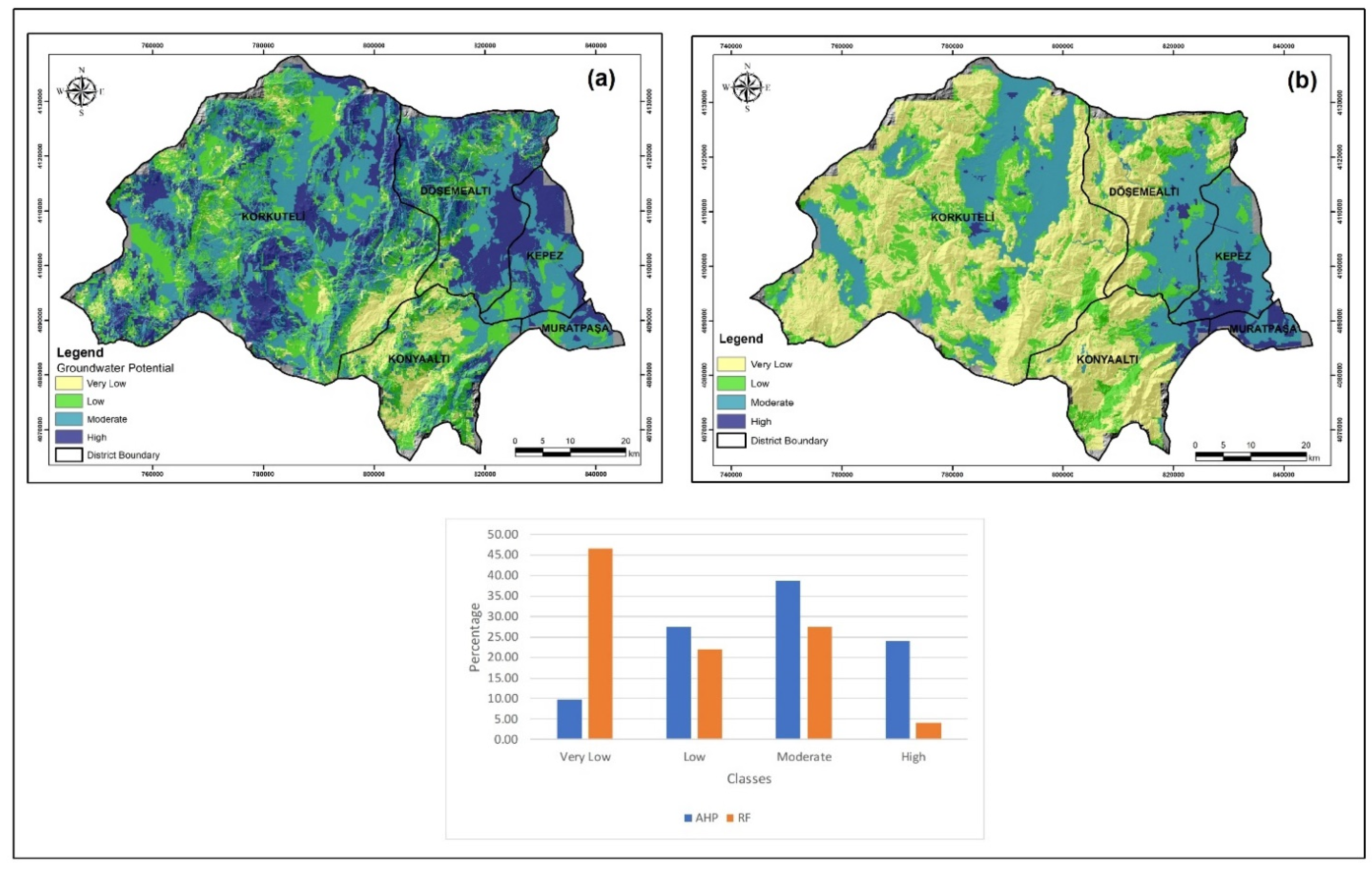
4. Results and Discussion

Considering the seven most influential thematic layers on the groundwater potential, the map deduced from AHP and FR calculation was prepared and classified into four classes based on the Jenk classification scheme in ArcGIS 10.5, ranging from very low, low, and moderate to high classes.
For AHP analysis, a common multicriteria decision-maker model for various geospatial investigations, all the considered thematic layers were classified differently, while most of them were classified into five classes. The factors and sub-classes were weighted and ranked based on their importance and opinions of relevant experts. The overall CR obtained was 0.034, which shows the high consistency of model application. The resultant map by the AHP model (Figure 4a) shows that 24% and 39% of the total area of the central Antalya province is characterized by a moderate and a high groundwater potential (Table 5). These areas have an almost regular distribution over all the districts except for Konyalti. The land coverage shows that areas covered by travertine, alluvium, and agricultural sites have a moderate and a high groundwater potential.
The very low and low potentials are seen over areas covered by less greening or igneous rocks. The frequency ratio (FR) was applied to find the ratio between the percentage of well availability within a certain class and the area of each sub-class of a factor [15]. As described in Table 4, a higher FR is found for sand sediments in which the lithology factor is 9.783.
In the slope factor, flat areas are followed by about 79% of all wells. Hence, the slope less than 16 degrees has the highest FR, which is (1.93). In this study, the frequency ratio becomes high by increasing the drainage density as a density of more than 1.53 km-1 accounts for the highest FR of (3.49). The same trending of ratios was seen in other case studies as well by [4,15]. Considering the landcover pattern, many wells are seen within agricultural and urban areas, which show the highest frequency ratios of 1.5 and 5.57. The most significant number of wells are distributed within the lesser density of lineaments; hence, they have the highest FR of 2.46. The regions highlighted by the highest amount of annual precipitation are characterized by the highest frequency ratio (1.5). Almost 50% of groundwater wells were drilled within the regions with a shallow thickness of soil; therefore, they have a higher FR (1.15). The final resultant map by the FR model was also classified into four classes according to the Jenk classification scheme, showing that 48% of the study area is characterized by a low and a moderate groundwater potential. In contrast, only 4% of the region contains a high potential (Figure 4b) (Table 5).

Validation

Each model must be validated as [43] asserts that a model finds its significance when validated. There are several methods for checking the accuracy and validation of groundwater potential maps generated by AHP and FR models. The most usable validation techniques are receiver operating characteristic (ROC) analysis and area under the curve (AUC), which have been examined by several scholars [4,6,15,20,44]. In this study, wells with high yield and a generated groundwater potential dataset were considered to analyze the ROC curve. The ROC curve was prepared by considering the percentage of groundwater potential classes on the x-axis and the percentage of groundwater wells on the y-axis.
Once the ROC was created, the AUC was calculated to find the accuracy of models and the correct occurrence or non-occurrence of pre-defined classes (Figure 5). The quantitative–qualitative AUC for the AHP model was calculated as 0.56 (or an accuracy of 56%), while the AUC for the FR model resulted in being 0.65 (accuracy of 65%). Based on [15,45], the AUC values corresponding to the prediction accuracy can be divided into poor (0.5–0.6), average (0.6–0.7), good (0.7–0.8), very good (0.8, 0.9), and excellent (0.9–1). Calculation and plotting of the AUC for both models show that the FR model results are more efficient than the AHP model in the study area.

5. Conclusions

Groundwater potential mapping has been carried out using different traditional and remotely based approaches for decades. Remote sensing technology and GIS make it easy and accessible for experts to conduct potential mapping with low effective costs and time consumed. Various spatial and non-spatial modeling techniques using the GIS environment are applied to restrict groundwater potential in which their accuracy is different. In this study, analytical hierarchy and frequency ratio models were applied by considering seven thematic layers: lithology, slope, drainage density, landcover/land use, lineament density, rainfall, and soil depth.
By giving high importance to the lithology of the region and less importance to the soil depth layer, Muratpasa, Kepez, and eastern Dosemealti districts are followed by the high potential of groundwater based on both models. The main reason for the high potential of these districts is the existence of a large travertine plateau which provides an environment for a higher permeability of groundwater. Steep slopes characterize the regions. Additionally, igneous rock coverage is directed to a low and a very low groundwater potential due to huge amounts of runoff on the surface. The areas covered by agricultural and forest areas and alluvium have a moderate potential for groundwater.
The reliability of the AHP model for groundwater potential demarcation is directly dependent on the assignment of the weights and ranks to each class and sub-class. Therefore, deep study and knowledge on factors influencing the targeted object are required. Additionally, the geographical, geological, and hydrological characteristics of the study area are another point to be contemplated. Implementation of the FR does not require more knowledge of users to set ranks or weights, while the model itself finds a ratio of factors that gives more reliable results. The final resultant maps and validation confirm that the groundwater potential mapped by the FR is more efficient and dependable than the AHP model. The results from this study can be a hint for the responsible departments to conduct accurate future planning of groundwater in terms of distribution, planning, consumption, and artificial recharge. Moreover, the findings should be followed with further detailed fieldwork and other relevant studies to accomplish accurate groundwater potential mapping at a large scale over small districts and villages.

Author Contributions

Conceptualization, H.A. and E.P.; methodology, H.A., O.A.K., and E.B.; software, H.A. and O.A.K.; validation, H.A., O.A.K. and E.P.; formal analysis, E.P.; investigation, H.A.; resources, T.S.; data curation, E.B.; writing—original draft preparation, H.A.; writing—review and editing, E.P.; visualization, T.S.; supervision, E.P.; project administration, H.A.; funding acquisition, O.A.K. All authors have read and agreed to the published version of the manuscript.

Funding

This research received no external funding.

Institutional Review Board Statement

Not applicable.

Informed Consent Statement

Not applicable.

Conflicts of Interest

The authors declare that there is no potential conflict arising out of this paper. The paper is also not accompanied by any funding resources.

References

  1. Fitts, C. Groundwater Science; Elsevier: Amsterdam, The Netherlands, 2002. [Google Scholar]
  2. Bagyaraj, M.; Ramkumar, T.; Venkatramanan, S.; Gurugnanam, B. Application of remote sensing and GIS analysis for identifying groundwater potential zone in parts of Kodaikanal Taluk, South India. Front. Earth Sci. 2013, 7, 65–75. [Google Scholar] [CrossRef]
  3. Naghibi, S.A.; Pourghasemi, H.R.; Pourtaghi, Z.S.; Rezaei, A. Groundwater qanat potential mapping using frequency ratio and Shannon’s entropy models in the Moghan watershed, Iran. Earth Sci. Inform. 2015, 8, 171–186. [Google Scholar] [CrossRef]
  4. Das, S. Comparison among influencing factor, frequency ratio, and analytical hierarchy process techniques for groundwater potential zonation in Vaitarna basin, Maharashtra, India. Groundw. Sustain. Dev. 2019, 8, 617–629. [Google Scholar] [CrossRef]
  5. Todd, D.; Mays, L. Groundwater Hydrology; John Wiley & Sons: Hoboken, NJ, USA, 2004. [Google Scholar]
  6. Manap, M.A.; Sulaiman, W.N.A.; Ramli, M.F.; Pradhan, B.; Surip, N. A knowledge-driven GIS modeling technique for groundwater potential mapping at the Upper Langat Basin, Malaysia. Arab. J. Geosci. 2013, 6, 1621–1637. [Google Scholar] [CrossRef]
  7. Senanayake, I.P.; Dissanayake, D.M.D.O.K.; Mayadunna, B.B.; Weerasekera, W.L. An approach to delineate groundwater recharge potential sites in Ambalantota, Sri Lanka using GIS techniques. Geosci. Front. 2016, 7, 115–124. [Google Scholar] [CrossRef]
  8. Banks, D.; Robins, N. An Introduction to Groundwater in Crystalline Bedrock; Norges geologiske undersøkelse: Trondheim, Norway, 2002. [Google Scholar]
  9. Mukherjee, S. Targeting saline aquifer by remote sensing and geophysical methods in a part of Hamirpur-Kanpur, India. Hydrogeol. J. 1996, 19, 53–64. [Google Scholar]
  10. Ganapuram, S.; Kumar, G.T.V.; Krishna, I.V.M.; Kahya, E.; Demirel, M.C. Mapping of groundwater potential zones in the Musi basin using remote sensing data and GIS. Adv. Eng. Softw. 2009, 40, 506–518. [Google Scholar] [CrossRef]
  11. Oh, H.J.; Kim, Y.S.; Choi, J.K.; Park, E.; Lee, S. GIS mapping of regional probabilistic groundwater potential in the area of Pohang City, Korea. J. Hydrol. 2011, 399, 158–172. [Google Scholar] [CrossRef]
  12. Das, S.; Pardeshi, S.D. Integration of different influencing factors in GIS to delineate groundwater potential areas using IF and FR techniques: A study of Pravara basin, Maharashtra, India. Appl. Water Sci. 2018, 8, 197. [Google Scholar] [CrossRef]
  13. Jha, M.K.; Chowdary, V.M.; Chowdhury, A. Groundwater assessment in Salboni Block, West Bengal (India) using remote sensing, geographical information system and multi-criteria decision analysis techniques. Hydrogeol. J. 2010, 18, 1713–1728. [Google Scholar] [CrossRef]
  14. Nampak, H.; Pradhan, B.; Manap, M.A. Application of GIS based data driven evidential belief function model to predict groundwater potential zonation. J. Hydrol. 2014, 513, 283–300. [Google Scholar] [CrossRef]
  15. Razandi, Y.; Pourghasemi, H.R.; Neisani, N.S.; Rahmati, O. Application of analytical hierarchy process, frequency ratio, and certainty factor models for groundwater potential mapping using GIS. Earth Sci. Inform. 2015, 8, 867–883. [Google Scholar] [CrossRef]
  16. Al-Shabeeb, A.A.R.; Al-Adamat, R.; Al-Fugara, H.; AlAyyash, S. Delineating groundwater potential zones within the Azraq Basin of Central Jordan using multi-criteria GIS analysis. Groundw. Sustain. Dev. 2018, 7, 82–90. [Google Scholar] [CrossRef]
  17. Jasrotia, A.S.; Kumar, R.; Saraf, A.K. Delineation of groundwater recharge sites using integrated remote sensing and GIS in Jammu district, India. Int. J. Remote Sens. 2007, 28, 5019–5036. [Google Scholar] [CrossRef]
  18. Magesh, N.S.; Chandrasekar, N.; Soundranayagam, J.P. Delineation of groundwater potential zones in Theni district, Tamil Nadu, using remote sensing, GIS and MIF techniques. Geosci. Front. 2012, 3, 189–196. [Google Scholar] [CrossRef]
  19. Naghibi, S.A.; Moradi Dashtpagerdi, M. Evaluation of four supervised learning methods for groundwater spring potential mapping in Khalkhal region (Iran) using GIS-based features. Hydrogeol. J. 2017, 25, 169–189. [Google Scholar] [CrossRef]
  20. Ozdemir, A. GIS-based groundwater spring potential mapping in the Sultan Mountains (Konya, Turkey) using frequency ratio, weights of evidence and logistic regression methods and their comparison. J. Hydrol. 2011, 411, 290–308. [Google Scholar] [CrossRef]
  21. Sener, E.; Davraz, A. Assessment of groundwater vulnerability based on a modified DRASTIC model, GIS and an analytic hierarchy process (AHP) method: The case of Egirdir Lake basin (Isparta, Turkey). Hydrogeol. J. 2013, 21, 701–714. [Google Scholar] [CrossRef]
  22. Rahmati, O.; Nazari Samani, A.; Mahdavi, M.; Pourghasemi, H.R.; Zeinivand, H. Groundwater potential mapping at Kurdistan region of Iran using analytic hierarchy process and GIS. Arab. J. Geosci. 2015, 8, 7059–7071. [Google Scholar] [CrossRef]
  23. Hossein, A.; Ardakani, H.; Ekhtesasi, M.R. Groundwater potentiality through Analytic Hierarchy Process (AHP) using remote sensing and Geographic Information System (GIS). J. Geope 2016, 6, 75–88. [Google Scholar]
  24. Jenifer, M.A.; Jha, M.K. Comparison of Analytic Hierarchy Process, Catastrophe and Entropy techniques for evaluating groundwater prospect of hard-rock aquifer systems. J. Hydrol. 2017, 548, 605–624. [Google Scholar] [CrossRef]
  25. Guru, B.; Seshan, K.; Bera, S. Frequency ratio model for groundwater potential mapping and its sustainable management in cold desert, India. J. King Saud. Univ.-Sci. 2017, 29, 333–347. [Google Scholar] [CrossRef]
  26. Şener, E.; Şener, Ş.; Davraz, A. Groundwater potential mapping by combining fuzzy-analytic hierarchy process and GIS in Beyşehir Lake Basin, Turkey. Arab. J. Geosci. 2018, 11, 187. [Google Scholar] [CrossRef]
  27. Mogaji, K.A.; Lim, H.S.; Abdullah, K. Regional prediction of groundwater potential mapping in a multifaceted geology terrain using GIS-based Dempster–Shafer model. Arab. J. Geosci. 2015, 8, 3235–3258. [Google Scholar] [CrossRef]
  28. Naghibi, S.A.; Pourghasemi, H.R.; Dixon, B. GIS-based groundwater potential mapping using boosted regression tree, classification and regression tree, and random forest machine learning models in Iran. Environ. Monit. Assess. 2016, 188, 44. [Google Scholar] [CrossRef] [PubMed]
  29. Zabihi, M.; Pourghasemi, H.R.; Pourtaghi, Z.S.; Behzadfar, M. GIS-based multivariate adaptive regression spline and random forest models for groundwater potential mapping in Iran. Environ. Earth Sci. 2016, 75, 665. [Google Scholar] [CrossRef]
  30. Chen, W.; Li, H.; Hou, E.; Wang, S.; Wang, G.; Panahi, M.; Li, T.; Peng, T.; Guo, C.; Niu, C.; et al. GIS-based groundwater potential analysis using novel ensemble weights-of-evidence with logistic regression and functional tree models. Sci. Total Environ. 2018, 634, 853–867. [Google Scholar] [CrossRef]
  31. Lee, S.; Hong, S.M.; Jung, H.S. GIS-based groundwater potential mapping using artificial neural network and support vector machine models: The case of Boryeong city in Korea. Geocarto. Int. 2018, 33, 847–861. [Google Scholar] [CrossRef]
  32. Golkarian, A.; Rahmati, O. Use of a maximum entropy model to identify the key factors that influence groundwater availability on the Gonabad Plain, Iran. Environ. Earth Sci. 2018, 77, 369. [Google Scholar] [CrossRef]
  33. Prasad, R.K.; Mondal, N.C.; Banerjee, P.; Nandakumar, M.V.; Singh, V.S. Deciphering potential groundwater zone in hard rock through the application of GIS. Environ. Geol. 2008, 55, 467–475. [Google Scholar] [CrossRef]
  34. Dinesh Kumar, P.K.; Gopinath, G.; Seralathan, P. International Journal of Remote Sensing Application of remote sensing and GIS for the demarcation of groundwater potential zones of a river basin in Kerala, southwest coast of India Application of remote sensing and GIS for the demarcation of groundwater. Int. J. Remote Sens. 2007, 28, 5583–5601. [Google Scholar] [CrossRef]
  35. Saha, D.; Dhar, Y.; Vittala, S.S. Delineation of groundwater development potential zones in parts of marginal Ganga Alluvial Plain in South Bihar, Eastern India. Environ. Monit. Assess. 2010, 165, 179–191. [Google Scholar] [CrossRef] [PubMed]
  36. Adiat, K.A.N.; Nawawi, M.N.M.; Abdullah, K. Assessing the accuracy of GIS-based elementary multi criteria decision analysis as a spatial prediction tool—A case of predicting potential zones of sustainable groundwater resources. J. Hydrol. 2012, 440–441, 75–89. [Google Scholar] [CrossRef]
  37. Saaty, T. Decision Making for Leaders: The Analytic Hierarchy Process for Decisions in a Complex World; RWS Publications: Pittsburgh, PA, USA, 1990. [Google Scholar]
  38. Kumar, A.; Krishna, A.P. Assessment of groundwater potential zones in coal mining impacted hard-rock terrain of India by integrating geospatial and analytic hierarchy process (AHP) approach. Geocarto. Int. 2018, 33, 105–129. [Google Scholar] [CrossRef]
  39. Hosseinali, F.; Alesheikh, A.A. Weighting spatial information in GIS for copper mining exploration. Am. J. Appl. Sci. 2008, 5, 1187–1198. [Google Scholar] [CrossRef]
  40. Malczewski, J. GIS and Multicriteria Decision Analysis; John Wiley & Sons: Hoboken, NJ, USA, 1999. [Google Scholar]
  41. Saaty, T.L. A scaling method for priorities in hierarchical structures. J. Math Psychol. 1977, 15, 234–281. [Google Scholar] [CrossRef]
  42. Bonham-Carter, F.G. Geographic information systems for geoscientists: Modelling with GIS. Comput. Methods Geosci. 1994, 13, 398. [Google Scholar] [CrossRef]
  43. Fabbri, A.; Chung, C.-J.F.; Fabbri, A.G. Validation of Spatial Prediction Models for Landslide Hazard Mapping. Nat. Hazards 2003, 30, 451–472. [Google Scholar] [CrossRef]
  44. Andualem, T.G.; Demeke, G.G. Groundwater potential assessment using GIS and remote sensing: A case study of Guna tana landscape, upper blue Nile Basin, Ethiopia. J. Hydrol. Reg. Stud. 2019, 24, 100610. [Google Scholar] [CrossRef]
  45. Yesilnacar, E. The Application of Computational Intelligence to Landslide Susceptibility Mapping in Turkey. Ph.D. Thesis, University of Melbourne, Melbourne, Australia, 2005. [Google Scholar]
Figure 1. Location of the study area.
Environsciproc 05 00011 g001
Figure 2. Flowchart describing the methodology.
Environsciproc 05 00011 g002
Figure 3. Thematic spatial maps of study area: (A) lithology, (B) slope, (C) drainage density, (D) landcover/land use, (E) lineament density, (F) rainfall, and (G) soil depth.
Environsciproc 05 00011 g003
Figure 4. The groundwater potential maps for central Antalya, Turkey, by (a) AHP model, and (b) FR model.
Environsciproc 05 00011 g004
Figure 5. Chart showing the ROC curve and AUC for AHP and FR models.
Environsciproc 05 00011 g005
Table 1. Pairwise comparison matrix between all factors for AHP model.
FactorsFactors
LithologySlopeDrainage DensityLandcover/Land UseLineament DensityRainfallSoil Depth
Lithology1.003.004.005.005.007.006.00
Slope1/31.002.002.004.005.006.00
Drainage density1/4½1.002.003.004.005.00
Landcover/land use1/5½1/21.002.003.004.00
Lineament density1/5¼1/31/21.002.003.00
Rainfall1/71/51/41/31/21.001.00
Soil depth1/61/61/51/41/31.001.00
Sum2.295.618.2811.0815.8323.0026.00
Table 2. Normalized pairwise comparison matrix and weights of each factor.
FactorsFactors
LithologySlopeDrainage DensityLandcover/Land UseLineament DensityRainfall Soil DepthWeights
Lithology0.43610.53410.48290.45110.31580.30430.23080.3936
Slope0.14540.17800.24140.18050.25260.21740.23080.2066
Drainage density0.10900.08900.12070.18050.18950.17390.19230.1507
Landcover/land use0.08720.08900.06040.09020.12630.13040.15380.1054
Lineament density0.08720.04450.04020.04510.06320.08700.11540.0689
Rainfall 0.06230.03560.03020.03010.03160.04350.03850.0388
Soil depth0.07270.02970.02410.02260.02110.04350.03850.0360
Sum1.00001.00001.00001.00001.00001.00001.00001.0000
Table 3. Assigned normalized weights and rates for all factors and sub-classes.
NoFactorsSub-ClassesRatingNormalized RatesWeights
1LithologyAlluvium60.1130.3936
Dolomite30.057
Claystone10.019
Limestone70.132
Sand40.075
Melange20.038
Olistostrome 20.038
Travertine60.113
Talus20.038
Sandstone40.075
Pebble30.057
Chert60.113
Shale10.019
Spilitic Basalt20.038
Peridotite20.038
Volkanoclastics20.038
2Slope<16.0750.3330.2066
16.08–32.1440.267
32.15–48.2230.200
48.23–64.2920.133
>64.310.067
3Drainage Density<0.39450.333
0.395–0.72140.2670.1507
0.722–1.0730.200
1.08–1.5220.133
>1.5310.067
4Landcover/Land UseBare Rocks20.0500.1054
Mine Extraction Areas30.075
Natural Grasslands40.100
Forests70.175
Sparse Plants50.125
Waterbodies80.200
Agricultural Areas50.125
Bare Soil40.100
Urban Areas20.050
5Lineament Density<0.2810.0670.0689
0.29–0.5220.133
0.53–0.7530.200
0.76–1.140.267
>1.150.333
6Rainfall <430.9310.0670.0388
430.94–460.4520.133
460.46–489.9730.200
489.98–519.4840.267
>519.4950.333
7Soil DepthShallow20.2000.0360
Moderate30.300
Deep50.500
Table 4. The spatial relationship between factors and wells with an assigned FR for each sub-class.
NoFactorsSub-ClassesNo of PixelsPercentage of Sub-ClassNo of WellsPercentage of WellsFR
1LithologyAlluvium345,07621.256948.942.303
Dolomite10280.0600.000.000
Claystone27370.1700.000.000
Limestone592,05236.46128.510.233
Sand35320.2232.139.783
Melange49,5103.0500.000.000
Olistostrome 16,5881.0200.000.000
Travertine211,01312.994834.042.620
Talus45,6552.8110.710.252
Sandstone220,92113.6074.960.365
Pebble11,1760.6900.000.000
Chert52,3943.2310.710.220
Shale2340.0100.000.000
Spilitic Basalt93090.5700.000.000
Peridotite15,0590.9300.000.000
Volkanoclastics47,7142.9400.000.000
2Slope<16.07662,53240.8011178.721.930
16.08–32.14391,24724.091611.350.471
32.15–48.22319,28619.6642.840.144
48.23–64.29197,24312.1574.960.409
>64.353,5713.3032.130.645
3Drainage Density<0.394401,88924.841712.060.485
0.395–0.721483,39129.872517.730.593
0.722–1.07394,55124.383323.400.960
1.08–1.52256,02715.824129.081.838
>1.5382,2065.082517.733.490
4Landcover/Land UseBare Rocks35,4182.1800.000.000
Mine Extraction Areas93760.5800.000.000
Natural Grasslands82,1595.0685.671.121
Forests668,03741.172920.570.500
Sparse Plants219,73613.5432.130.157
Waterbodies31680.2000.000.000
Agricultural Areas535,47833.007049.651.504
Bare Soil52560.3200.000.000
Urban Areas63,9773.943121.995.576
5Lineament Density<0.2859,63014.715136.172.460
0.29–0.52111,17627.423524.820.905
0.53–0.75123,27430.403726.240.863
0.76–1.183,00120.47107.090.346
>1.128,4167.0185.670.810
6Rainfall <430.9353,9333.2864.261.298
430.94–460.45234,15514.2496.380.448
460.46–489.97674,20240.994632.620.796
489.98–519.48566,16334.426546.101.339
>519.49116,4407.081510.641.503
7Soil DepthShallow717,95644.237251.061.155
Moderate648,62039.964733.330.834
Deep256,65615.812215.600.987
Table 5. The distribution of groundwater potential classes based on AHP and FR models.
ClassAHP ModelFR Model
RangeArea (km2)Area (%)RangeArea (km2)Area (%)
Very Low0.0743–0.1472377.1259.712.4140–5.60051807.73346.54
Low0.1473–0.17171068.5427.515.6006–8.6277853.672521.98
Moderate0.1718–0.19221508.57538.848.6278–12.77021066.23827.45
High0.1923–0.243930.1723.9512.7703–22.7280156.82754.04
Publisher’s Note: MDPI stays neutral with regard to jurisdictional claims in published maps and institutional affiliations.

