Statistical Analysis for Long-Term Weather Forecast ^†

Abstract

A weather forecast is a result of applying science and technology to predict the conditions of the atmosphere in a selected location and time in the future. The main input is a collection of data (atmospheric, land, and ocean), and the resulting output is meteorology (how atmospheric conditions will change). People have been trying to predict the weather by observing nature for thousands of years, but in a scientific way only since the 19th century. First manually and based mostly on changes in barometric pressure, and later in modern times with the contribution of computer-based models (numerical weather prediction). Despite the high inaccuracy of numerical weather prediction beyond 10 days, the interest in long-term weather forecasts is very high due to social reasons—energy sector, civil protection, etc.—and the scientific effort is constant. Here, we propose a statistical weather model for long-term weather forecasts based on weather/climate data time series. We will analyze atmospheric data in 850 hPa for a period of 35 years, resulting in temperature ensembles and temperature deviations for specific periods. Finally, we will contrast the results of the statistical weather model (prediction) with the real data to check the accuracy of the model.

1. Introduction

A long-term weather forecast is the Holy Grail of meteorology. Supercomputers and numerical methods [1] are combined to improve weather forecasts beyond 10 days. Despite the applied high science and technology, results are poor due to fundamental obstacles in numerical forecast [2]. Therefore, long-term weather forecast is produced mostly from models based on statistical analysis.

Statistical analysis is the in-depth study of a problem using calculations, tables, and charts in order to produce statistical conclusions [3]. The presentation of the primary statistical material is called classification [4], with geometrical classification and time series classification as the most important subsets.

Time series classification (TSC) [5] is the tracking of the evolution of a variable over time. Time series are described with one or more of the following features:

A long-term trend.

A periodical trend.

Some irregular or random variations.

Statistical analysis of a time series is recommended to describe the regularity that may exist between successive values of a variable having as a purpose to predict the future behavior of that series.

2. Method

The method is based on a time-series analysis of temperature data at 850 hPa. The layer of 850 hPa is selected because it is not affected by surface conditions like the Foehn effect [6], temperature inversion [7], or urban heat island effect [8].

Ten major administrative regions of Greece (Thrace, Macedonia, Epirus, Thessaly, Ionian islands/West Greece, Central Greece/Attica/Euboea, Peloponnese, North Aegean, Crete, and South Aegean) are selected, representing the grids of the study. For each grid, a dataset of daily temperatures in 850 hPa for the last 35 years is downloaded from the Physicals Science Laboratory, NOAA [9], and registered in a database.

Since the registration is completed, the database is simplified in 5-day periods and interfaced with the formula of the model.

The formula is a machine learning algorithm based on climate and astronomical cycles—El Nino, La Nina, and solar cycles—and statistical weights, sums, and possibilities. It is described by four main processes:

• Calculation of average temperatures in periods of 35, 22, 9, and 7 years (A35, A22, A9, and A7 values) (Figure 1);

2.

Comparison of last period temperatures with A35 values—0 for lower values and 1 for higher values (B values) (Figure 2);

3.

Calculation of average B values in periods of 22, 9, and 7 years (C22, C9, and C7 values—grey) and calculation of corresponding D values (statistical weights) (D22, D9, and D7 values—red) (Figure 3);

4.

Calculation of prediction values based on the formula:

[A35 value] + or − (depending on the D22 value) [ABS of A22 value] + or − (depending on the D9 value) [ABS of A9 value] + or − (depending on the D7 value) [ABS of A22 value]

For each season, the model produces 18 prediction values (6 per month), resulting in a temperature ensemble for each studied region (Figure 4).

Predictions proceed into a second-level analysis resulting in temperature deviations (Figure 5), and they are plotted in weather maps (Figure 6).

The total amount of information (temperature ensembles, temperature deviations, and weather maps) is combined for translating data into text. Short paragraphs are published with reference to possible dates with significant changes in weather circulation.

3. Results

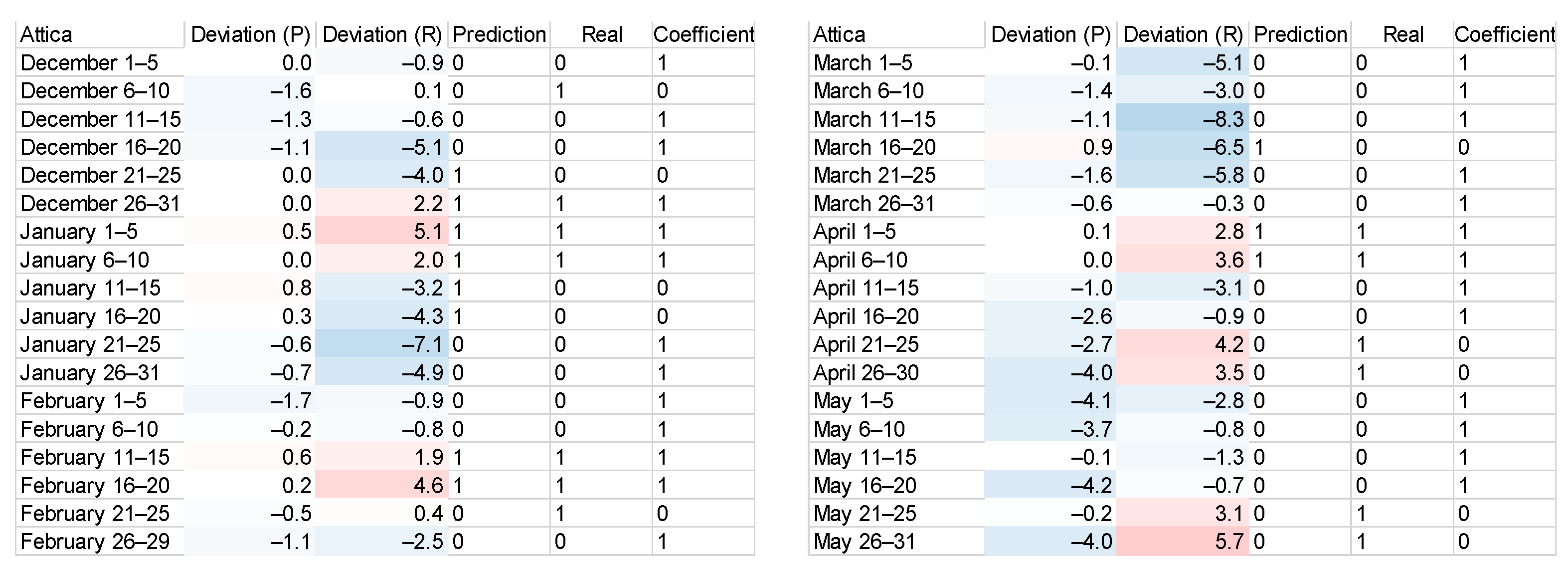
We will examine the accuracy of the model for the period 1 December 2021 till 30 November 2022 in terms of deviation trend, separated into four (4) seasons and with respect to the grid of Attica.

We start with the registration of the predicted deviation values and real deviation values downloaded from the Physicals Science Laboratory, NOAA [9]. Since we built the dataset, we proceeded to the transformation of values—1 for positive values and 0 for negative values. Identical values result in 1, and non-identical values in 0 (Figure 7).

According to the resulting coefficient, the accuracy of each season is the following:

• Winter: 72.2%;
• Spring: 72.2%;
• Summer: 38.9%;
• Autumn: 61.1%.

We observe that winter, spring, and summer meet medium to high scores, while summer meets low scores. Analyzing the accuracy of each month, we have the following results:

• December: 66.7%;
• January: 66.7%;
• February: 83.3%;
• March: 83.3%;
• April: 66.7%;
• May: 66.7%;
• June: 16.7%;
• July: 50%;
• August: 50%;
• September: 66.7%;
• October: 100%;
• November: 16.7%.

Among twelve months, three months meet high scores (February, March, October), five months meet higher-than-average scores (December, January, April, May, September), two months meet average scores (July and August), and two months meet low scores (June and November).

The above results show a weakness in algorithmic function during the summer period, as well as for November. In contrast, from December to May (as well as September), the results show a strong algorithmic functionality, while October meets an exceptional score.

The dysfunctionality of the summer period is under investigation. A mismatch in the order of D and A values in the formula has been detected, it is corrected, and it will be reevaluated in the next seasonal prediction (published on 19 May 2023) [11].

Further research is required, involving more seasons/years of predictions to detect specific dysfunctionalities of the algorithm and to confirm the good results as well. Additionally, the method should be applied in more grids, and globally if possible, to ensure total application (ongoing). A final and more complicated step is the application of the method with temperature data in 500 hPa and the combination of resulting values in 850 hPa and 500 hPa for a more accurate prediction.

References

- Numerical Weather Prediction (Weather Models). Available online: https://www.weather.gov/media/ajk/brochures/NumericalWeatherPrediction.pdf (accessed on 12 April 2023).
- Mailier, P. Can We Trust Long-Range Weather Forecasts? In Management of Weather and Climate Risk in the Energy Industry; Springer: Berlin/Heidelberg, Germany, 2010; pp. 227–239. [Google Scholar]
- Ali, Z.; Bhaskar, S.B. Basic statistical tools in research and data analysis. Indian J. Anaesth. 2016, 60, 662–669. [Google Scholar] [CrossRef] [PubMed]
- Data classification analysis. Available online: https://www.ibm.com/docs/en/iis/11.7?topic=dcao-data-classification-analysis (accessed on 13 April 2023).
- Fawaz, H.; Forestier, G.; Weber, J.; Idoumghar, L.; Muller, P. Deep learning for time series classification: A review. Data Min. Knowl. Discov. 2019, 33, 917–963. [Google Scholar] [CrossRef]
- Foehn Effect. Available online: https://www.metoffice.gov.uk/weather/learn-about/weather/types-of-weather/wind/foehn-effect (accessed on 22 April 2023).
- What Is a Temperature Inversion? Available online: https://www.metoffice.gov.uk/weather/learn-about/weather/types-of-weather/temperature/temperature-inversion (accessed on 22 April 2023).
- Urban Climate Impacts. Available online: https://www.metoffice.gov.uk/research/climate/climate-impacts/urban (accessed on 22 April 2023).
- Physical Science Laboratory. Available online: https://psl.noaa.gov/data/gridded/data.ncep.reanalysis.html (accessed on 28 May 2023).
- YouWeather Statistical Model (YSM)—Άνοιξη 2022 (Ελλάδα). Available online: https://www.youweather.com/el-gr/article/o-kairos-tin-anoixi-2022-stin-ellada.html (accessed on 5 May 2023).
- YouWeather. Available online: https://www.youweather.com/el-gr/article/ysm-o-kairos-to-kalokairi-2023-stin-ellada.html (accessed on 5 May 2023).
Figure 1.
Average temperatures in 850 hPa.
Figure 2.
B values (deviation to 35 years’ average temperature).
Figure 3.
C values and D values.
Figure 4.
Temperature ensembles for a predicted period [10].
Figure 5.
Deviation table. Gradient color scale from −30 degrees Celsius (negative deviation: deep blue to light blue) to +30 degrees Celcius (positive deviation: light red to deep red) [10].
Figure 6.
Plotting of deviation (5-day periods). Gradient color scale from −30 degrees Celsius (negative deviation: deep blue to light blue) to +30 degrees Celcius (positive deviation: light red to deep red) [10].
Figure 7.
Predicted deviation vs. real deviation and coefficient values (per season). Gradient color scale from -30 degrees Celsius (negative deviation: deep blue to light blue) to +30 degrees Celcius (positive deviation: light red to deep red).
Disclaimer/Publisher’s Note: The statements, opinions and data contained in all publications are solely those of the individual author(s) and contributor(s) and not of MDPI and/or the editor(s). MDPI and/or the editor(s) disclaim responsibility for any injury to people or property resulting from any ideas, methods, instructions or products referred to in the content. |
© 2023 by the author. Licensee MDPI, Basel, Switzerland. This article is an open access article distributed under the terms and conditions of the Creative Commons Attribution (CC BY) license (https://creativecommons.org/licenses/by/4.0/).
Share and Cite
MDPI and ACS Style
Kampolis, D. Statistical Analysis for Long-Term Weather Forecast. Environ. Sci. Proc. 2023, 26, 30. https://doi.org/10.3390/environsciproc2023026030
AMA Style
Kampolis D. Statistical Analysis for Long-Term Weather Forecast. Environmental Sciences Proceedings. 2023; 26(1):30. https://doi.org/10.3390/environsciproc2023026030
Chicago/Turabian StyleKampolis, Dimitrios. 2023. "Statistical Analysis for Long-Term Weather Forecast" Environmental Sciences Proceedings 26, no. 1: 30. https://doi.org/10.3390/environsciproc2023026030